1. Introduction
Beginning with the launch of N07 in June 1981, two generations of the Advanced Very High-Resolution Radiometers, AVHRR/2s and 3s (see Abbreviations), have been flown onboard ten NOAA satellites, N07, N09, N11, N12, N14, N16, N17, N18, and N19 ([
1] and references therein). The AVHRRs measure top-of-the-atmosphere brightness temperatures (BTs) in three thermal infrared (IR) bands, centered at 3.7 µm (band 3 on AVHRR/2; 3b on AVHRR/3), 10.8 µm (band 4) and 12 µm (band 5), along with two reflectances in bands 1 (0.63 µm) and 2 (0.83 µm). Original AVHRR measurements with a spatial resolution of 1.1 km at nadir (degrading to ~7 km at the edges of the ~3000 km swath) are sub-sampled onboard NOAA satellites to ~4 km resolution at nadir (~25 km at swath edge) and transmitted to the ground, comprising the widely known Global Area Coverage (GAC) format. The NOAA GAC observations from AVHRR/2s and/3s enable the creation of multi-year, multi-satellite global datasets of sea surface temperature (SST) [
2,
3,
4,
5,
6], one of the essential climate variables according to the World Meteorological Organization [
7].
Altogether, the NOAA satellites comprise the US first-generation Low Earth Orbiting (LEO) constellation (aka the Polar Operational Environmental Satellites, POES). As of this writing, AVHRRs onboard seven of them are dead, while the remaining three (N15, N18, and N19) continue providing L1b data, which are of some (although limited, due to their age and degraded functionality) use for SST retrievals. These remaining POES satellites are designated as backups for the US second-generation operational LEO constellation, the Joint Polar Satellite System (JPSS). The first satellite in the JPSS series, the Suomi National Polar-orbiting Partnership (NPP) satellite, was launched in Oct 2011, and N20 followed in Nov 2017. Both carry the Visible Infrared Imager Radiometer Suite (VIIRS), with much improved SST capabilities over the AVHRR, and fly half-orbit away from each other. Three more JPSS satellites are in the queue: J2/N21 (scheduled for launch in Nov 2022), J3/N22 (2026), and J4/N23 (2031). With a 7-year nominal design life and based on the NPP 10+ year stable performance so far, the JPSS series is expected to continue into the 2040s, resulting in a ~30 yrs JPSS SST record, of which ~10 years are currently available [
8]. The 40+ years of POES and ~30 years of JPSS are expected to result in a 60+ years SST record, with a ~10+ years overlap. In conjunction with the 20+ years of MODIS data onboard Terra and Aqua, 15+ years of AVHRR FRAC onboard European Metop First Generation [
9], and METImage onboard the future Metop Second Generation series, the NOAA POES and JPSS SST data form a solid foundation for a consistent long-term LEO SST record. It is critically important to process data from different platforms and sensors with maximal consistency. The NOAA enterprise SST system, Advanced Clear Sky Processor for Ocean (ACSPO) [
10,
11,
12], was designed to process the entire LEO (as well as geostationary) data records and is well-positioned to create long-term, consistent SST time series.
In this context, the AVHRR GAC SST Reanalysis 2 (RAN2) dataset has been created at NOAA and documented in this paper. The RAN2 builds upon the RAN1 released in 2016, which covered a period from 2002–2016, and improves its temporal coverage (Sep 1981–Dec 2021) and overall data completeness and quality. The cross-satellite consistency and stability of SSTs are achieved by fitting each satellite SST to in situ SST, within an optimal retrieval domain. RAN2 mitigates a number of the NOAA orbital and AVHRR instrumental issues, as well as addresses the lack of, and/or poor quality of the auxiliary information, particularly during the early AVHRR period in the 1980−90s [
13,
14,
15]. In [
16], the performance of an interim version of RAN2 (RAN2 Beta 01, produced at the initial stage of the RAN2 project and available for a limited period from 1981–2003) was preliminarily compared with two other available long-term reprocessed AVHRR GAC SST datasets: the NOAA Pathfinder v5.3 (PF) [
3,
4] and the ESA Climate Change Initiative v2.1 (CCI) [
5,
6]. In this paper, the RAN2 SST is consistently validated against quality-controlled in situ data from the NOAA in situ Quality Monitor (
iQuam, [
17,
18,
19,
20]). Additionally, the comparisons with PF and CCI are expanded to the full period covered by the released RAN2 dataset, from Sep 1981–Dec 2021, using the NOAA SST Quality Monitor (SQUAM, [
21,
22]) system.
2. RAN2 Dataset
2.1. Handling AVHRR Data
Table 1 lists the NOAA satellites processed in RAN2, including the abbreviations of satellites’ names used in the paper, the AVHRR instruments, types of orbits, and the local equator crossing times (LEXTs) at the beginning of each mission, and periods of data processed in RAN2. As of this writing, the full RAN2 SST dataset covers a period from 1 Sep 1981–31 Dec 2021. Full historical L1b data were obtained from the NOAA Center for Satellite Application and Research (STAR) Central Data Repository (SCDR) system. The RAN2 SSTs are produced from three AVHRR thermal IR bands centered at 3.7 µm (band 3 in AVHRR/2, 3b in AVHRR/3), 10.8 µm (band 4), and 12 µm (band 5) at night, and from bands 4 and 5 during the daytime, in a full swath, VZA < ±68°. The algorithms are switched over at the solar zenith angle, SZA = 90° (defined in the pixel at the Earth’s surface).
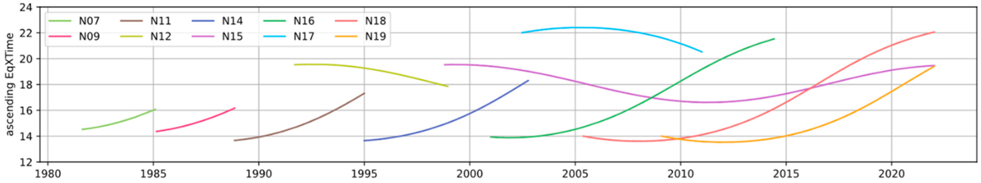
The orbits of the NOAA satellites are not corrected in flight, which results in significant evolutions of the LEXT during each mission, as shown in
Figure 1 taken from the NOAA Sensor Stability for SST system, 3S [
23,
24]. As a result, the NOAA AVHRRs observe the ocean surface at different phases of the diurnal cycle and under variable thermal regimes of the sensors. The orbital drift, along with the aging of the AVHRR optical sub-systems and detectors, causes long-term trends in the AVHRR brightness temperatures (BTs), which are not fully accounted for in the calibration coefficients available in the NOAA operational L1b data (which have not been reprocessed, as of this writing). In the NOAA AVHRR Reanalyses (RANs) [
2,
9,
13,
14,
15,
16], long-term BT trends are mitigated by retraining SST regression coefficients on a daily basis.
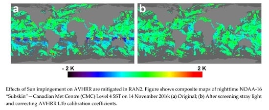
When the satellite flies near the terminator, its AVHRR sensor is exposed to sunlight [
23,
25,
26]. When approaching the terminator from the dark side of the orbit, (i.e., coming out of the Earth’s shadow), the Sun impinges on the internal calibration target (ICT, or black body), resulting in incorrect and often erratic calibration coefficients (slope/gain and intercept). Typically, up to ~2000–2500 AVHRR GAC 0.5-sec scans are affected. Using the corrupted calibration coefficients reported in the operational NOAA L1b files results in incorrectly calculated BTs from the sensor counts recorded on L1b, which in turn leads to abnormally cold SST retrievals. On the other hand, the stray light in the Earth view leads to warm outliers in BTs and retrieved SSTs. In RAN2, the corrupted calibration coefficients on the dark side are corrected by interpolation of the L1b gain and offset between the unaffected parts of the orbits, whereas the Earth view pixels contaminated with the stray light are detected by the elevated signal in channel 2 and filtered out [
15].
In addition, some observations from N07, N11, and N12 were affected by three major volcanic eruptions, Mt. El Chichon (Mar 1982), Mt. Pinatubo (Jun 1991), and Mt. Hudson (Aug–Oct 1991). For several months following each eruption, the Earth’s atmosphere was contaminated with volcanic aerosols, leading to massive cold outliers in retrieved SSTs, e.g., [
27,
28]. The modifications to the ACSPO Clear-Sky Mask (ACSM) [
10] were made to filter out BTs and SSTs affected by volcanic aerosols [
14].
2.2. Training RAN2 SST Algorithms against In Situ SSTs
ACSPO employs regression-based SST retrieval algorithms with coefficients derived from matchups of clear-sky satellite BTs with in situ SST,
TIS. The
TIS data are obtained from the NOAA
iQuam system [
18,
19]. Traditionally, the regression coefficients are trained against drifting and tropical moored buoys, (D + TM). However, as shown in
Figure 2, the number of (D + TM) observations in the 1980−90s was critically small. Matching in situ SSTs with clear-sky satellite observations further reduces the number of usable (D + TM) data by ~80–90%, making them insufficient for training purposes. On the other hand, the number of SST measurements from ships during this period far exceeded the number of observations from (D + TM)’s. Despite their relatively low accuracy and precision [
17,
20], including ship data in the training, i.e., using (S + D + TM), was found beneficial for N07 and N09. For all later satellites, N11 to N19, only (D + TM) were used for training. The training matchup data sets (MDS) were accumulated within space/time windows of ±10 km/±2 h for N07 through N15, and within ±10 km/±30 min for N16 through N19. The matchups were collected with the ‘one-to-many’ method, according to which all satellite pixels within the space/time windows are matched up with the central in situ anchor. Each pair in the MDS is considered an independent matchup.
2.3. Auxiliary Data in RAN2
An important component of the ACSPO auxiliary data is ‘first guess’ SST,
T0, obtained by interpolation of analysis L4 SST to sensor’s pixels. The ACSPO employs retrieval algorithms of the NLSST type [
29], in which a high correlation of
T0-dependent regressors with
TIS helps suppress the noise in retrieved SST. The ACSM [
10] also uses the deviation of retrieved SST from
T0 as one of the cloud predictors. Hence, the consistency of
T0 with
TIS is essential for quality SST retrievals. The ACSPO customarily derives
T0 from L4 SST by the Canadian Meteorological Center (CMC) [
30]. In RAN2, the CMC L4 is used for SST retrievals since its first date on 1 September 1991. This includes the second part of the N11 mission and all subsequent missions. For the earlier missions of N07, N09, and the first part of the N11 mission,
T0 was derived from the analysis L4 ‘depth’ SST produced by the European Space Agency Climate Change Initiative v.2.1 (CCI), available from 1 Sep 1981–31 December 2018 [
5,
6].
To illustrate the consistency between
T0’s employed in RAN2 and
TIS from 1981–present,
Figure 3 shows the time series of the monthly mean and standard deviations (SDs) of the Δ
Ts =
TIS −
T0. Mission-averaged means (
µ) and SDs (
σ) are also shown, one set per satellite. (The only exception is N11, for which two sets of
µ and
σ are shown, separately, for the periods before and after 1 Sep 1991, when the ‘first guess’ changed from CCI to CMC. Recall that the training MDSs include matchups with (S + D + TM) for N07/09 and with (D + TM) for later satellites. The Δ
Ts biases are unstable before 1 September 1991, when the CCI L4 SST was used as
T0. The exclusion of ships from the N11 MDS does not reduce the variability of biases prior to 1 September 1991 but makes them on average −0.13 K colder (because ships are overall biased warm with respect to (D + TM) [
17,
30]). When CMC L4 was used (for the second part of N11 and all subsequent missions), the Δ
Ts biases are more stable.
In addition to gradual improvement of the (D + TM) SSTs in time, the long-term trends in the Δ
Ts biases are largely determined by the initial orbital configuration of a particular NOAA satellite, and its evolution in time (cf.
Figure 1). The warmest biases are observed for the satellites in the early morning orbits, which include the full mission of N12, N15 before 2005 and after 2016, N18 after 2017, and N19 after 2020. The biases are coldest for the satellites flying in the afternoon orbits (i.e., full missions of N11/14/16, as well as N18 before 2016 and N19 before 2020). Short-term seasonal variability of the Δ
Ts is caused by the annual evolution of the diurnal thermocline between the
TIS (measured by the D + TM at 0.2–1 m depths) and the
T0 (CMC foundation SST, which is characteristic of the water layer with no diurnal variability). The SDs of Δ
Ts are close to 1 K for N07/09 and drop to 0.5 K in the first part of the N11 mission, due to the exclusion of ship data from the training MDS. In the second part of the N11 mission, the SDs reduce to 0.26 K and remain close to this level for all subsequent satellites.
The first guess SST is also used in ACSPO for simulation of clear-sky BTs with the Community Radiative Transfer Model (CRTM) [
31], using
T0 and vertical profiles of the atmospheric temperature and humidity from the NASA Modern-Era Retrospective Analysis for Research and Applications (MERRA) [
32,
33] as inputs. Simulated BTs are used to monitor the measured BTs for stability and cross-platform consistency and validate CRTM and its inputs (including the
T0 and MERRA profiles).
Future work should include developing a more consistent and stable L4 analysis for use in ACSPO RANs. Efforts should be also taken to reduce ACSPO reliance on the first guess SST and to improve the uniformity and consistency of in situ data used for Cal/Val. For RAN2, however, users should be aware of the limitations discussed above.
2.4. RAN2 Output
As of this writing, the full dataset of RAN2 AVHRR GAC SST is available on the NOAA CoastWatch website
https://coastwatch.noaa.gov/cw/satellite-data-products/sea-surface-temperature/acspo-avhrr-gac.html (accessed on 30 June 2022), in three formats: L2P (swath), L3U (gridded uncollated) and L3C (gridded collated). All products are compliant with the Group for High-Resolution SST (GHRSST) Data Specification v2 (GDS2) standard [
34]. The L2P data are reported in 10-min granules (~5 MB/file), 144 files/24 h, with ~8 TB total data size from 1 September 1981–present. The 0.02° L3U data are produced from L2P and reported in 10-min granules, 144 files/24 h with a ~12 TB total data size. (Note that the L3U GAC data size is larger than L2P because 4 km at nadir to 25 km at swath edge L2P data are uniformly mapped onto a finer 0.02° grid, effectively close to a 2 km global resolution. This is performed intentionally, to ensure consistency with all other ACSPO Level 3 (L3U, L3C, and L3S) products derived from higher-resolution sensors, such as AVHRR FRAC, MODIS, and VIIRS. The 0.02° L3C data are produced by collating various satellite overpasses reported in L3U and saving the product in two files/24 h, separately for day and night, with ~10 TB total data volume. Only data with quality level QL = 5 (classified as ‘clear-sky’ by the ACSM) are recommended for use and evaluated in this study.
3. Other Datasets Used in This Study for Comparison
3.1. Pathfinder v5.3 (PF)
The PF is a 4 km L3C (gridded collated) SST dataset produced by the NOAA National Centers for Environmental Information (NCEI) [
3,
4]. It is reported in two files per 24 h, one for day (SZA < 90°) and one for night (SZA ≳ 90°). The PF SST is produced within a limited range of VZAs, |VZA| < 55°, with regression equations employing two AVHRR bands 4 (10.8) and 5 (12 µm), during both day and night. The regression coefficients are recalculated on a monthly basis, for two atmospheric water vapor regimes: dry and medium-to-moist atmospheres, defined by the BT difference between AVHRR bands 4 and 5. The PF ‘skin’ SST is obtained from the retrieved SST (trained against in situ SST) by subtracting a ‘depth-to-skin’ bias of 0.17 K. To facilitate comparisons of the PF ‘skin’ and RAN2 ‘subskin’ SSTs in this study, the +0.17 K bias was added back. The PF dataset reports SST from one satellite at a time, does not include the early-morning satellites N12 and N15, and does not provide separate estimates of ‘depth’ SST. At the time of this writing, the PF v5.3 covers a period from 25 August 1981–31 December 2021. Per PF developers’ recommendation, data with Q and 5 are used in the comparisons below.
3.2. Climate Change Initiative v2.1 (CCI)
The CCI dataset [
4,
5] reports both ‘skin’ and ‘depth’ SSTs. The ‘skin’ SST is retrieved from two AVHRR bands 4 and 5 during the day, and three bands 3/3b, 4, and 5 at night, with the algorithms switched over at SZA = 92.5°. Retrievals are made using a radiative transfer model-based Optimal Estimation (OE) method [
35]. The ‘depth’ SST is produced from ‘skin’ SST using parameterization of the skin layer and diurnal thermocline, with NWP model surface fluxes and wind stress as inputs [
5]. In contrast with the RAN2 and PF SSTs, produced with regression algorithms trained against in situ SSTs, the OE does not explicitly use in situ data for ‘skin’ SST retrievals, resulting in SST being less dependent on in situ SSTs. A higher degree of independence was achieved after 1995, when AVHRR BTs were anchored to ATSR/2 and AATSR BTs [
5]. Prior to that period, CCI employed in situ SSTs as a ‘calibration’ reference, on large scales. As recommended by data producers, SSTs with QL = 4 and 5 are used in comparisons [
5]. Note that lower QLs are assigned to the retrieved SSTs in some specific VZA and SZA regimes [
36]. For |VZA| > 60°, QL ≤ 2. In the twilight zone (60° < SZA < 92.5°), QL ≤ 3. These conditions are excluded by the QL = 4 and 5 criteria.
The CCI dataset provides SST retrievals from individual satellites in three formats: L2P, L3U, and L3C, which are further aggregated into CCI L4 analysis. The CCI L2P swath data are reported in ~110-min orbital files, 13–14 files/24 h. The L3U (gridded uncollated) data are produced by gridding L2P data with 0.05° resolution, also 13–14 files/24 h. The same 0.05° resolution L3C (gridded collated) data are produced by aggregating all L3U data into two files/24 h, one for the day and one for the night. As of this writing, the AVHRR GAC CCI v2.1 dataset covers a period from 24 Aug 1981–31 Dec 2018. In all analyses below, +0.17 K was added to CCI ‘skin’ SSTs, to facilitate comparisons with RAN2 ‘subskin’ SSTs.
4. Temporal and Spatial Coverage
4.1. Processed Periods
Figure 4 shows periods covered by satellite data. Note that SSTs from N12 and N15 were not processed in PF. Data of N14–N19 are more completely represented in RAN2.
4.2. Global and Regional Imagery
Figure 5 shows global maps of RAN2 ‘subskin’ SSTs, as well as CCI and PF ‘skin’ SSTs + 0.17 K, produced from the corresponding nighttime N18 L3C data for 1 January 2009. Overall, the coverage in both CCI and PF appears more conservative than in RAN2 (even in the areas where all three products report valid SSTs). Recall also that the RAN2 reports QL = 5 data within full scan (VZA < ±68°), whereas the CCI and PF SSTs with QL = 4 and 5 are limited to VZA ranges of < ±60° and < ±55°, respectively, causing inter-orbital swaths with missing data, which are wider in the PF.
Figure 6 shows example regional imagery over the Gulf of Mexico and the Caribbean Sea, from the same N18 satellite and on the same night of 1 January 2009 as in
Figure 5. Overall, the SST patterns are similar in all three products. In the CCI and PF images, the SST is not reported over significant parts of the Caribbean Sea, outside their respective VZA cutoffs. Interestingly, not all CCI grid nodes are filled with valid SSTs (with any QL, including < 4), and the number of such blank pixels increases with VZA. (This effect is also observed in PF, but only at |VZA| > 55° not covered by QL = 4 and 5 and therefore not seen in
Figure 6). Blank grid nodes appear in the CCI and PF L3C products at large VZAs, where the separation between the AVHRR fields of view exceeds the spacing between the neighboring grid nodes. In RAN2, the blank nodes are filled in by the interpolation between the neighboring L2P pixels [
37].
Daytime SST imagery (not shown here) shows similar observations, namely, more complete coverage in RAN2, due to processing full sensor swath, less conservative masking, and filled L3C SST imagery from the ambient L2P pixels.
4.3. Clear-Sky Ratios
This section compares coverage of the world ocean with valid SST data in RAN2, PF, and CCI. The coverage is estimated in terms of monthly Clear-Sky Ratio (CSR) defined as
R =
NCS/NO, where
NCS is a number of identified clear-sky pixels and
NO is a total number of ocean pixels observed during a given month. Note that the CSR metric allows comparisons of the products with different spatial resolutions, i.e., 0.02° in RAN2, 0.05° in CCI, and 4 km in PF. Note also that the calculation of
NO requires land and ice pixels to be excluded from the compared products. Land and ice masks are available in the RAN2 L2P and L3C, PF L3C, and CCI L2P products, but they are not included in the CCI L3C files. Therefore, we separately compared the CSRs in the RAN2 and PF L3C products (
Figure 7), and then in RAN2 and CCI L2P products (
Figure 8). Note that the process of gridding and further collating from L2P to L3U to L3C may increase the CSR [
37].
Figure 7 shows that RAN2 provides from ×2.0–2.7 increased coverage compared with PF (no comparison is possible for the early-morning satellites, N12 and N15, which recall are not included in the PF dataset).
Figure 8 compares CSRs in RAN2 and CCI L2P products. On average, RAN2 provides ×1.8–2.5 higher coverage than CCI for all satellites except the early-morning N12 and N15, for which the margin is wider, ×3.3–5.4. The next section shows that margins between RAN2 and CCI are wider for the N12/15, because the effects of Sun impingement in CCI are not mitigated, and CCI Quality Level is simply reduced in the twilight zone (QL ≤ 3) (and not only at night but also during the daytime, too). The degraded QLs are responsible for significantly reduced CSRs in the CCI dataset for the N12 and N15 missions.
Note also that the comparison of RAN2 L3C coverage in
Figure 7 with the RAN2 L2P in
Figure 8 suggests that the collation increases the CSR by 30–60%, as expected [
37].
4.4. Latitudinal Hovmöller Diagrams of ‘Subskin/Skin’ – (D + TM) SST
This section provides additional insight into the spatial and temporal structure of the retrieved nighttime ‘subskin/skin’ minus (D + TM) SST residuals in the three datasets, with the examples of their corresponding latitudinal Hovmöller diagrams.
Figure 9 shows such diagrams for N11. The most prominent features in
Figure 9 are the cold spots after mid-1991, in all three diagrams. Those are caused by the contaminations of the atmosphere with volcanic aerosols, following eruptions of Mt. Pinatubo and Mt. Hudson in the summer of 1991 [
27]. However, their intensity is different. In RAN2, they are less pronounced than in CCI because the ACSM employed in RAN2 was designed to be more conservative in latitudinal bands with an abnormally large number of cold SST outliers [
14]. In PF, the cold spot in 1991 is more intensive and widespread than in CCI. Recall that the PF uses a two-band SST retrieval algorithm at night, which may be more sensitive to the volcanic aerosol than the three-band nighttime algorithms employed in RAN2 and CCI. Sparser coverage and cold spots, caused by the Sun’s impingement on the ICT, are also noticeable in the CCI and PF SSTs around 1994. In RAN2, the pixels in this area were restored by correcting the L1b thermal calibration, and their SSTs are more realistic [
15].
Overall, the RAN2 Hovmöller diagrams are populated more densely and fully than in CCI and PF, with fewer ‘salt-n-pepper’ features, thus facilitating analyses of the extent and amplitude of the regional biases in RAN2, and their evolution in time.
Figure 10 shows Hovmöller diagrams for nighttime N12 RAN2 ‘subskin’ and CCI ‘skin’ SSTs. Note that the N12 was flying in the early morning orbit, which resulted in frequent Sun impingements on its AVHRR. A comparison of the RAN2 and CCI diagrams reveals the different handling of such events. In CCI, the pixels affected by both the Sun’s impingements on the black body, and by the stray light in the Earth views, are assigned a lower quality level. In RAN2, only pixels affected by the stray light in the Earth view are rejected, whereas those affected by the Sun’s impingements on the black body are corrected [
12]. In addition, in the twilight zone (a significant fraction of the Earth views for the N12 mission), CCI reduces its QL to ≤3. Note that the PF did not process SSTs from the early morning N12/15 satellites, due to adopting a one satellite at a time approach. One might assume that the early morning N12/15 may have not been selected for PF processing, due to increased difficulties with handling frequent and intensive Sun impingement and stray light events on these satellites, which were flying near terminator orbits.
Figure 11 shows the Hovmöller diagrams from another afternoon satellite, N16, carrying an improved AVHRR/3 onboard. The SST record in RAN2 is the longest and overall, very consistent with in situ SSTs. The PF record is much shorter, and its SSTs are noticeably biased cold. The CCI record only covers the middle part of the N16 mission, and its ‘skin’ SSTs are also biased somewhat cold. The arches of empty pixels, periodically appearing in the southern hemisphere in the CCI diagram are caused by degraded QL for such pixels affected by the Sun’s impingements on its AVHRR black body, which are filtered out by QL = 4 and 5 criteria. In RAN2, such pixels are restored by improved L1b calibration.
5. Validation
5.1. Validation Methodology
In this section, we consistently validate the RAN2, CCI, and PF SST products using the time series of global monthly mean biases and SDs with respect to in situ data. The statistics were obtained from the NOAA SQUAM system [
21,
22] using in situ data from the
iQuam [
17,
18,
19,
20]. The datasets are compared in the L3C format because this is the only common format for all three datasets. Only nighttime data are analyzed; the corresponding daytime validation is also available in SQUAM [
22]. For the AVHRR/3s onboard newer N15–N19 satellites, independent validation against Argo floats (AF) [
2,
9] was performed. For all AVHRR/2s onboard N07–N14, validation is performed against the same (D + TM) used for training. (Recall also that the N07/09 were trained against (S + D + TM)’s but validated against (D + TM)’s.) During the AVHRR/2 era in the 1980−90s, the AFs were missing or insufficient to support any meaningful validation. Note that number of matchups with (D + TM) during these first two decades is also very small. This makes their separation into training and validation datasets impractical, due to the risk of degrading the training dataset and hence the performance of the retrieved SSTs. Note that using the same training and validation datasets minimizes the validation mean biases. However, it does not affect the corresponding SDs, which remain a representative measure of the strength of regional (spatial) biases.
Another validation issue is related to the different representations of temporal matchup information. Customarily, SQUAM collects validation matchups for L3C SSTs with the ‘one-to-many’ method described in
Section 2.2, using space/time windows of ±10 km/±30 min, centered at times provided for each pixel in the ‘time’ layers of the GDS2 files. However, the PF GDS2 files report noon UTC as a measurement time, which required a different matchup collection method for this dataset. As a result, matchups for each PF SST pixel were collected within the same space windows of ±10 km, but the time window was extended to ‘full day’ or ‘full night’ (defined by the conditions SZA < 90° or SZA > 90°, respectively).
Figure 12 shows the time series of monthly numbers of nighttime matchups (NOBS) with (D + TM) for the three L3C datasets. (Note that the sharp drops in NOBS at the beginnings and the ends of certain missions are caused by the fact that the NOBSs here are calculated over incomplete months.) In RAN2, the NOBS for the earlier satellites N07–N14 are 1–2 orders of magnitudes smaller than for the N15–N19 satellites. For all satellites except N12/15, the NOBS in RAN2 are more than an order of magnitude larger than in CCI, because of larger coverage and higher spatial resolution (0.02° vs. 0.05°), which increases the number of matched satellite SSTs. The margins between NOBSs in RAN2 and CCI are even larger for N12/15 (cf. the increased margin of CSRs for these satellites in CCI, discussed in
Section 4.2 and
Section 4.3). In PF (for which the spatial resolution and coverage were comparable with those in CCI; see
Section 4.2 and
Section 4.3), the NOBSs are now comparable with RAN2, due to increased temporal matchup windows from ±30 min to ‘full night’.
Figure 13 shows the monthly nighttime NOBS for N15–N19 matchups with AFs. The NOBS grew from just a few matchups in 1999–2000 to ~10
4 for RAN2 and PF and to ~10
3 for CCI after ~2006. Note that the corresponding reliability of the validation statistics against AFs is also expected to improve accordingly.
5.2. Validation against (D + TM)
Figure 14 shows the time series of global monthly biases with respect to (D + TM) of RAN2 ‘subskin’, and CCI and PF ‘skin’ SSTs, separately for satellites carrying AVHRR/2s and/3s.
Recall that the RAN2 regression coefficients are recalculated daily using matchups with in situ SST collected within limited time windows, centered at each processed day, with an additional correction of the regression offset based on 31-day moving windows [
15]. For N11–N19, the regressions were trained against (D + TM). As a result, the RAN2 monthly biases in
Figure 14 for these satellites are practically flat, with mission-averaged values close to 0 K. For the early satellites N07/09, the insufficient number of the (D + TM)’s NOBS in the 1980s was compensated by the inclusion of ship SSTs in the training datasets, (i.e., using S + D+TM instead of D + TM). As a result, their biases with respect to (D + TM) are more variable, with mission-averaged values being somewhat positive (because ships are biased warm with respect to (D + TM)’s by 0.15–0.20 K [
17,
18,
19,
20]).
The CCI monthly biases with respect to (D + TM) are more variable, with negative mission-averaged values (from several hundredths to several tenths of a degree Kelvin, on average, except N07), and occasionally fall outside the NOAA SST specs corridor of ±0.2 K. The N18 biases are out of family and abnormally cold. For the early morning satellites, N12/15, the biases are more variable than for the other satellites flying simultaneously. The PF biases are also more variable than in RAN2. The mission-averaged biases for all satellites are negative, typically several tenths of a degree Kelvin. For AVHRR/2s onboard N09–N14, they are often below the lower boundary for the NOAA spec corridor, ±0.2 K.
Figure 15 shows the time series of the corresponding global monthly SDs. In RAN2, the SDs are largest for N07/09 SSTs, which were trained against (S + D + TM). Note also that these satellites (as well as the first half of N11, before 1 Sep 1991) were processed with CCI as a first guess. The SDs dropped sharply after 1 Sep 1991, when CMC L4 SST became available, and gradually improved to the values <0.4 K thereafter, likely due to improved quality of CMC L4 and (D + TM)’s SSTs, and increased numbers of in situ platforms. After 1991, the RAN2 SDs remain from 0.35–0.39 K, for all satellites. The spike in SD in the N11 SST in Apr-Jun 1991 coincides with the spike in SD in the in situ − first guess SST in
Figure 3, suggesting that it may be caused by the degraded quality of in situ SSTs, rather than errors in retrieved satellite SST. Analyses are underway to identify the root cause and solution.
In CCI, the SDs are larger and more variable than in RAN2. The mission-averaged values reduce from N07 to N11 and vary between 0.40 K and 0.46 K for all subsequent satellites. In PF, the SDs are larger and more variable than in RAN2, for all satellites. The same observation holds for N11–N19 in CCI. For the most stable satellites N14–N18, the mission-averaged PF SDs vary from 0.55–0.60 K (cf. corresponding SDs ~0.35–0.39 K in RAN2 and ~0.42–0.46 K in CCI). The mission averaged SDs for N19 in PF (0.47 K) are the smallest, out of all satellites, but still larger than in RAN2 (0.39 K) and CCI (0.44 K).
Figure 16 shows the time series of global monthly biases of RAN2 and CCI ‘depth’ SSTs with respect to (D + TM). Note that PF does not report ‘depth’ SST. Qualitatively, the time series of biases for ‘depth’ SSTs are very close to those for ‘skin’ SST in
Figure 14.
Figure 17 shows the time series of SDs of ‘depth’ SST with respect to (D + TM). In RAN2, these SDs are comparable with those for ‘skin’ SST for N07–N09, trained against (S + D + TM) (cf.
Figure 15a). For the subsequent satellites, trained against (D + TM), the ‘depth’ SDs are smaller by 0.13–0.18 K. In CCI (
Figure 17c,d), the SDs of ‘depth’ SST are very close to those for ‘skin’ SST in
Figure 15c,d. As a result, the margins between SDs for ‘depth’ SST in RAN2 and CCI are wider than those for ‘skin’ SST.
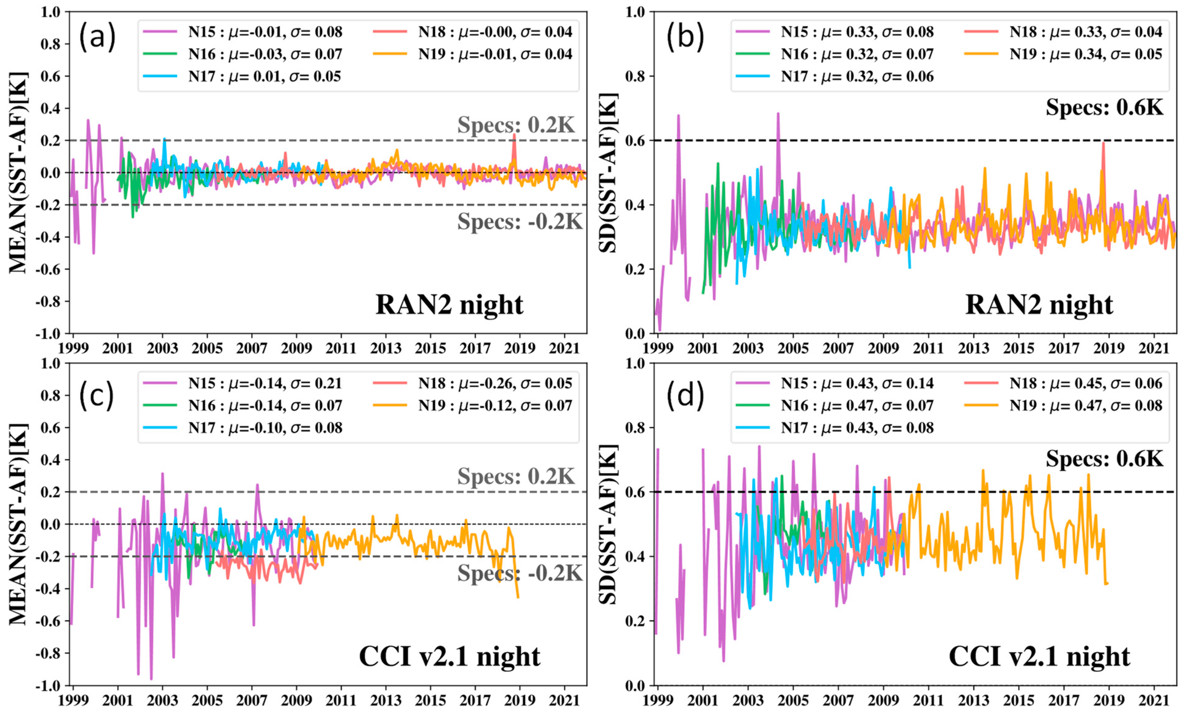
5.3. Validation of N15–N19 AVHRR/3 SSTs against AF
Figure 18 shows global monthly nighttime biases and SDs of ‘subskin’ and ‘skin’ SSTs with respect to AFs for N15–N19. In RAN2, the biases are well within the specs from 2004 onward, with mission-averaged values from −0.03 to +0.01 K. The SDs are also relatively uniform, with mission-averaged values ~0.38–0.42 K, which is only 0.01–0.03 K higher than the corresponding SDs with respect to (D + TM)’s in
Figure 15a,b. The larger scatter of biases and SDs in 1999–2005 is due to the insufficient numbers of AFs in this period (cf.
Figure 13). The CCI biases are more variable than in RAN2, with mission-averaged values being close to the (D + TM) statistics in
Figure 14d. The SDs are also more variable than in RAN2, with mission-averaged values of ~0.42–0.46 K (cf. corresponding (D + TM) values in
Figure 15d, 0.40–0.45 K).
The PF statistics in
Figure 18 exhibit features similar to those in RAN2 and CCI: the biases with respect to AFs are comparable with (D + TM) statistics in
Figure 14, with slightly larger SDs than in
Figure 15. The short-term variations in the PF statistics in
Figure 18 are noticeably smaller than in RAN2 and CCI, likely due to the PF validation MDSs including more matchups per each in situ observation, collected within a much wider ‘all night’ time window, as discussed in
Section 5.1.
Figure 19 shows the time series of biases and SDs of RAN2 and CCI ‘depth’ SSTs with respect to AF. The biases are largely consistent with those of ‘skin’ SSTs in
Figure 18. The SDs in RAN2 are smaller than the ‘skin’ SDs in
Figure 18, by 0.06–0.08 K. In CCI, the differences between ‘skin’ and ‘depth’ SDs are within ±0.01 K.
We thus conclude that the results of independent validation of the three datasets against AFs are consistent with the (D + TM) validation, in terms of both absolute values of the statistics and the relative performance of the three datasets.
6. Day–Night SST Differences
It is instructive to examine more subtle characteristics of the three datasets, such as the day–night SST differences. Recall that the SST algorithms and bands used in the three retrievals are different, and independently trained for nighttime and daytime data. In particular, the RAN2 SST was trained to minimize the global biases with respect to in situ SST. One may expect that the global day–night RAN2 SST differences would closely reproduce the diurnal differences between the corresponding daytime and nighttime in situ SSTs. It is also interesting to see how the RAN2 deltas compare with the corresponding CCI and PF results.
Figure 20 shows the time series of global monthly double differences (DDs), <
SSTday-
T0>–<
SSTnight-
T0> for RAN2, CCI, and PF SSTs. Here,
SSTday and
SSTnight are daytime and nighttime ‘subskin/skin’ SSTs in their corresponding full retrieval domains,
T0 is the first guess SST (CCI before 1 September 1991 and CMC after this date), and <..> denotes averaging over the full retrieval domains (which are different for day and night retrievals). Since
T0 is the same for day and night, it should cancel out and the
DDs should accurately estimate the globally average day–night SST difference. At the time of satellite launch,
DDs for the seven afternoon satellites in RAN2 are all about +0.2 K (for a range of LEXTs from 1:40–2:30 a.m./p.m.; cf.
Table 1); ~0 K for the mid-morning N17 (LEXT ~10 a.m./p.m.), and −0.2 K for the early morning N12/15 satellites (LEXT ~7:30 a.m./p.m.). In the course of their missions, the
DDs for different satellites change differently, following the evolution in their LEXTs (shown in
Figure 1). For instance, in 2004–2009, the DDs for N15 changed from −0.2 K to +0.2 K, as this satellite transitioned from early morning to an afternoon orbit, and then back to −0.2 in 2016–2018, after N15 returned to its early morning orbit, with close to initial LEXT. The DDs for N18 and N19 changed from +0.2 K to −0.2 K in 2017 and 2019, respectively, following their orbital evolutions.
The evolution of the CCI DDs, on average, is consistent with those in RAN2, but with somewhat larger on average magnitudes for the afternoon satellites N14 and N16–N19. It is interesting that the seasonal variations in CCI DDs for N07–N11 are very close to, albeit somewhat smaller than in RAN2, whereas, for N14–N19, the seasonal cycle is more pronounced. This may be due to different methods of (re)calibration of AVHRR BTs employed in CCI, before and after the ATSR2 launch in 1995.
The mission-averaged DDs in PF are overall consistent with those in RAN2. The notable exception is N19. The PF DDs remain flat post-2016, whereas the RAN2 N19 DDs clearly show their transition from PM to AM orbit from 2016–2019, as expected.
Overall, the time series of day–night SST differences in three datasets (with the exception of N19 in RAN2 and PF) consistently reflect long-term changes in the satellites’ orbits. More analyses are planned to refine and reconcile these initial results.
7. Conclusions
The global RAN2 SST dataset from Sep 1981–Dec 2021 was created from AVHRR GAC data of N07, N09, N11, N12, N14, N15, N16, N17, N18, and N19 with the NOAA enterprise SST system, ACSPO. The RAN2 offers two regression-based SST products, retrieved within full AVHRR swath: the ‘subskin’ SST (highly sensitive to true skin SST, but globally de-biased with respect to in situ SST), and the ‘depth’ SST (which fits in situ SST with superior accuracy and precision, but is less sensitive to true skin SST). A comparison with two other datasets produced from the NOAA AVHRR GAC L1b data, the Pathfinder v5.3, and the Climate Change Initiative v2.1, suggests the following observations.
Generally, RAN2 provides more complete data records from all available NOAA satellites, compared to both CCI and PF, and improved coverage of the global ocean with quality SST observations. This is due to performing the retrievals within the full AVHRR swath (~3000 km), using a more efficient clear-sky mask, and handling the effects of the Sun’s impingements on the AVHRR black body and the Earth view. In RAN2, the scans affected by the Sun’s impingement on the AVHRR black body are restored, whereas, in CCI, they are just filtered out. The PF dataset sometimes does not include SSTs from the periods when a given satellite could be affected by Sun impingements. The data from the most affected early morning satellites, N12 and N15, are not included in the PF. Direct comparison of CCI and PF coverages is not easy, as CCI L3C does not provide land and ice masks, and PF is only reported in L3C format.
- −
In a wider retrieval domain, the RAN2 ‘subskin’ SST provides improved performance compared with the CCI ‘skin’ SST (including smaller global biases and SDs with respect to (D + TM)’s and AFs, stability of the respective validation statistics within each mission, and their cross-mission consistency). Both RAN2 and CCI tend to provide improved performance metrics, compared with PF. However, consistent comparison of the PF performance with RAN2 and CCI is hampered by the absence of the time stamps in the PF v5.3 data files.
- −
In RAN2, SDs of ‘depth’ SST with respect to (D + TM)’s and AFs are substantially smaller compared to ‘subskin’ SDs. In contrast, the CCI SDs of ‘skin’ and ‘depth’ SSTs are very close. The margin between the CCI and RAN2 ‘depth’ SDs thus increases compared to the corresponding margins in ‘skin’ SDs. The PF does not report ‘depth’ SST. The results of independent validation of RAN2, CCI, and PF SSTs from N15 to N19 AVHRR/3s against AFs are consistent with validation against (D + TM)’s.
Although the RAN2 dataset fares well relative to the two partner’s datasets, it has room for improvement.
- −
We plan to continue extending the RAN2 dataset beyond 2021 for N15/18/19, with several months’ latency. One should remember that the orbits of these remaining NOAA satellites are unstable and often unfavorable, and their AVHRR sensors are aged and degraded, making the remaining GAC data suboptimal for SST retrievals. It is strongly recommended that ACSPO data from more recent and advanced high-resolution sensors (VIIRS, AVHRR FRAC, and MODIS) be used, in the most recent two decades. We plan to continue working towards reconciliation of AVHRR GAC SSTs with newer generation sensors, and eventually converge at one maximally consistent full SST record, from all available LEO platforms and sensors.
- −
Our analyses suggest that retrievals from the earlier N07–N11 missions remain problematic and need further analyses and improvements. This is not a simple task, as it will require multiple improvements to many elements in RAN and outside.
- −
There are indications that the quality of in situ data in the NOAA iQuam system is degraded during some periods, likely due to the degraded quality of the first guess SST used for iQuam QC. Work is underway to revisit and improve the iQuam QC, as well as the methodology of training variable regression coefficients vs. in situ data adopted in RAN.
The future work towards AVHRR 3d Reanalysis (RAN3) may also focus on the following tasks, given NOAA priorities and available resources:
- −
Analyses of the diurnal cycle in retrieved SSTs, (e.g., using the double-differences analyses employed in this study) will be continued and extended, in the context of the unstable orbits of NOAA satellites, and the retrieval algorithms may be tweaked, as needed.
- −
The improvement to the L1b calibration is by far one of the most important factors affecting the coverage of the satellite data, as well as its quality, stability, accuracy, and precision. We plan to further improve the nighttime AVHHR L1b recalibration algorithm and explore daytime L1b recalibration.
- −
We plan to carefully review and adjust the SST retrieval and cloud-masking algorithms, to minimize cloud and post-volcanic eruption aerosol leakages, and more efficiently mitigate SST regional biases.
- −
The first guess SST is a critical element of the ACSPO Clear-Sky Mask (ACSM), NLSST retrieval algorithms, and RTM input used for monitoring sensors’ brightness temperatures for stability and cross-platform consistency. Consistent, high-quality L4 analysis from September 1981–present remains an open question. The approach taken in RAN2 uses two L4 analyses: 0.05° CCI L4 prior to 1 September 1991 and 0.20° CMC L4 after that date. Our analyses suggest that the transition from one first guess to the other causes discontinuities in the time series. In the future, we will work with ACSPO L4 partners, to iteratively create and progressively improve a consistent first guess analysis, use it in ACSPO, and iterate. Efforts will be also taken to minimize the reliance of the ACSPO Clear-Sky Mask and SST retrieval algorithms on first guess SST.
- −
Some AVHRR GAC L1b data also suffer from navigation issues, especially for the earlier AVHRR/2s onboard N07/N09/N11. Although the current ACSPO processing methodology effectively processes and removes such anomalies, the coverage may be improved if those are fixed. This potential may be also explored in future RANs.
Author Contributions
Conceptualization, A.I.; methodology, B.P., V.P. and A.I.; software, V.P., B.P., Y.K. and O.J.; validation, V.P. and O.J.; formal analysis, B.P., V.P. and A.I.; investigation, B.P., V.P. and A.I.; resources, A.I.; data curation, V.P. and O.J.; writing—original draft preparation, B.P.; writing—review and editing, A.I. and V.P.; visualization, V.P.; supervision, A.I.; project administration, A.I.; funding acquisition, A.I. All authors have read and agreed to the published version of the manuscript.
Funding
This work was supported by the NOAA Ocean Remote Sensing (Paul DiGiacomo and Marilyn Yuen-Murphy, Program Managers) and NEDSIS Innovation (Mitch Goldberg, Program Manager) Programs.
Data Availability Statement
Acknowledgments
Thanks go to ORS Managers P. DiGiacomo and M. Yuen-Murphy, NESDIS Chief Scientist and Innovation Program Manager, M. Goldberg, and NOAA CoastWatch Manager V. Lance. AVHRR GAC L1b data were obtained from the NOAA STAR Central Data Repository (SCDR) operated by the STAR Data Management Working Group (DMWG). We thank Bob Kuligowski (Lead, DMWG) and Weiguo Han (Data Manager, SCDR). The views, opinions, and findings in this report are those of the authors and should not be construed as an official NOAA or U.S. government position or policy.
Conflicts of Interest
The authors declare no conflict of interest.
Abbreviations
| Acronim | Definition |
| AATSR | Advanced Along Track Scanning Radiometer |
| ACSPO | Advanced Clear-Sky Processor for Oceans |
| ACSM | ACSPO Clear-Sky mask |
| AF | Argo floats |
| ATSR/2 | Along Track Scanning Radiometer/2 |
| AVHRR | Advanced Very High-Resolution Radiometer |
| BT | Brightness temperature |
| CCI | Climate Change Initiative v2.1 |
| CMC | Canadian Meteorology Center |
| CRTM | Community Radiative Transfer Model |
| CSR | Clear-Sky ratio |
| D | Drifting buoys |
| DD | Double day–night difference |
| ESA | European Space Agency |
| FRAC | Full Resolution Area Coverage (mode) |
| GAC | Global Area Coverage (mode) |
| GDS2 | GHRSST Data Specification v.2 |
| GHRSST | Group for High Resolution SST |
| iQuam | In situ Quality Monitor |
| IR | Infrared |
| JPSS | Joint Polar Satellite System |
| LEO | Low Earth Orbiting (satellites) |
| LEXT | Local equator crossing time |
| MDS | Data set of matchups |
| MERRA | NASA Modern-Era Retrospective analysis for Research and Applications |
| MODIS | Moderate Resolution Imaging Spectroradiometer |
| NOAA | National Oceanic and Atmospheric Administration |
| NOBS | Number of observations |
| NPP | National Polar-orbiting Partnership |
| OE | Optimal estimation |
| PF | Pathfinder v. 5.3 |
| POES | Polar Operational Environmental Satellites |
| QL | Quality level |
| RAN | Reanalysis |
| RAN2 | Reanalysis Version 2 |
| S | Ships |
| SD | Standard deviation |
| SCDR | Central Data Repository |
| SQUAM | SST Quality Monitor |
| SST | Sea surface temperature |
| STAR | NOAA Center for Satellite Application and Research |
| SZA | Solar zenith angle |
| TM | Tropical moored buoys |
| VIIRS | Visible Infrared Imager Radiometer Suite |
| VZA | Satellite view zenith angle |
References
- Kalluri, S.; Cao, C.; Heidinger, A.; Ignatov, A.; Key, J.; Smith, T. The Advanced Very High Resolution Radiometer: Contributing to Earth Observations for over 40 Years. Bull. Am. Meteorol. Soc. 2021, 102, E351–E366. [Google Scholar] [CrossRef]
- Ignatov, A.; Zhou, X.; Petrenko, B.; Liang, X.; Kihai, Y.; Dash, P.; Stroup, J.; Sapper, J.; DiGiacomo, P. AVHRR GAC SST Reanalysis Version 1 (RAN1). Remote Sens. 2016, 8, 315. [Google Scholar] [CrossRef] [Green Version]
- Kilpatrick, K.A.; Podestá, G.P.; Evans, R. Overview of the NOAA/NASA advanced very high resolution radiometer Pathfinder algorithm for sea surface temperature and associated matchup database. J. Geophys. Res. Space Phys. 2001, 106, 9179–9199. [Google Scholar] [CrossRef]
- Saha, K.; Zhao, X.; Zhang, H.; Casey, K.S.; Zhang, D.; Baker-Yeboah, S.; Kilpatrick, K.A.; Evans, R.H.; Ryan, T.; Relph, J.M. AVHRR Pathfinder Version 5.3 Level 3 Collated (L3C) Global 4 km Sea Surface Temperature for 1981-Present. NOAA National Centers for Environmental Information. 2018. Available online: https://doi.org/10.7289/v52j68xx (accessed on 14 June 2022).
- Merchant, C.J.; Embury, O.; Bulgin, C.E.; Block, T.; Corlett, G.K.; Fiedler, E.; Good, S.A.; Mittaz, J.; Rayner, N.A.; Berry, D.; et al. Satellite-based time-series of sea-surface temperature since 1981 for climate applications. Sci. Data 2019, 6, 223. [Google Scholar] [CrossRef] [Green Version]
- ESA Climate Office. Available online: https://climate.esa.int/en/projects/sea-surface-temperature/data/ (accessed on 14 June 2022).
- Global Climate Observing System. Available online: https://gcos.wmo.int/en/essential-climate-variables/table (accessed on 14 June 2022).
- Jonasson, O.; Ignatov, A.; Pryamitsyn, V.; Petrenko, B.; Kihai, Y. JPSS VIIRS SST Reanalysis Version 3. Remote Sens. 2022. submitted. [Google Scholar]
- Pryamitsyn, V.; Petrenko, B.; Ignatov, A.; Kihai, Y. Metop First Generation AVHRR FRAC SST Reanalysis Version 1. Remote Sens. 2021, 13, 4046. [Google Scholar] [CrossRef]
- Petrenko, B.; Ignatov, A.; Kihai, Y.; Heidinger, A. Clear-Sky Mask for the Advanced Clear-Sky Processor for Ocean. J. Atmos. Ocean. Technol. 2010, 27, 1609–1623. [Google Scholar] [CrossRef]
- Petrenko, B.; Ignatov, A.; Kihai, Y.; Stroup, J.; Dash, P. Evaluation and selection of SST regression algorithms for JPSS VIIRS. J. Geophys. Res. Atmos. 2014, 119, 4580–4599. [Google Scholar] [CrossRef]
- Petrenko, B.; Ignatov, A.; Kihai, Y.; Dash, P. Sensor-Specific Error Statistics for SST in the Advanced Clear Sky Processor for Ocean. J. Atmos. Ocean. Technol. 2016, 33, 345–359. [Google Scholar] [CrossRef]
- Petrenko, B.; Pryamitsyn, V.; Ignatov, A.; Kihai, Y. SST and cloud mask algorithms in reprocessing 1981–2002 NOAA AVHRR data for SST with the Advanced Clear-Sky Processor for Oceans (ACSPO). Proc. SPIE 2020, 11420. Available online: https://spie.org/Publications/Proceedings/Paper/10.1117/12.2558660 (accessed on 30 June 2022).
- Petrenko, B.; Pryamitsyn, V.; Ignatov, A. Filtering cold outliers in SSTs retrieved from early AVHRRs for the second AVHRR GAC reanalysis. Proc. SPIE 2022, 1175205. [Google Scholar] [CrossRef]
- Petrenko, B.; Pryamitsyn, V.; Ignatov, A.; Kihai, Y. Mitigation of the AVHRR instrumental issues in historical SST retrievals for the NOAA AVHRR GAC SST RAN2. In Proceedings of the Ocean Sensing and Monitoring XIV, Orlando, FL, USA, 3–7 April 2022; Volume 1211803. [Google Scholar] [CrossRef]
- Pryamitsyn, V.; Ignatov, A.; Petrenko, B.; Jonasson, O.; Kihai, Y. Evaluation of the initial NOAA AVHRR GAC SST Reanalysis Version 2 (RAN2 B01). Proc. SPIE 2022, 11420. Available online: https://spie.org/Publications/Proceedings/Paper/10.1117/12.2558751?SSO=1 (accessed on 30 June 2022).
- Xu, F.; Ignatov, A. Evaluation of in situ sea surface temperatures for use in the calibration and validation of satellite retrievals. J. Geophys. Res. Earth Surf. 2010, 115, C09022. [Google Scholar] [CrossRef]
- Xu, F.; Ignatov, A. In Situ SST Quality Monitor (iQuam). J. Atmos. Ocean. Technol. 2014, 31, 164. [Google Scholar] [CrossRef]
- In Situ SST Quality Monitor (iQuam). Available online: https://www.star.nesdis.noaa.gov/socd/sst/iquam/ (accessed on 14 June 2022).
- Xu, F.; Ignatov, A. Error characterization in iQuam SSTs using triple collocations with satellite measurements. Geophys. Res. Lett. 2016, 43, 10826–10834. [Google Scholar] [CrossRef]
- Dash, P.; Ignatov, A.; Kihai, Y.; Sapper, J. The SST Quality Monitor (SQUAM). J. Atmos. Ocean. Technol. 2010, 27, 1899. [Google Scholar] [CrossRef]
- SST Quality Monitor (SQUAM). Available online: https://www.star.nesdis.noaa.gov/socd/sst/squam/ (accessed on 14 June 2022).
- He, K.; Ignatov, A.; Kihai, Y.; Cao, C.; Stroup, J. Sensor Stability for SST (3S): Toward Improved Long-Term Characterization of AVHRR Thermal Bands. Remote Sens. 2016, 8, 346. [Google Scholar] [CrossRef] [Green Version]
- Sensor Stability for SST (3S). Available online: https://www.star.nesdis.noaa.gov/socd/sst/3s/ (accessed on 16 June 2022).
- Cao, C.; Weinreb, M.; Sullivan, J. Solar contamination effects on the infrared channels of the advanced very high resolution radiometer (AVHRR). J. Geophys. Res. Earth Surf. 2001, 106, 33463–33469. [Google Scholar] [CrossRef]
- Trishchenko, A.; Fedosejevs, G.; Li, Z.; Cihlar, J. Trends and uncertainties in thermal calibration of AVHRR radiometers onboard NOAA-9 to NOAA-16. J. Geophys. Res. Earth Surf. 2002, 107, ACL-17. Available online: https://agupubs.onlinelibrary.wiley.com/doi/abs/10.1029/2002JD002353 (accessed on 30 June 2022). [CrossRef] [Green Version]
- Reynolds, R.W. Impact of Mount Pinatubo Aerosols on Satellite-derived Sea Surface Temperatures. J. Clim. 1993, 6, 768–774. [Google Scholar] [CrossRef]
- Merchant, C.; Harris, A.R.; Murray, M.J.; Závody, A.M. Toward the elimination of bias in satellite retrievals of sea surface temperature: 1. Theory, modeling and interalgorithm comparison. J. Geophys. Res. Earth Surf. 1999, 104, 23565–23578. [Google Scholar] [CrossRef]
- Walton, C.C.; Pichel, W.G.; Sapper, J.F.; May, D.A. The development and operational application of nonlinear algorithms for the measurement of sea surface temperatures with the NOAA polar-orbiting environmental satellites. J. Geophys. Res. Earth Surf. 1998, 103, 27999–28012. [Google Scholar] [CrossRef]
- Brasnett, B.; Colan, D. Assimilating retrievals of sea surface temperature from VIIRS and AMSR2. J. Atmos. Ocean. Technol. 2016, 33, 361–375. [Google Scholar] [CrossRef]
- Liang, X.; Ignatov, A.; Kihai, Y. Implementation of the Community Radiative Transfer Model (CRTM) in Advanced Clear-Sky Processor for Oceans (ACSPO) and validation against nighttime AVHRR radiances. J. Geophys. Res. Earth Surf. 2009, 114, D06112. [Google Scholar] [CrossRef]
- Rienecker, M.M.; Suarez, M.J.; Gelaro, R.; Todling, R.; Bacmeister, J.; Liu, E.; Bosilovich, M.G.; Schubert, S.D.; Takacs, L.; Kim, G.K.; et al. MERRA: NASA’s Modern-Era Retrospective Analysis for Research and Applications. J. Clim. 2011, 24, 3624. Available online: https://www.jstor.org/stable/26191103 (accessed on 30 June 2022). [CrossRef]
- Modern-Era Retrospective analysis for Research and Applications (MERRA). Available online: https://gmao.gsfc.nasa.gov/reanalysis/MERRA/ (accessed on 14 June 2022).
- The Group for High Resolution Sea Surface Temperature Science Team; Casey, K.; Donlon, C. The Recommended GHRSST Data Specification (GDS). Available online: https://zenodo.org/record/4700466#.Yr0ZVuxBxPZ (accessed on 30 June 2022).
- Merchant, C.; Le Borgne, P.; Roquet, H.; Legendre, G. Extended optimal estimation techniques for sea surface temperature from the Spinning Enhanced Visible and Infra-Red Imager (SEVIRI). Remote Sens. Environ. 2013, 131, 287–297. [Google Scholar] [CrossRef]
- Merchant, C.J.; (University of Reading, Reading, UK). Personal communication, 13 February 2020.
- Jonasson, O.; Gladkova, I.; Ignatov, A.; Kihai, Y. Algorithmic improvements and consistency checks of the NOAA global gridded super-collated SSTs from low Earth orbiting satellites (ACSPO L3S-LEO). Proc. SPIE 2021, 11752. Available online: https://spie.org/Publications/Proceedings/Paper/10.1117/12.2585819?SSO=1 (accessed on 30 June 2022).
| Publisher’s Note: MDPI stays neutral with regard to jurisdictional claims in published maps and institutional affiliations. |
© 2022 by the authors. Licensee MDPI, Basel, Switzerland. This article is an open access article distributed under the terms and conditions of the Creative Commons Attribution (CC BY) license (https://creativecommons.org/licenses/by/4.0/).


 ,
, 


