1. Introduction
A solar eclipse is a natural phenomenon that occurs when the Moon moves in the way between the Sun and Earth, totally or partially blocking the Sun, casting a shadow over the Earth. Since the Sun is one of the major drivers of atmospheric effects, such as its ionization at high altitudes, its blocking produces several disturbances. The atmospheric effects of a solar eclipse have been the subject of extensive research, mainly in meteorological parameters, total column ozone, photochemistry, gravity waves, and ionospheric parameters [
1]. Despite the large number of studies concerning eclipses, the event of a solar eclipse is still unique since it happens at different seasons, different times of the day, different locations, and under different synoptic and geomagnetic conditions [
1,
2,
3]. In addition, with every new eclipse, the scientific community gains larger numbers and a variety of instruments, which allow us to revisit the proposed conclusions from previous eclipses.
The ionosphere is directly affected since this atmospheric layer is produced by solar radiation. The total electron content (TEC) is a measure of the electron density in the ionosphere integrated along the line of sight, thus, an indication of its ionization. TEC can be obtained using a radio link between a satellite and the ground. Nowadays, the most common system delivering TEC measurements is the Global Navigation Satellite Systems (GNSS), which requires TEC measurements to improve the precision of position estimation. TEC is expressed in TEC units (TECu), where
. The perturbation of the ionosphere can be analyzed through the variations of TEC. The main parameters of the TEC variations during the eclipses are the delay value (
) relative to the maximum phase of the eclipse; its amplitude (A), which generally is a decrease; and the duration (
) of the perturbation [
4]. Since the Moon’s shadow moves rapidly from west to east across the Earth at supersonic speed, the total eclipse lasts just a few minutes anywhere [
5,
6,
7]. Previous works have reported the depletion of TEC after the onset of the partial solar eclipse and have presented values of A in percent (A[%]) that can reach up to −64% with
from −30 to 180 min [
8,
9,
10,
11]. This delay has been interpreted as an indicator of the combined effect of the photochemical processes and plasma dynamics [
1,
12]. Some works have reported
from 50 to 240 min [
4,
13]. However, some studies have reported even longer effects [
14,
15]. A historical summary of ionospheric responses to solar eclipses since 1920 can be found in the Appendix in Bravo et al. [
16].
Recent studies have shown that the effects of a solar eclipse on the ionosphere are not only local but can affect other geographic regions outside the umbra/penumbra of the eclipse [
15,
17,
18,
19,
20]. These effects may be due to transport between hemispheric magnetic conjugates, alteration of the equatorial fountain effect, generation of a disturbed dynamo, and/or Atmospheric Gravity Waves (AGWs) that generate Traveling Atmospheric Disturbances (TADs) and/or Traveling Ionospheric Disturbances (TIDs).
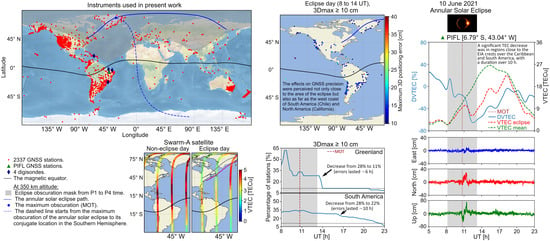
An annular solar eclipse took place on 10 June 2021. The first external contact (P1 time) and the last external contact (P4 time) of the solar eclipse were at 08:12:22 UT and 13:11:22 UT, respectively. The partial solar eclipse was seen from the following geographic regions: in parts of the eastern United States and northern Alaska, Canada and parts of the Caribbean, Europe, Asia, and northern Africa. The annular eclipse was visible from parts of northeastern Canada, Greenland, and the Arctic Ocean, passing through the North Pole, and ending in Russian territory. It maximum magnitude was 0.944: this is the fraction of the angular diameter of a celestial body being eclipsed. This magnitude value was reached at geographic coordinates 80.815°N, and 66.78°W, at 10:41:57 UT (Greatest Eclipse time, GE time,
http://xjubier.free.fr/en/site_pages/solar_eclipses/ASE_2021_GoogleMapFull.html, last accessed on 15 June 2022). The paths at ground level and at 350 km of altitude of the annular eclipse are shown in
Figure 1 (see
Supplementary Materials, Video S1). Due to the specific geometry of each eclipse, the paths differ both geographically and temporally according to the height considered, which could be significant when analyzing them [
21].
Solar eclipses are rare events and, particularly, the 10 June 2021 event is an excellent opportunity to study the eclipse-induced effects on the polar ionosphere. Since the ionospheric variations can perturb GNSS, the eclipse can be used to study the positioning errors in these regions. There are some studies on the effects of the ionosphere during solar eclipses over the northern polar region. One of the first reported ones was the total solar eclipse that occurred on 9 March 1997 over Kazakhstan, Mongolia, eastern Siberia, and the Arctic Ocean (
to 180 min and A = −5 TECu) [
4,
22]. Another reported one is the total solar eclipse that occurred on 1 August 2008 over Canada, northern Greenland, the Arctic Ocean, central Russia, Mongolia, and China (
= −27 to 44 min, and A[%] = −40 to −11%) [
10]. The most recent one is the eclipse that occurred on 20 March 2015 that covered the North Atlantic, Faroe Islands, and Svalbard (A[%] = −50 to −10%) [
5,
23]. This last one happened during the recovery phase of the most intense geomagnetic storm during Solar Cycle 24, the so-called St. Patrick’s Day Storm. Due to the limited availability of GNSS stations around the globe at the time of these previous studies, they were focused on a regional scale. The increasing number of accessible GNSS stations around the world allows a study on a global scale, facilitating the search of potential interactions between regions. This can show how spreadable GNSS disturbances are. In particular, the poles are of interest since several ionospheric disturbances can start from there during geomagnetic storms.
In GNSS receivers, TEC is estimated simultaneously from several satellites of the network, which serves to study the ionosphere. (e.g., [
4,
8,
24], among many others). During the eclipses, the ionization decreases, producing a depletion in TEC. Although a decrease in electron concentration during a solar eclipse could produce an improvement in the positioning precision, it actually generates positional errors [
25,
26]. Few authors have analyzed the GNSS positioning errors caused by the influence of solar eclipses. The eclipses that occurred over Croatia on 11 August 1999 [
27], over China on 22 July 2009 [
28], and over the United States on 21 August 2017 [
26] are some of the studies that analyzed GNSS positioning errors.
For the 1999 solar eclipse, Filjar, et al. [
27] used a single frequency receiver located in the north of Croatia with ∼95% of maximum percentage of obscuration (MPO). In this work the authors did not relate ionospheric disturbances with positioning variations. The authors collected the horizontal positioning at the eclipse’s maximum obscuration time (MOT). They calculated an average positioning error of ∼34 m on horizontal Global Positioning System (GPS) accuracy for that time. These horizontal values could be due to the use of a single-frequency, the number of receiver channels, and the possible influence of Selective Availability (until May 2000).
Jia-Chun et al. [
28] used eight GPS stations to study the TEC changes and their effect on the positioning during the 22 July 2009 solar eclipse. They possessed a real-time point positioning and real-time precision of single baselines. The measurements were affected by a geomagnetic storm (Dst peak = −80 nT and Kp-index =
), which made it difficult to separate the influence of the eclipse from the storm one.
In the case of the 2017 eclipse, Park et al. [
26] computed and compared the rate of change of the TEC (ROT) with respect to the day before and the day after the eclipse; and with a time window of 3 h, from 16 UT. They determined the means of positioning errors at four GNSS stations (localized in Oregon, United States) within the path of the total solar eclipse which reached ∼32 cm. However, on reference days, the means of positioning errors were between 7–14 cm. The authors used the average length of the eight baselines, which was ∼270 km. On the eclipse day, the means of positioning results were −4 to 324% over the day before and the day after the eclipse. Yuan et al. [
25] established the ionospheric eclipse factor method (IEFM) to model the ionospheric delay searching for the improvement of the GNSS positioning estimation. In this contest, the paper introduces the concept of the ionospheric eclipse factor method for the IPP for relatively precise separation of daytime from nighttime for the ionosphere. Although the ionospheric eclipse factor is not related to a solar eclipse as an astronomical phenomenon that occurs when the Moon obscures the Sun from Earth, this method could be used in future studies related to the impact of solar eclipses on GNSS positioning.
In our case, we obtain the apparent position variation using the post-processing kinematic precise point positioning (PPP) with ambiguity resolution (PPP-AR) mode. We chose this method because PPP demonstrates a high ability to improve position estimation. PPP is used for calculating the coordinates of a single receiver without the need for a reference station nearby as a control station. In addition, we can find some free PPP services available online [
29]. PPP-AR is an enhanced version of the PPP technique that resolves the carrier phase ambiguities, improving the PPP accuracy [
29,
30,
31]. Katsigianni et al. [
30] recently presented a comparison between PPP and PPP-AR. In order to offer the community the possibility of evaluating our analysis, we used an online service. Thus, we selected the CSRS-PPP service for this work because it is one of the most commonly used PPP online services in the field. We also applied the common noise filter to more than 2300 GNSS stations, to correct the time series of the North, East, and Up components of the GNSS receivers, as described in [
29].
The regular ionospheric effects of solar eclipses are not yet fully understood. Studies of the eclipse-induced effects on the ionosphere are important because they provide a better understanding of the processes that control the ionosphere and that can cause GNSS positioning errors. In the present paper, we present the impact of the 10 June 2021 annular solar eclipse on ionospheric variations that also cause errors in GNSS positioning. Therefore, we first analyze the ionospheric behavior at a global scale based on 2337 dual-frequency (DF) GNSS stations, Swarm-A satellite, and four ionospheric stations. We used GNSS stations distributed around the world since they will allow us to evaluate the effects beyond the northern polar region with a higher spatial resolution than ever before. Unlike previous studies about the GNSS positioning errors caused by the influence of solar eclipses, our study is focused on a global scale. This allowed us to find other locations in the world that could be affected by a perturbation in the north pole and how that perturbation propagates to those potential locations.
3. Results
In this section, we present the main results obtained after applying the methodology described in the previous section. The results obtained in this work can be divided into two main parts: (1) the analysis of the TEC maps that present the effects on the ionosphere at a global scale; and (2) the calculation of the positioning errors that these ionospheric effects generate.
3.1. Ionospheric Behavior and TEC Maps
From the data of each station, we can estimate the VTEC for each station during the selected period of days. By using the ordinary Kriging interpolation, as described in
Section 2.1, it is possible to obtain VTEC maps.
Figure 3 shows a summary of the TEC maps by contrasting the eclipse (VTECe) and control (
) days. We present some particular hours: 09.15 UT, 10.70 UT (GE time), 12.00 UT, 13.19 UT (P4 time), 13.72 UT (P4 time
0.5 h), and 17.66 UT.
Figure 3 also shows the eclipse masks from 20% obscuration and with intervals of 20%, at 350 km altitude (white line). From these figures, it is possible to notice that the Greenland and South American sectors are two of the most affected in terms of VTEC depletion. VTECe in IPP and DVTEC[TECu] in
Figure 3 use the Kriging interpolation method and are shown in equidistant cylindrical projection and Northern Hemisphere polar plots (see
Supplementary Materials, Figure S1).
The 09.15 UT, 12.00 UT, and 13.72 UT maps were chosen in particular because they show the greatest apparent position variations during the eclipse time window. The 17.66 UT map was chosen because the ionosphere was roughly recovered by that time. For a better visualization of the eclipse effects, a third column has been incorporated where the VTEC differential in TEC units (DVTEC[TECu]) is shown.
DVTEC had values of around −20% (−2 TECu) over the oceanic sectors when the eclipse began (P1-time). However, at these locations, the GNSS receivers are scarce, which can cause less reliable interpolation. This value could be considered as part of the non-significant variations in DVTEC. A similar problem is identified over Central Africa, where there is a value of 50% (7 TECu), possibly also due to the few receivers in this area (see
Figure 1). The anomalies in these areas were observed more than 5 h before the eclipse. We will focus mainly on changes generated over the continental areas of America and Europe, while the other areas will not be considered for this analysis.
When the ionospheric TEC effects due to eclipse have already begun, the 09.15 UT maps show a slight depletion of
(
TECu) across eastern Canada under the shadow of the eclipse. At 10.70 UT (GE-time), these changes expand beyond the shadow area of the eclipse (see second row of
Figure 3). The 10.70 UT maps show that ionospheric TEC depletion did not only occur across the obscuration region over the Northern Hemisphere. DVTEC[%] had values of around −60% (−4 to −2.5 TECu) over the South and East coasts of Greenland,
(
TECu) eastern Canada, and around −50% (∼−3 TECu) over the Lesser Antilles.
The 12.00 UT, 13.19 UT, and 13.72 UT maps show DVTEC[%] had values of around −30% (−3 to −1.5 TECu) over Russia after GE time.
Figure 3) also illustrates how the TEC disturbance moved from West to East over the Northern Hemisphere, following the path of the annular solar eclipse. At 12 UT, there is a recovery of the ionospheric TEC over Canada and Greenland regions, but DVTEC[%] had values of less than −50% in East coast of Greenland. Ionospheric TEC depletion had values of around −60% (∼−5 TECu) over the Lesser Antilles near the north crest of Equatorial Ionization Anomaly (EIA) and less than −30% (∼−5 TECu) appeared over South America near the south crest of EIA. The 13.19 UT and 13.72 UT maps show another slight recovery of the ionospheric TEC in the North Atlantic and Greenland, as well as a TEC depletion over Russia. Moreover, TEC depletion was accentuated in the EIA crests over South America, where DVTEC[%] had values of less than −60% (<
TECu). It is shown that the effects lasted beyond the end of the eclipse.
The 17.66 UT maps present the global recovery of the ionosphere a few hours after the end of the eclipse. These maps show a slight DTEC[%] enhancement in the center of the EIA form ∼−16% to ∼10%. But the TEC depletion was ∼−20% (−5 to −3 TECu) in the EIA crest over South America. The TEC behavior in the EIA crests was maintained until after 19.66 UT.
On the other hand, DoY 162 had geomagnetic activity (see
Section 2.5). Therefore, we checked if the DVTEC changes that we observed for the day of the eclipse were due to using DoY 162 as one of the reference days. We compute a new
(
, Equation (
1)), and a new
by averaging the VTEC values at the same time of the day,
t, for the reference days, DoYs 159, 160, and 163. For each map, we used the map algebra (
). The mean value ranged between −0.5 and 0.1 TECu, with a standard deviation of less than 0.7 TECu (see
Supplementary Materials, Figure S2, Table S1). Therefore, geomagnetic activity during the DoY 162 did not cause problems in the background to our ionospheric TEC results for the eclipse day.
Ionospheric Behavior Using Swarm Satellite Measurements
We also present ionospheric behavior using Swarm-A measurements (see
Figure 4). We illustrate VTEC at 850 km altitude on DoY 161 compared to DoY 159 during three ascending passes of the Swarm-A satellite (⩾45°S, see
Figure 4 (upper panels)). We selected the three Swarm-A satellite passes that best fit the eclipse region and eclipse time window. The first satellite pass (∼8.50–9.20 UT) occurred after P1 time. The greatest ionospheric TEC degradation was −30°S–30°N (∼
TECu,
). The second pass (∼10.10–10.80 UT) was close to the GE time. As latitude increases, TEC decrease. The third satellite pass (∼11.70–12.40 UT) was performed prior to P4 time (∼
TECu,
). It is possible to see that TEC decrement was concentrated between 10 and 30°N (VTEC was close to ∼−1 TECu, and ∼−30%). Ionospheric TEC depletion was greatest in the 15–75°N region (∼
TECu,
).
Figure 4 (bottom panels) depict in situ
measurements made by Swarm-A Langmuir probe.
Figure 4 (upper panels) show that VTEC behaves similarly to
. We observed that
decrease was −46% (
e/cm
3) at ∼8.86 UT in ∼1°N; −55% (
e/cm
3) at ∼10.62 UT in ∼50°N; and −55% (
e/cm
3) at ∼12.05 UT in ∼20°N.
3.2. ROTI and GNSS Precise Point Positioning Accuracy Maps
We estimated the ionospheric TEC, ROTI, and positioning for the full 5 days but only show 6 hours per day. On the eclipse day, we observe the largest positioning variations during this time window (around P1–P4 time, see
Figure 5). This study focuses on the positioning accuracy of the stations during the 10 June 2021 annular solar eclipse, during the time between 8 and 14 UT. We estimated the PPP-AR using the CSRS-PPP service, as described in
Section 2.4. Comparing the eclipse day with respect to the DoYs 159 and 160, we can see that the percentage of GNSS stations that exceeded maximum 3D positioning error ⩾10 cm and 3D-RMS ⩾3 cm (positioning thresholds) jumped from ∼180 (∼8%) to 333 (∼14%) and from ∼170 (∼7%) to 210 (∼9%), respectively. In addition, the ROTI threshold ⩾0.25 TECu/min was taken according to Liu et al. [
36], and used in the methodology [
29].
Figure 6 shows maximum 3D positioning errors, 3D-RMS of the apparent position, and ROTI maps, for each of the five selected DoYs.
ROTI was calculated as described in
Section 2.2 to study the relationship between the variation of TEC and the positioning error for the eclipse. The images in the
Figure 6 (right panel) show five maps of ROTI, each representing the stations that had ROTI greater than 0.25 TECu/min. Each map represents a different day, but at the same time as that of the solar eclipse, DoYs 160–163 between 8 and 14 UT. We do not show the maps for DoY 159 because they are similar to those for DoY 160.
The TEC data (e.g.,
Figure 3) and the derived PPP-AR (see
Figure 6 (left panels)), and
Figure 7) show that there are two regions where the errors are more severe during the solar eclipse (DoY 161, between 8 and 14 UT). These regions are Greenland and South America. For this reason, we focused this study on these sectors.
In the Greenland and South America regions, we can find 36 (∼2%) and 335 (∼14%) of the 2337 total available GNSS stations, respectively. We determined the percentage of stations localized in both regions that had errors that fell at certain intervals during the time period of the annular eclipse (between 8 and 14 UT).
Figure 7 shows the percentages of stations that meet the thresholds of maximum 3D positioning error, 3D-RMS, and ROTI. We determined the number of GNSS stations based on ROTI activity and positioning values (see
Supplementary Materials, Tables S2–S4, where each column in these tables represents the percentage of stations with maximum 3D position error, 3D-RMS, and ROTI at certain intervals in the selected period).
Figure 5 shows in more detail the percentage of stations with maximum 3D errors ⩾10 cm on eclipse day. In Greenland, during the inicial period of the eclipse (∼P1 time), the percentage of stations with maximum 3D positioning error rises to 60%. Subsequently, the value remains at ∼28% until it increases to ∼33% between 10.5 and 11.25 UT (around GE time). The value then returns to ∼28% until 14 UT (after P4 time), when it drops to ∼11% of stations. In South America, the percentage of stations with maximum 3D positioning error had a maximum of ∼34% between 9.75 and 11.5 UT (around GE time). We also were able to observe a decrease in stations that exceeded the threshold maximum 3D positioning error from ∼28% to ∼22% between 16 and 17 UT.
3.3. Ionospheric Behavior and GNSS Positioning Errors by Region
To study the effects of the eclipse, we selected 24 stations from among the 2337 GNSS stations (see
Figure 1). We chose five GNSS stations close to the annular solar eclipse (KMOR, KAGZ, MARG, IQAL, PICL). There were six GNSS stations located in the partial eclipse region (CN00, TRO1, SVTL, TIXI, MAG0, YAKT). Furthermore, we used five stations located in the Caribbean and South America (LMMF, BOAV, PIFL, MSBL). The sunrise (in PICL and CN00 stations) and the sunset (in MAG0 and YAKT stations) happened during the eclipse time window at ground level but did not take place at the ionospheric height of 350 km. More details about the GNSS stations and eclipse conditions (with respect to the ionospheric height of 350 km) can be found in
Table 1.
Figure 8 presents the results of ionospheric TEC of 12 stations from among the 24 selected GNSS stations for the eclipse day (VTECe), the reference days (
), and the final results of DVTEC [%]. The vertical blue shaded region between P1 time and P4 time, with GE time (brown dotted line). The vertical yellow shaded region between C1 time and C4 time, with MOT (black dotted line). Each plot is shown between 5 and 23 UT. The maximum reduction values of TEC for each station are indicated in
Table 1 (
= 1 to 288 min, and A[%]= −65 to −27%). This eclipse occurred during the morning at most of the selected stations but took place in the afternoon at five stations (NYA1, TRO1, SVTL, TIXI, MAG0, YAKT). The Sun’s activity became stronger around noon and the clear TEC reduction during the eclipse can be observed. The stations that are near the path of the annular eclipse at 350 km altitude and the east coast of Greenland reached lower values of DVTEC [%] ∼−55% than the stations with the annular eclipse at the surface level DVTEC [%] ∼−40%.
Figure 8 shows the ionospheric TEC changes for 12 of the 24 GNSS stations presented in
Table 1. The TEC disturbance lasted longer at the GNSS stations located in South America and the Lesser Antilles (CN00, LMMF, CN57, BOAV, PIFL, MSBL). In these GNSS stations, the ionospheric effect caused by the eclipse started at ∼8.5–9 UT and ended ∼18–21 UT (
> 10 h). The ionospheric response is similar in BOAV and MSBL stations where A[%] ∼−30%. In MAG0, TIXI, and YAKT stations, we observe a TEC depletion during the eclipse time window, but it is not as noticeable as in the other cases.
Additionally, the number of GNSS stations according to ROTI activity was: 5 strong (BLAS, PIFL, LEFN, NYA1, and MARG stations), 2 moderate (KMOR and KAGZ stations) and 17 without activity (see
Table 1).
In the same way, we presented the results of PPP-AR of 24 DF-GNSS stations during eclipse day. The time series were corrected for the common noise filter of the East, North, and Up components. The stations had variations in position within the time window of the eclipse (between 8 and 14 UT). The station with the highest positioning errors in the East, North, and Up components was PIFL stations. KAGA, GLS2, SENU, and MSBL stations also showed position variations between 5 and 8 UT.
Equation (
6) is used to obtain the 3D results. Then, the maximum 3D positioning error and 3D-RMS values (between 8 and 14 UT) for each station are indicated in
Table 1. We note that the GNSS stations can be separated according to the percentage of maximum 3D positioning error and 3D-RMS, with respect to the maximum values of reference days.
In the case of maximum 3D positioning error, four stations presented values below 0% (MARG, ALGO, CN00, and LMMF); eight 0–25% (KAGZ, IQAL, BLAS, BOAV, NYA1, SVTL, MAG0, and YAKT); seven GNSS stations were between 25 and 50%; three stations were 60–70% (GLS2, KUAQ, and SENU); and two stations > 100% (PIFL and TRO1).
On the other hand, for 3D-RMS in a percentage, 1 station was < 0% (CN00); 11 stations were 0–25% (KAGZ, MARG, LEFN, BLAS, KAGA, GLS2, KUAQ, NYA1, SVTL, TIXI, and YAKT); 7 stations were 25–50% (KMOR, IQAL, ALGO, LMMF, CN57, PIFL, and MSBL); 3 stations were 75–100% (SENU, PICL, and BOAV); and 2 stations > 100% (TRO1 and MAG0).
A Case Study
We will describe in more detail the results obtained with PIFL GNSS station (6.79°S, 43.04°W). PILF had the largest ionospheric disturbances and GNSS positioning errors (see
Table 1). TEC depletion had values around −65% (−11.8 TECu) at 110 min after GE time (see
Figure 8).
Figure 9 presents the ionospheric behavior (ROT, ROTI) and kinematic DF-GNSS PPP-AR mode during DoYs 160–163 between 5 and 23 UT. We do not show DoY 159 because it does not differ significantly from DoY 160.
Figure 9 (left, middle panels) illustrates examples of GPS ROT and GPS ROTI variations along with all visible GPS satellites. On eclipse day, we can observe a |ROT| > 1.5 TEC/min in eight Pseudo Random Noises (PRN-4, 7, 8, 9, 14, 27, 28, 30). The |ROT| value was exceeded by 3–4 PRNs during the reference DoYs 159, 160, and 163. In contrast, the |ROT| was exceeded by seven PRNs on DoY 162 (see
Figure 9 (left panels)). On DoY 161 between 10.66 and 17.39 UT (6.73 h), we could note 22 and 8 ROTI values >0.5 and >1 TECu/min, respectively (see
Figure 9 (middle panels)). The ROTI peak was 1.9 TECu/min at 12.75 UT, estimated from the PRN-4. On this day, nine PRNs (PRN-4, 7, 8, 9, 10, 14, 27, 28, 30) presented a moderate and/or strong ROTI activity. Regarding DoYs 159, 160, 162 and 163, we observed 12, 8, 20 and 6 values with moderate and/or strong ROTI activity. Then, this station showed strong TEC activity during each of the five DoYs. The ROTI value was higher on eclipse day 1.9 TECu/min at 12.76 UT (∼25 min after P4 time).
Figure 9 (right panels) show the apparent position variation of kinematic DF-GNSS PPP-AR mode in the East, North, and Up components for the PIFL GNSS station. These time series has been corrected for the common noise filter. On DoY 161, the apparent peak ground displacement in the East, North, and Up components were 18, 40, and 119.8 cm, respectively. Moreover, the maximum 3D positioning error ⩾10 cm ∼9.80 UT by ∼3.30 h. The Up, North, and East components are ordered from highest to lowest errors. Then, positioning errors in the three components and their results were clear during the eclipse time window (after GE time), relative to the reference days.
4. Discussion
In this section, we discuss the main findings regarding the 10 June 2021 annular solar eclipse. The main goal is to study the positioning errors of GNSS receivers caused by this solar eclipse. In order to verify our findings, we compare our ionospheric values with results presented for other solar eclipses over the northern polar region (9 March 1997 [
4,
22]; 1 August 2008 [
10]; and 20 March 2015 [
5,
23]).
There are several free-to-use software available for single-station TEC estimation methods [
47,
48]. We selected GPS-TEC software because it is a widely used method by the scientific community to study phenomena such as geomagnetic storms [
29] and solar eclipses [
49], among others. GPS-TEC software is fundamentally based on the assumption that ionospheric density depends on altitude to determine VTEC from STEC.
4.1. Ionospheric Behavior
The present analysis aims to show, as best as currently possible, the effects that the solar eclipse generates both in the ionosphere under the moon’s shadow as well as in the global ionosphere. The relevance of this event is that there are few of them that occur in polar regions, in this case, in the Arctic.
We have used interpolated global maps from TEC and we have calculated the difference between eclipse and reference days. The results of the TEC maps show a significant reduction under the moon’s shadow, except at the CN00 station that has similar behavior to the LMMF, CN57, BOAV, and MSBL stations (see
Figure 3 and
Figure 8,
Table 1); the GNSS stations located in the region of the eclipse reaching a maximum of
= 1 to 288 min, A peak ∼−5 TECu, A[%] = −61 to −27%.
Table 1 details these parameters for GNSS stations of some selected regions (see
Figure 1). The values of these parameters agree with those obtained for the solar eclipses of 9 March 1997 solar eclipse [
4,
22], 1 August 2008 [
10], and 20 March 2015 [
5,
23].
TEC depletion was not as pronounced in the MAG0, TIXI, and YAKT stations (A[%] = −38 to −30%) compared to others GNSS stations (A[%] = −61 to −40%) with a similar percentage of obscuration (∼88%). This could be due to the fact that the sunset in MAG0, TIXI, and YAKT stations happened during the time-window of the eclipse at ground level. Moreover, the other stations were closer to the greatest eclipse (see
Figure 1 and
Figure 8,
Table 1).
In addition to the decrease of TEC in the ionosphere under the Moon’s shadow, we have observed interesting and significant effects far from that region. This is the case of a significant decrease in TEC that seems to move southward from the shadow, passing through the North Atlantic, and remaining stationary for several hours over the Caribbean and the north of Brazil, at the stations CN00, LMMF, CN57, BOAV, PIFL, MSBL (see
Figure 3 and
Figure 8, and
Table 1). The delay value relative to GE time was between ∼30 and ∼168 min, A peak ∼−11 TECu, A[%] = −65 to −28%,
T > 10 h. This area coincides with the location of the crests of EIA. The TEC variations were more intense north and south of the magnetic equator, where they were similar to those obtained at the GNSS stations located in the eclipse region.
On the other hand, applying
, we observed that the mean was between −0.5 and 0.1 TECu; and standard deviation was less than 0.7 TECu. Therefore, TEC changes due to the weak geomagnetic activity during the DoY 162, did not cause problems in the ionospheric TEC background to our presented results for the eclipse day (see
Supplementary Materials, Figure S2, Table S1).
In order to verify the negative disturbance in TEC on EIA crests, we have compared them with ionosonde observations of the sector involved (
Figure 10). The Ramey (RA, 18.5°N, 67.1°W) station on the Caribbean side, and Sao Luis (SL, 2.6°S, 44.2°W), Fortaleza (FZ, 3.9°S, 38°W) and Cachoeira Paulista (CP, 22.7°S, 45.0°W) stations on the Brazil side were selected. The geographic locations of these stations are indicated with blue rhombuses in
Figure 1. The data is obtained from the Digital Ionogram Data Base (
http://giro.uml.edu/didbase/scaled.php, accessed on 4 August 2021) [
50].
As a result,
Figure 10 shows coherence between TEC and the critical frequency of the plasma (foF2) of each station. That is, the electron concentration after the eclipse maximum (∼11 UT) decreases (red circles) with respect to the reference curve (black line) calculated as indicated in
Section 2.1. These same changes can be seen in the height of maximum electron concentration (hmF2). The decrease in foF2 and hmF2 is notorious at stations near the anomaly’s crest (RA, FZ, CP); however, it is not very significant in the stations at the magnetic equator (SL). Moreover, similar ionospheric effects were seen in distant regions in the moon’s shadow [
16,
17,
18,
19,
20,
51,
52,
53,
54,
55,
56]. Differences between foF2 and TEC may be due to the fact that foF2 was the result of the original autoscaled records, and also that TEC was calculated from a spatial average.
A possible explanation for this phenomenon is that the eclipse could alter the thermospheric neutral wind regime and thus generate a ionospheric disturbance dynamo, which could be observed at the equator as a counter-electrojet. This counter-electrojet could be observed in the vertical drift of the plasma, for instance, the one measured by the Jicamarca incoherent radar. However, there are no measurements at Jicamarca for this period. Another way to observe is to calculate the difference in the horizontal component between an equatorial magnetometer and another in low latitude [
57], or in the temporal variation of the same horizontal component of an equatorial magnetometer. In this case, neither the difference between Jicamarca (12.0°S, 76.8°W, I = 1°)—Piura (5.2°S, 80.6°W, I = 11°; available at
http://lisn.igp.gob.pe/, last accessed on 22 May 2022), in the west coast of South America, nor the variation of the magnetometer of Kourou (5.2°N, 52.7°W; I = 13°; available at
https://intermagnet.github.io, last accessed on 22 May 2022), in the east coast of South America shows significant variations during the eclipse day with respect to the other days (figure not shown), which rejects this hypothesis. Another possible explanation could be that due to the fact that the partial eclipse begins at low latitudes (see
Supplementary Materials, Video S1) the electron concentration never reaches normal values again. An eclipse also can cause effects on a global scale. Because the eclipse-induced abrupt cooling of the atmosphere can result in an instantaneous temperature shift and pressure differential, triggering AGWs, and associated TADs and/or TIDs. However, a detailed investigation of these causes is out of the scope of the current paper [
17].
On the other hand, ionospheric effects in the magnetic conjugate of the eclipse (end of the white line in
Figure 3, at 10.70 UT) are not possible to observe due to the lack of receivers in this region (see
Figure 1).
On DoY 161, there was low ROTI activity in the western region of the United States of America, compared to the reference DoYs. The decrease in the percentage of GNSS stations in South America with weak ROTI activities caused the increase of stations without activity up to 89%. Then, the number of stations with strong ROTI activity only increased from 1% to 3% in this sector. However, the behavior of the ROTI activity in Greenland was less than the reference days (see
Figure 6 and
Figure 7;
Supplementary Materials, Table S4).
The behavior of ionospheric TEC and ROTI shows that electrons were less active in the ionosphere during the solar eclipse (see
Table 1, and
Figure 3,
Figure 4,
Figure 6,
Figure 7 and
Figure 8 and
Figure 10). The behavior of the ROTI in the eclipse region was consistent with that indicated by Park et al. [
26]. They found a significant reduction in the ROT during the eclipse. Furthermore, eclipse day was the least ROTI active in Greenland because we were able to observe a clear reduction in ROTI values compared to the other four DoYs (see
Figure 6 (left panels),
Figure 7 (upper panels)).
On the other hand, as a consequence of the geomagnetic activity (AE-index > 500 nT) in the polar regions from 5–15 UT on DoY 162; we can see an increase in ROTI activity (ROTI ⩾ 0.25 TECu/min) that starts at the northern polar region, propagating later the increment toward the equator (∼
N), which agrees with previous studies [
29,
58,
59] (see
Figure 6 (left panels)). In South America, the percentage of stations with ROTI activity increased from ∼12% to 24% (see
Figure 6 (left panels),
Figure 7 (upper panels), and
Supplementary Materials, Table S4).
The results obtained with the GNSS stations at 350 km (see
Figure 3 and
Figure 8) were consistent with the ionospheric TEC behavior at 400 km above the Swarm-A (see
Figure 4). At P1 time, we observe a TEC depletion (∼
TECu,
) in the central Atlantic region, where the eclipse started and its conjugate. The greatest TEC reduction (∼
TECu,
) occurred at GE time (see
Figure 4 (upper panels)). This TEC value was similar to that reported by Cherniak and Zakharenkova (−2 to −1.5 TECu) [
60]. From
Figure 4 (buttom panels), we were also able to show that the disturbance remained in the North and South American regions (TEC ∼−30%) even though the eclipse was already over the northern European and Asian regions. Moreover, we can observe a close similarity in the behavior of in situ Ne and VTEC (see
Figure 4). Furthermore, the results of ionospheric plasma depletion using Swarm-A LP were consistent with the findings presented in [
60].
4.2. Ionospheric Impacts on GNSS Positioning Errors
The manner in which we present the positioning errors in this work was through the statistics of perturbed stations around the world and, in particular, in the Greenland and South American sectors.
On the eclipse day, we could see a slight increase in the percentage of GNSS stations around the world that exceeded both positioning thresholds compared to previous days. The main increment suffered by the maximum 3D positioning error goes from ∼8% to ∼14%. Then, Greenland and the southern sector of America were within the regions that presented GNSS stations with the highest positioning errors during the eclipse time window. This positioning behavior in both regions was consistent with the global ionospheric TEC changes.
Contrary to what happens with the activity of electrons, the percentage of stations that exceed both positioning-error thresholds was greater on DoY 161 compared to DoYs 159, 160, and 163 (see
Figure 6 and
Figure 7 (upper panels)). We could see similar behavior in both cases of the 3D-RMS and ROTI activity relationships (RMS&ROTI). The eclipse day was the second DoY with the highest percentage of stations that exceeded the positioning-error thresholds. The effects of the eclipse day were only exceeded by DoY 162 due to weak geomagnetic activity (AE-index >500 nT) in the polar regions from 5 UT to 15 UT. In South America, the behavior of maximum 3D positioning error ⩾10 cm (34%) and 3D-RMS ⩾3 cm (22%) on day 161 was similar to day 162. In Greenland, these parameters were also similar on days 161 and 162, where maximum 3D positioning error ⩾10 cm was >55% and 3D-RMS ⩾ 3 cm was ∼17%. However, the effects on positioning on DoY 162 were slightly higher (see
Figure 6 and
Figure 7 (bottom panels)).
Our RMS position values for the quiet days were in accordance with those from previous results [
29,
30]. They showed that the precision of the post-processing kinematic PPP-AR method was ⩽0.8 and ⩽2 cm for the horizontal and vertical components, respectively. Moreover, our 3D-RMS results in percentage (⩽3 cm = −4 to 225%) are consistent with the −4 to 324% presented by Park et al. [
26].
Unlike previous studies [
61,
62,
63,
64], the results presented by Valdés-Abreu et al. [
29], suggested that positioning errors also occur, regardless of whether the ROTI has rapid variations, with or without ROTI activity, in this type of DF-GNSS stations with the use of PPP-AR. Moreover, our results confirm that ionospheric disturbance sources can cause degradation of the GNSS accuracy (maximum 3D positioning error ⩾ 10 cm and 3D-RMS ⩾ 3 cm) when ROTI ⩾ 0.25 TECu/min, ROTI ⩾ 0.5 TECu/min, and without ROTI activity (see
Table 1, and
Figure 6,
Figure 7,
Figure 8 and
Figure 9). In addition, not all GNSS stations that had ROTI activity presented position errors.
Further, the ROTI activity–positioning variation relationship would have been met if two necessary conditions had been observed on each day in
Figure 7. First, the positioning bars (RMS and MAX) had to be greater than or equal to the ROTI activity bar. This condition ensures that any ROTI activity causes variations in GNSS positioning. Second, the positioning ROTI bars (RMS&ROTI and MAX&ROTI) had to be the same or similar to the ROTI activity bar.
In most GNSS stations, we can observe the positioning errors were around the beginning of the TEC reduction (∼P1 time), the TEC peak (∼MOT and GE time), and/or in the final phase of the TEC recovery (see
Figure 8). Then, we can see from one to more than three time slots with positioning errors. In general, after P1 time, the behavior of the stations with maximum 3D positioning error ⩾10 cm is similar to the DVTEC [%] of the stations located in Greenland (see
Figure 8 (left, center left panels),
Figure 5 (left panels)) and South America (see
Figure 8 (center right panels),
Figure 5 (right panel)). For example, in the Greenland region, the ionospheric TEC depletion was significant until ∼14 UT, and the recovery also could be observed in the rapid decrease from 28% to 11% of stations that exceeded the threshold of maximum 3D positioning error ∼14 UT, where the persistence of the positioning errors provoked by the 10 June 2021 annular eclipse lasted ∼6 h. Although the TEC depletion in sectors of South America could be observed until ∼19–21 UT, a ionospheric TEC enhancement was observed around 16–17 UT, similar to the behavior of the GNSS stations with a maximum 3D positioning error greater than the threshold of 10 cm (from 28% to 22% between 16 and 17 UT). Therefore, the persistence of the positioning errors provoked by the 10 June 2021 annular eclipse lasted ∼10 h.
The annular eclipse in Greenland caused significant TEC changes (∼), although with low ROTI activity. However, the GNSS positioning errors are similar to those caused during a weak geomagnetic storm with high auroral activity.
From
Table 1,
Figure 8 and
Figure 9, we see that the stations (PIFL, TRO1, GLS2, KUAQ, SENU) presented maximum 3D position errors >60%, also had A[%]
49%, but without ROTI activity (<0.25 TECu/min). PIFL station was the only one with ROTI activity over the 5-day period under consideration. Additionally, not all the stations that had A[%]
49% got maximum 3D erros >60% (BLAS, LEFN, IQAL, SVTL, LMMF, and CN57 stations). The LMMF station presented A[%] = −61%, but maximum 3D position errors = −8%, and ROTI = 0.2 TECu/min. Although the BLAS and LEFN stations had strong ROTI activity and the IQAL station had weak ROTI activity, the percentage of maximum 3D positioning error in these stations was between 24% and 31%.
Thus, the results suggest that when maximum 3D errors >60%, with respect to the maximum of the reference days, we can find A[%] 49%, but not the opposite. The results also reinforce the idea that ROTI activity is not a necessary condition to affect GNSS accuracy. We were not able to estimate the ionospheric effects on GNSS positioning in the magnetic conjugate region of MPO of the solar eclipse, due to the lack of GNSS stations in this region.
Our study showed that the ionospheric TEC disturbances due to the solar eclipse in the polar regions can produce disturbances in low and medium latitudes. Ionospheric changes can cause GNSS positioning errors. The estimation of these errors is critical in teleoperated and autonomous (ground, maritime, and aerial) applications and other high-precision activities. For example, mining, agriculture, and fishing are all key economic activities in Chile that are considering the use of more teleoperated or autonomous systems. If the positioning error in the GNSS receivers spikes in vehicles in these industries, it could impose a serious risk to people and infrastructure. For open-pit mines, a high error can generate a failure in the estimation of the terrace on which a vehicle is located, with the consequent risk of falling. Halting autonomous operations during some events such as eclipses can reduce potential risks, but they can be complex for these industries. Stopping the operation for even a short period of time, such as an hour, could be prohibitively expensive. Therefore, forecasting the impact should be precise in location and duration.
5. Conclusions
In this work, we analyzed the ionospheric behavior during the 10 June 2021 annular solar eclipse and its impact on DF-GNSS PPP-AR accuracy. We use a large global GNSS network located around the planet to estimate the effects on positioning. This solar eclipse had a trajectory over the northern polar region. We used global ionospheric TEC maps with data gathered by ground-based GNSS stations.
The TEC maps show a noticeable depletion under the moon’s shadow, reaching A[%] < −60%. Furthermore, a significant TEC decrease (A[%] < −60%) can also be observed far from the ionosphere under the moon’s shadow in regions close to the crests of the EIA over the Caribbean and South America, with a duration or T over 10 h. Then, percentages of the ionospheric TEC over the Caribbean and South America were similar to those obtained for GNSS stations located in the region of the eclipse. Our study also confirms that there are cases and places where the disturbance can last much longer than previously expected.
We show that TEC enhancement caused by geomagnetic activity on the day after the eclipse did not cause problems in the ionospheric TEC background to our presented results for the eclipse day. We also validated the ionospheric variations estimated with GNSS receivers through measurements from other instruments such as the Swarm-A satellite (VTEC and in situ Ne), and four ionosondes (TEC, foF2, and hmF2). The ionospheric behavior clearly demonstrates that electrons are less active in that layer during the solar eclipse. Furthermore, our results are consistent with ionospheric effects reported in similar previous solar eclipses.
This study not only analyzes the eclipse’s day but also compares the effects of the ionosphere and its impact on the positioning precision with those over 2 days previous and 2 days after the day of the eclipse. The day of the eclipse was the day with the second highest percentage of stations that exceeded the selected positioning thresholds (maximum 3D positioning error ⩾ 10 cm, 3D-RMS ⩾ 3 cm), only surpassed by the day after, which had geomagnetic activity. The data analysis shows that the eclipse had a significant effect on GNSS precision for a long time (∼10 h). The Greenland and South America sectors are within the regions that presented GNSS stations with the highest positioning errors during the eclipse time window. Moreover, both regions had the greatest ionospheric TEC decrease (∼−60%).
The ROTI variations were not relevant. Thus, the results reinforce the idea that ROTI activity is not a necessary condition to affect DF-GNSS PPP-AR accuracy. Additionally, the results suggest that when maximum 3D errors are larger than 60%, the A[%] is much less than −49%. However, the opposite is not necessarily true.


 ,
, 


