3.1. System Design
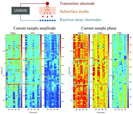
Firstly, the system design description of UMMAI system for well logging is given. UMMAI mainly consists of a transmitter unit, 6 signal acquisition pads and a control-processing unit. A stratigraphic simulation system is also built for UMMAI test convenience, which can simulate the variation of the stratigraphic impedance. The schematic architecture of UMMAI is shown in
Figure 3. As shown in
Figure 3, the control-processing unit and transmitter unit are located in the heat resistant cylinder case of the instrument, the acquisition units are located in the retractable pad plates. The pictures of control-processing unit, transmitter unit and signal acquisition unit in UMMAI are shown in
Figure 4.
The system can works in three modes: operative mode, calibration mode, and self-checking mode. In operative mode, the UMMAI system is placed into a real well environment and the variable current amplitude and phase caused by the external mud and stratum is collected when the UMMAI moves along the well direction. In calibration mode, the stratigraphic simulation system is used instead of the real well environment, which can simulate the variable impedance environment via a known resistor array under the control of control-processing unit. In self-checking mode, the sine signals are directly looped into the control-processing unit, and the working state of the transmitter unit can be judged.
In the control-processing unit, a FPGA is selected as the master control device owning to its outstanding performance in wide operation temperature range, flexible programming characteristic and economical price. A DDS device is used as the waveform generator to produce high-resolution low-distortion sine signals ranging from 100 Hz to 20 MHz under the control of FPGA. Due to the insufficient driving power of control-processing unit, an transmitter unit with output power self detection function is designed to increase the driving ability. The produced signals are amplified in transmitter unit and sent to the transmitter electrode, either to drive the subsurface media or for self-checking purpose. The signal transmission line to transmitter electrode is wrapped on the magnetic ring to suppress the electromagnetic interference introduced by the multi-channel high–frequency signal transmission and working environment. In addition, the transmitting unit is also equipped with a self-check circuit to improve the efficiency of the circuit fault self-check.
The sine signals pass through the actual subsurface media or the stratigraphic simulation system, and received by the receiver array electrodes on 6 signal acquisition pads. The detection front-end of the data acquisition circuit first uses a negative feedback operational amplifier to convert the weak current signal to voltage signal for the subsequent signal amplification and filtering operations. The signals are processed in differential mode for the consideration of the common-mode signal rejection. Then the differential output signal of the data acquisition unit is sent to the control-processing unit, where the signal amplitude and phase are sampled by a logarithmic-amplifier-based ADC with a high dynamic range.
There are a front-end sampling circuit, a reconfigurable operational amplifier, a filter circuit and a difference transformation circuit on the control-processing unit. The signals from all data acquisition units are firstly amplified by the reconfigurable amplifier, the cut-off frequency and gain can be flexible configured by FPGA according to the frequency of transmitted signal and environment. In the previous tests, it was found that the amplified signals were greatly disturbed by the noise in the measurement environment, which affected the measurement results to some extent. After adding the post-stage filter circuit, the influence of noise is suppressed greatly and the signal-to-noise ratio is improved. The filtered signals are then sampled in time division multiplexing mode using a multi-channel multiple selection switch and converted into digital samples. The sampled data are framed and transmitted to the surface equipment via FPGA.
In order to achieve high precision and high reliability, the self-checking working mode is added in the UMMAI design. The multi-channel multiple selection switch can be selected to a known input channel, and the amplitude and phase of the channel current can be measured in real time, so the error caused by the non-ideal characteristics such as temperature drift can be evaluated and eliminated.
3.2. Lab Experiment
The formation impedance to be measured commonly varies widely from several hundred ohms to mega ohms. Therefore, the designed UMMAI system is required to have excellent sensitivity, good linearity, high reliability and large dynamic range to adapt to the changes of the subsurface environment.
Firstly, the linearity of UMMAI system output is verified. UMMAI works in the self-checking working mode and three sine excitation signals with frequencies of 100 kHz, 1 MHz and 10 MHz are used. The excitation signal is divided into two signals: the first signal is sent to the transmitter electrode, the second signal is used as the reference signal in sample amplitude and phase calculation. The amplitudes and phases of samples under different signal frequencies, chain gains, transmitter phase shifts and transmitter attenuations are collected and displayed in
Figure 5 and
Figure 6, in which G stands for the gain of receiving chain and P represents the phase of transmitted signal.
As shown in
Figure 5a,b, the normalized sample amplitudes remains almost unchanged when the phase of transmitted signal changes between 0° and 90°, no matter whatever excitation signal frequency and chain gain are used. When the excitation signal frequency increases to 10 MHz and the chain gain is set as 30 dB in
Figure 5c, the differences of normalized sample amplitudes between different transmitted signal phase increases to 1.7 dB, which can be ignored in the following impedance analysis. The results show that the amplitudes of collected samples are immune to the phase of transmitted signal.
Moreover, the results in
Figure 5a show the UMMAI receiver chain can achieve a linear dynamic range no less than 50 dB when the chain gain is set as 15 dB. When the transmitter attenuation is larger than 35 dB, the linear of receiver chain at G = 0 dB is deteriorated due to the low signal-to-noise ratio. The linear of receiver chain at G = 30 dB is also deteriorated when transmitter attenuation is less than 20 dB, which is caused by the nonlinear saturation of the receiver chain. Similar phenomenons happen when the excitation signal frequencies are 1 MHz and 10 MHz, as shown in
Figure 5b,c, despite the nonlinearity degrees of receiver chain are different.
In
Figure 6a, the sample phase changes with the transmitter attenuation obviously when the transmitter attenuation is larger than 30 dB, especially when the receiver chain gain is set as G = 0 dB. This is mainly caused by the low signal-to-noise ratio at the receiver electrode. When the receiver chain gain increases to 15 dB and 30 dB, the differences between sample phase decrease to 5° and 3° while the transmitter attenuation is 50 dB and phase of transmitted signal is 90°. Similar phenomenons happen when the excitation signal frequency is 1 MHz, as shown in
Figure 6b. The linearity of sample phase gives the worst performance when the excitation signal frequency increases to 10 MHz because of the influence of high frequency parasitic components in transmitter and receiver chains on phase.
Next, the capability of linear resistance measurement of UMMAI system is verified. UMMAI works in the operative mode and four sine excitation signals with frequencies of 1 kHz, 10 kHz, 100 kHz and 1 MHz are used. Dozens of resistors with accurate resistances are used for evaluation. The amplitudes and phases of samples under different signal frequencies, chain gains and resistances are collected and displayed in
Figure 7, in which G stands for the gain of receiving chain.
As shown in
Figure 7a, the receiver chain can remain a linear dynamic range larger than 40 dB at G = 20 dB when measuring the resistances from 1 kΩ to 200 kΩ. By selecting receiver gain reasonably and combining the samples at different gains, UMMAI can cover a linear resistance measurement range from 100 Ω to 2 MΩ using 1 kHz excitation signal.
Figure 7b validates the similar linear resistance measurement ability of UMMAI when using 10kHz excitation signal. In
Figure 7c, the linear resistance measurement range of UMMAI narrows to some extent due to poor high frequency response, which is from 100 Ω to 467.2 kΩ. The linear performance continues to deteriorate using 1 MHz excitation signal, while the linear resistance measurement range is from 100 Ω to 100 kΩ.
Finally, the accurate performance of UMMAI resistance measurement is evaluated. UMMAI works in the operative mode and three sine excitation signals with frequencies of 100 kHz, 1 MHz and 10 MHz are used. Dozens of resistors with accurate resistances are used for evaluation. The measured resistance values of resistors and phases of samples under different signal frequencies, chain gains and resistances are collected and displayed in
Figure 8 and
Figure 9, in which G stands for the gain of receiving chain.
As shown in
Figure 8a, UMMAI can cover a linear resistance measurement range from 2 kΩ to 10 MΩ using 100 kHz excitation signal by selecting receiver gain reasonably and combining the samples at different gains, which is also the same using 1-MHz excitation signal in
Figure 8b. The linearity of UMMAI reduces in
Figure 8c, while the linear resistance measurement range is from 2 kΩ to 100 kΩ when using 10 MHz excitation signal. The results in
Figure 9 show that the difference in sample phase is less than 5° when the receiver chain of UMMAI achieves a good resistance measurement linearity, however, the sample phase consistency will deteriorate badly in non-linear resistance measurement range, especially when using high frequency excitation signal.
3.3. Field Test
In this section, the array imaging performance of UMMAI is evaluated in three different field tests. In each field test, UMMAI is placed into a simulated borehole, the wall of which is engraved with various patterns, as is shown in
Figure 10. UMMAI works in the operative mode and three sine excitation signals with frequencies of 200 kHz, 1 MHz and 5 MHz are used.
In the first test, the simulated borehole is filled with oil-based mud. UMMAI moves from 8.4 to 11.1 m in depth and collects the resistance samples from 15 receiver electrodes on 6 pads, as shown in
Figure 3.
After the samples are collected, the samples from different electrodes on the same pad are aligned first to eliminate the depth differences between electrodes. Then the samples from different pads are aligned to eliminate the depth differences between pads. After the alignment processing is finished, the background signal in the samples is removed through an average filter, and the modulus and phases of filtered samples are used for imaging.
The errors associated to the resistivity measurements during the field experiment are mainly caused by depth differences between electrodes, depth differences between pads and filter artifacts. The depth differences are eliminated in the alignment processing and the influence of filter artifacts can be suppressed to acceptable level by optimizing filter parameters. The modulus and phases of filtered samples are illustrated in
Figure 11 and
Figure 12.
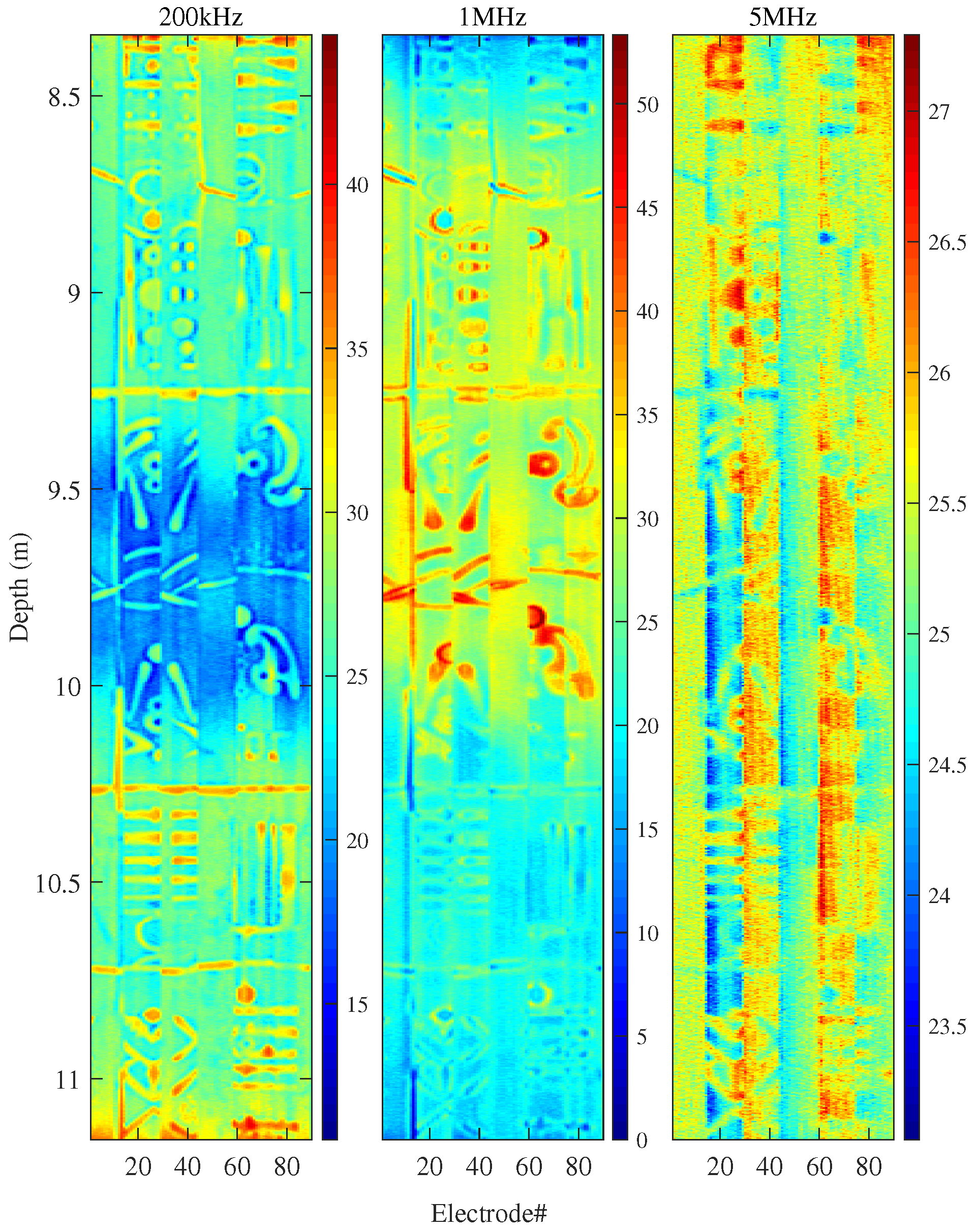
As shown in
Figure 11, the patterns on the borehole wall can be imaged clearly with 200 kHz excitation signal in oil-based mud environment. At the depth of 9.13 m, a horizontal notch with a width of 8 mm can be distinguished. The amplitude of samples ranges from 0 to 322. The results with 1 MHz excitation signal gives slightly worse image of patterns, with the amplitude of samples ranging from 48 to 246, the scope of which is smaller than that of 200 kHz. It is considered to be caused by the high frequency attenuation in receiver channels and the influence of filling mud, which reduces the signal-to-noise ratio at the receiver electrodes. When the excitation frequency increases to 5 MHz, this phenomenon becomes more obvious and the pattern image is unable to provide any information about the borehole wall, since the sample amplitude ranges from 88 to 89.
As shown in
Figure 12, the patterns on the borehole wall can also be imaged clearly using sample phases with 200 kHz and 1 MHz excitation signals, which agrees well with the results in
Figure 11. The pattern image using sample phases with 5 MHz in
Figure 12 performs better than that in
Figure 11, in which several patterns can be distinguished.
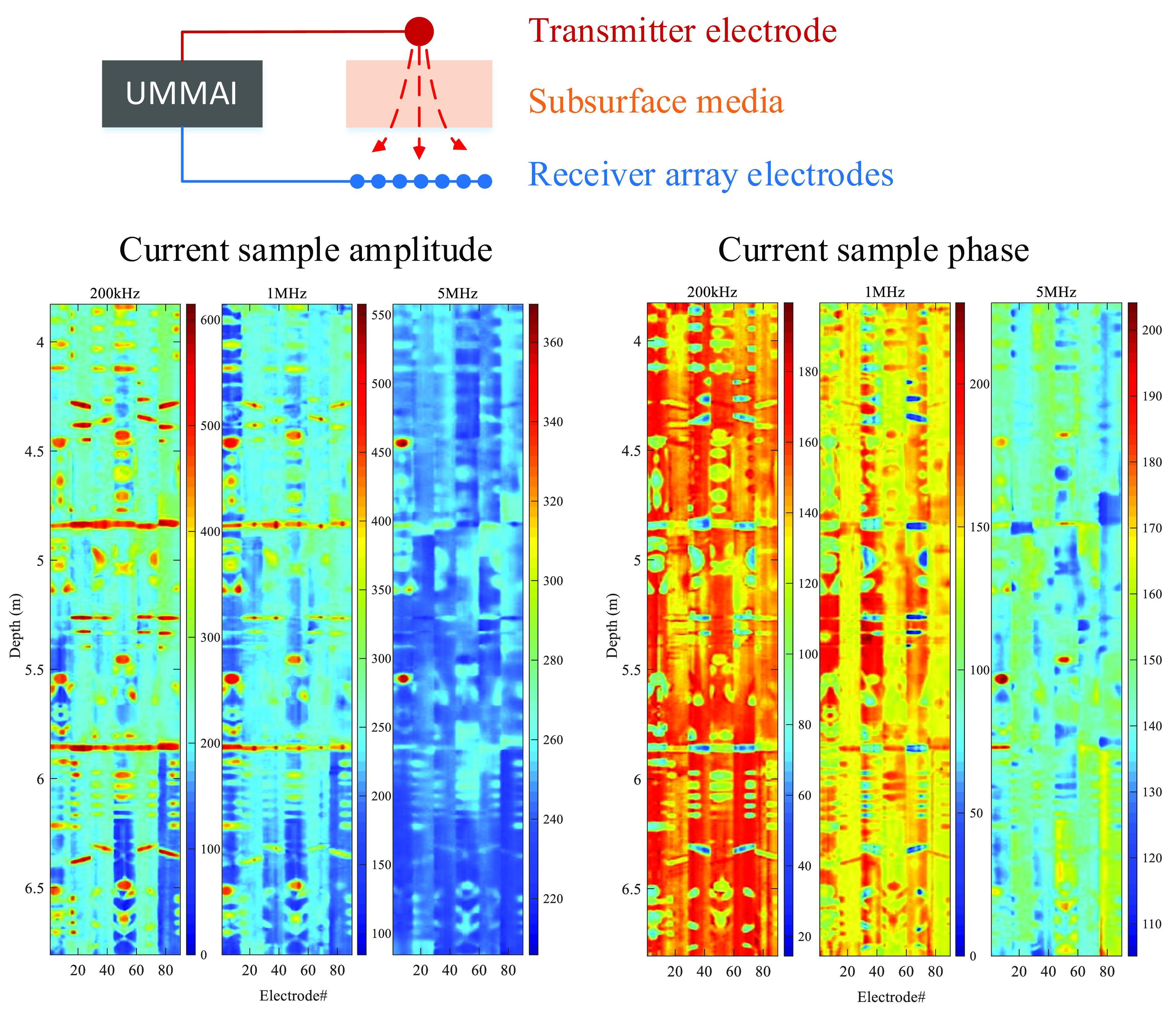
In the second test, the simulated borehole is filled with water-based mud. UMMAI moves from 3.8 m to 6.8 m. The align operations and average filter are also applied over the samples. The modulus and phases of filtered samples are illustrated in
Figure 13 and
Figure 14.
As shown in
Figure 13, the patterns on the borehole wall can be imaged clearly with 200 kHz and 1 MHz excitation signals in water-based mud environment. At the depth ranging from 5.27 to 5.4 m, three horizontal notch with a width of 10 mm can be distinguished. Owing to the lower resistivity of water than oil, the amplitude of samples in 200 kHz and 1 MHz ranges from 0 to 614, and from 84 to 558, respectively, which are larger than those in
Figure 11. Although the results with 5 MHz excitation signal still has the worst performance in
Figure 13, it behaves better than that in
Figure 11, since more pattern details with 5 MHz excitation signal in
Figure 13 are revealed, especially at depths from 5.8 m to 6.8 m. The sample amplitude with 5 MHz ranges from 205 to 369. The images in
Figure 14 demonstrates consistent results with those in
Figure 13.
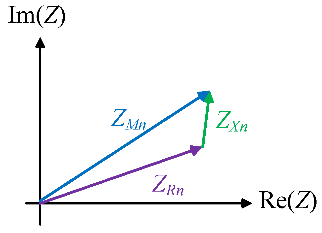
Since the stratum impedance is frequency dependent, the sample amplitude will change in different magnetic fields. Moreover, the gap mud impedance between receiver electrode and stratum, , will also change in different environments, which will introduce changes in the measured impedance . The increase of working frequency leads to increase in the stratum impedance and gap mud impedance, which will reduce the current flowing the sample resistor and decrease the sample amplitudes. The reduced signal-to-noise ratio in higher working frequency environment will influence the imaging quality.
In the third test, the simulated borehole is filled with water-oil mixed mud. UMMAI moves from 10.9 m to 12 m. The same align operations and average filter are applied over the samples. The modulus and phases of filtered samples are illustrated in
Figure 15 and
Figure 16.
As shown in
Figure 15, the patterns on the borehole wall can also be imaged clearly with 200 kHz and 1 MHz excitation signals in water-oil mixed mud environment. At the depth ranging from 11.4 m to 11.6 m, four horizontal notches with a width of 8 mm can be distinguished. The amplitude of samples in 200 kHz and 1 MHz ranges from 0 to 398, and from 126 to 214, respectively, which are larger than those in
Figure 11 and smaller than those in
Figure 13. The results with 5 MHz excitation signal also gives acceptable image of patterns. The sample amplitude with 5 MHz ranges from 136 to 201. The images in
Figure 16 demonstrates consistent results with those in
Figure 15.
Since the UMMAI system is a multi–frequency working system, the resolution performance of UMMAI is comprehensively evaluated with amplitude and phase images with all working frequencies. The above results show that UMMAI can provide high resolution images in different mud environments.
According to the public literatures from Baker Hughes [
30] and Halliburton [
31], the vertical and azimuthal resolution of STAR imager is about 0.2 inch (5 mm), and its applicable mud resistivity range is from 0.01 Ω/m to 10 Ω/m, which is not suitable for oil-based mud environment.The resolution of EMI and StrataXaminer is about 0.2 in (5 mm), and they are only applicable in an oil-based mud environment.
In the field tests of UMMAI, limited to the minimum notch width in the test fields, several horizontal notches with a width of 8 mm can be distinguished in
Figure 11 and
Figure 15. Therefore, UMMAI is regared to own a resolution better than 8 mm and has comparable imaging performance with mainstream commercial logging equipments, which is suitable and universal in multiple mud environments.


