
Fine-Grained Ship Classification by Combining CNN and Swin Transformer

Abstract
:
1. Introduction
2. Models
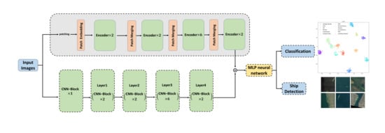
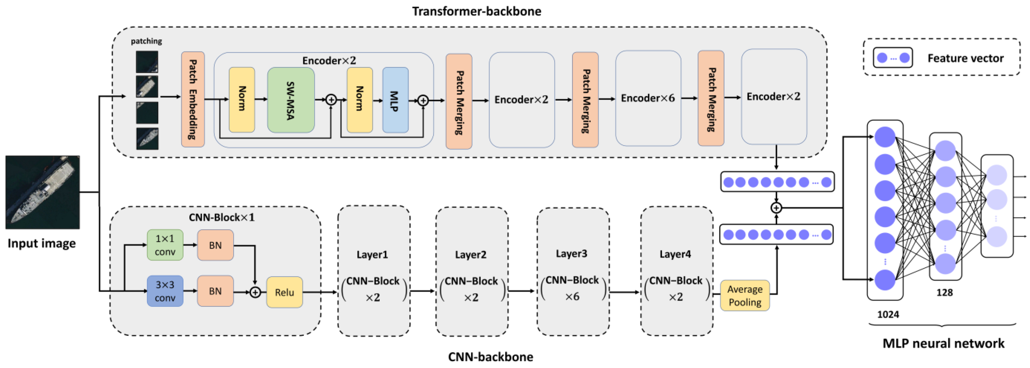
2.1. Overview
2.2. Convolutional Neural Network (CNN) Backbone
2.2.1. Layers
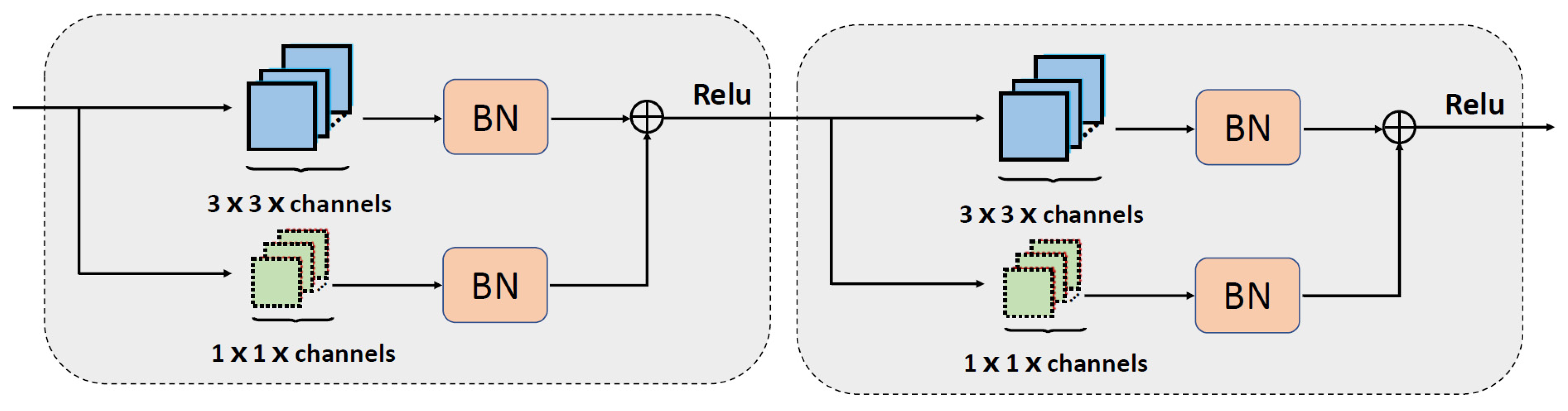
2.2.2. CNN-Block
2.3. Transformer Backbone
2.3.1. Patch Embedding
2.3.2. Encoder
2.4. Multi-Layer Perceptron (MLP) Neural Network
3. Experiment
3.1. Datasets
3.1.1. FGSC-23 Dataset
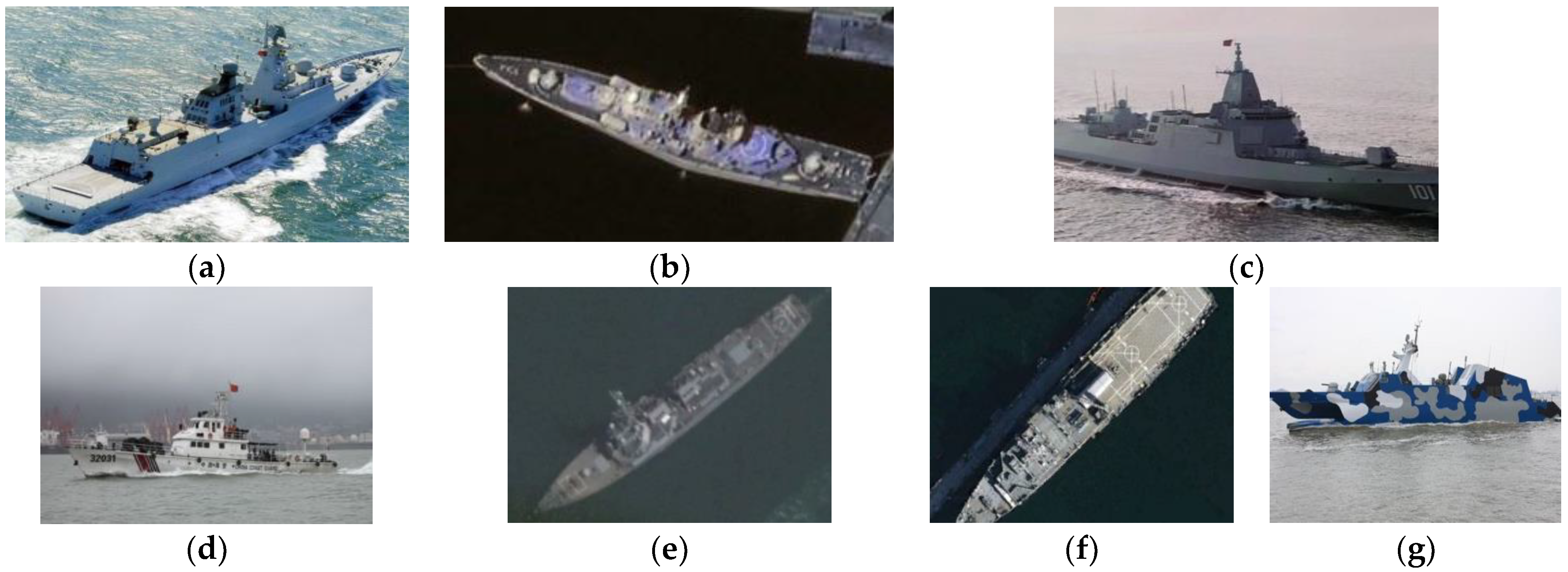
3.1.2. Military Ship Dataset
3.1.3. HRSC2016
3.1.4. FAIR1M
3.2. Experiments and Results
3.2.1. Experiment Details and Basic Results of CNN-Swin Model
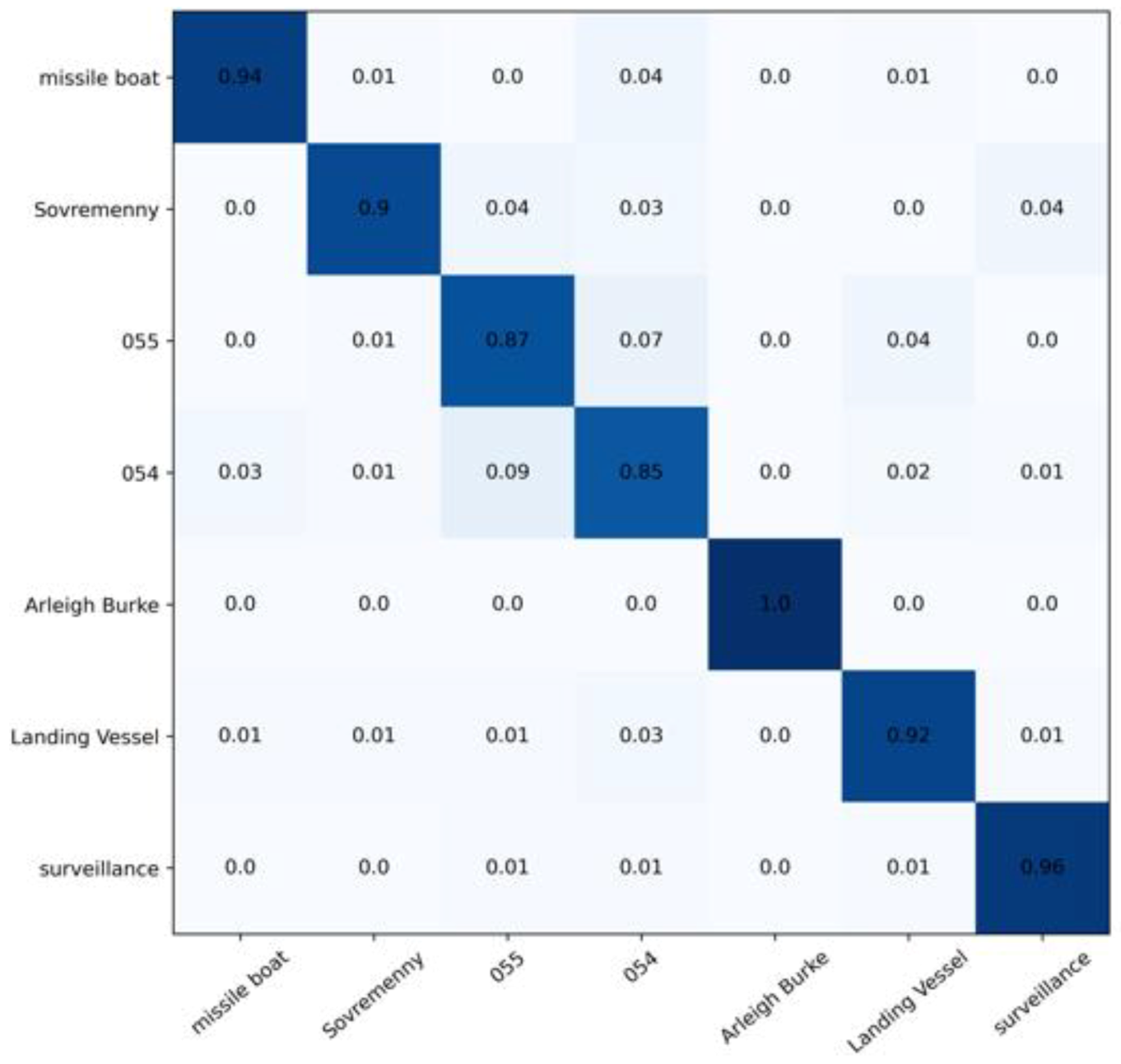
- The model was trained well overall. The Arleigh Burke class destroyers had the highest accuracy of 100%. The missile boat, landing vessel, and surveillance boat had accuracies higher than 90%. In general, the model had a high classification accuracy for the seven categories of ship image, demonstrating the reliability and robustness of the model with ship images as the objects;
- Type-055 destroyers and Type-054 frigates had poor classification results, with accuracy rates of 0.87% and 0.85%, respectively, where 9% of Type-054 frigates were misclassified as Type-055 destroyers by the model, and 7% of Type-055 destroyers were misclassified as Type-054 frigates by the model. The reason was that the two are extremely similar in hull structure and overall superstructure, differing only partially in the superstructures. Specifically, in addition to the main bridge, the Type-055 destroyer has an integrated mast that is nearly the same height as the main bridge; the Type-054 frigate has a lower mast arranged at the rear and a radar with a spherical outer cover on top. In addition, the stern of the Type-054 frigate has a helicopter hangar, while the Type-055 destroyer does not, which results in some subtle differences in the superstructures at the stern. Compared to the more evident, fine-grained features, such as the superstructures in the other categories, the fine-grained feature differences between Type-055 destroyers and Type-054 frigates are not significant enough to give rise to a 7–9% classification error rate.
3.2.2. Performance Comparison for Image Classification
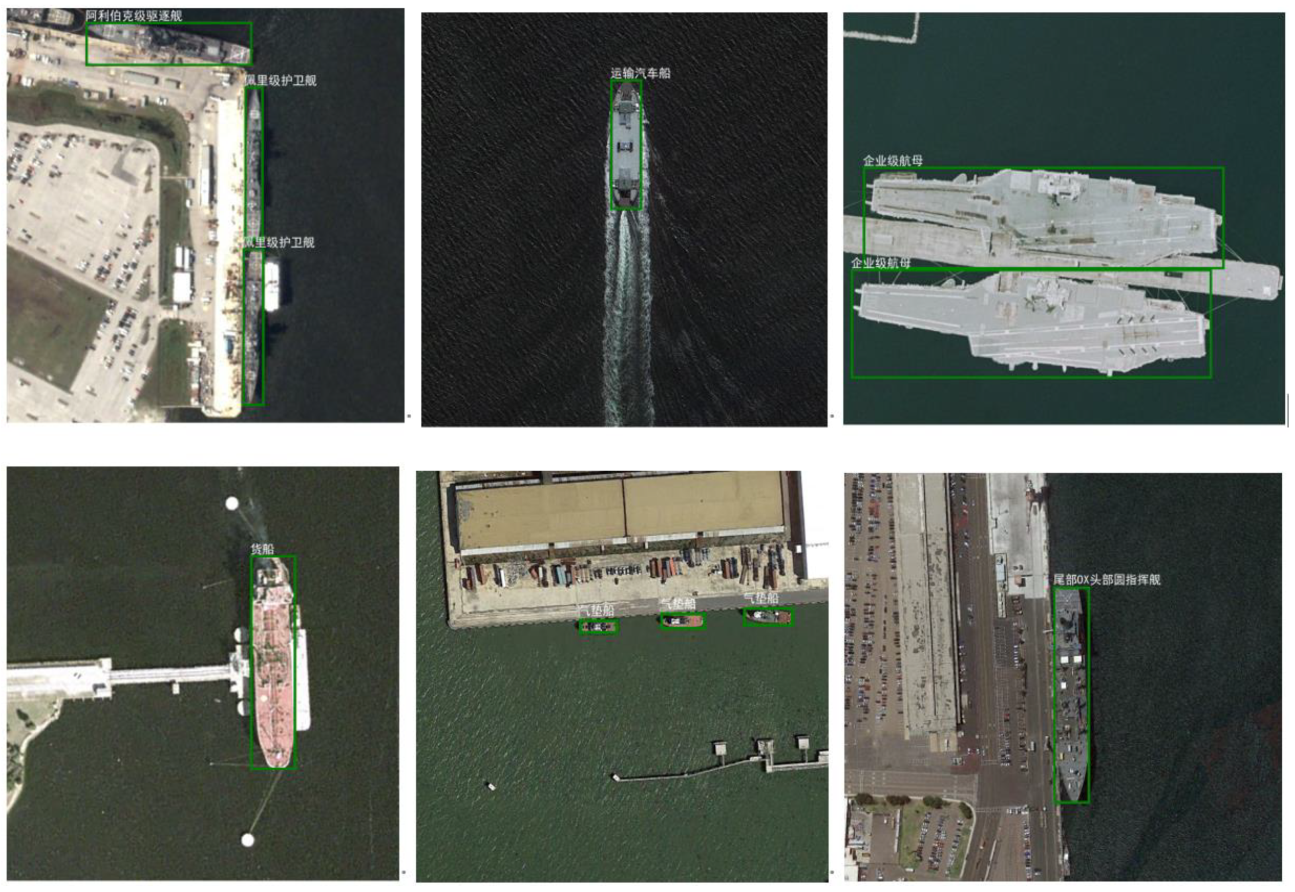
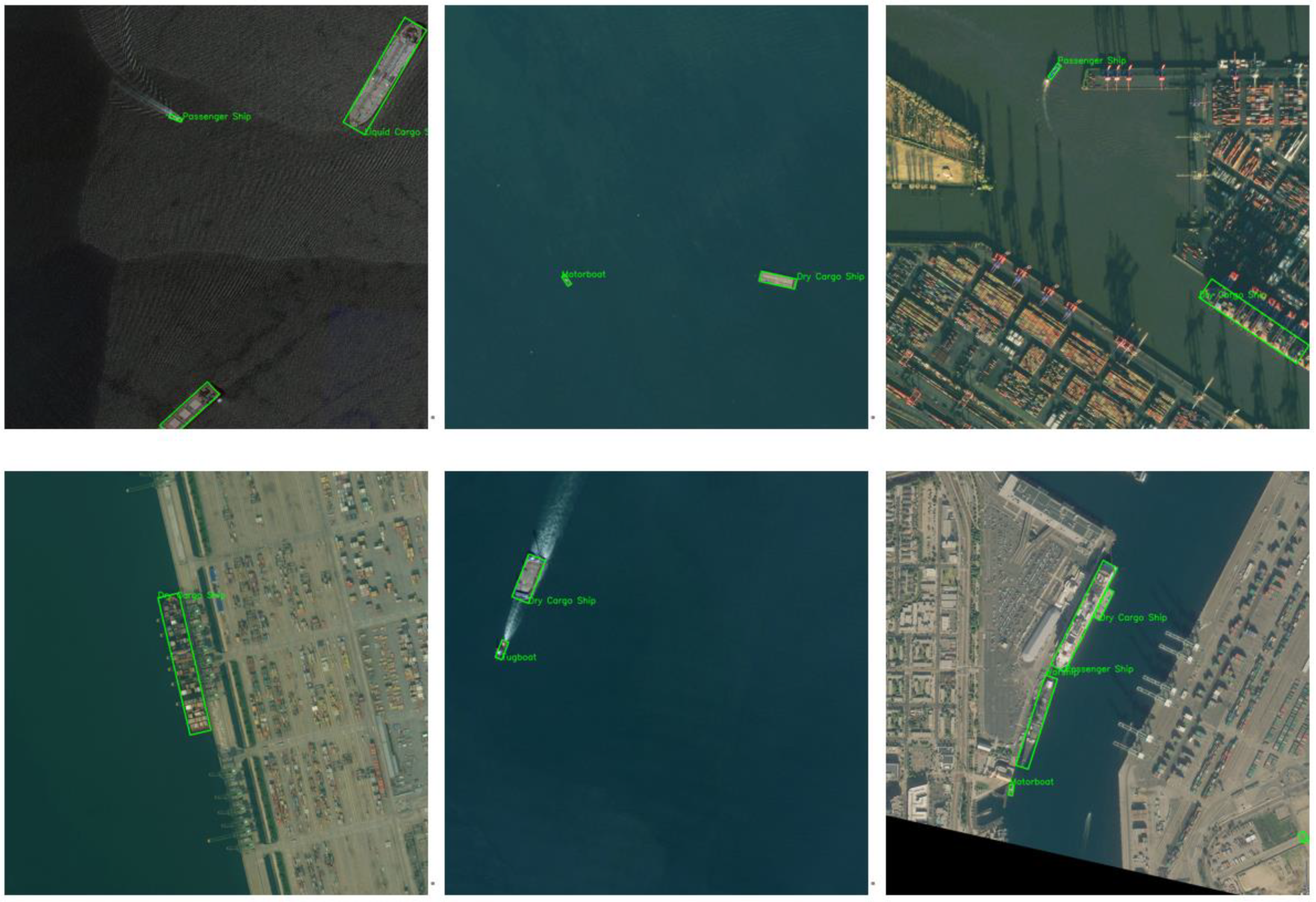
3.2.3. Performance Comparison for Ship Detection
3.2.4. Ablation Studies
4. Conclusions
Author Contributions
Funding
Data Availability Statement
Conflicts of Interest
References
- Krizhevsky, A.; Sutskeve, I.; Hinton, G.E. Imagenet classification with deep convolutional neural networks. In Proceedings of the Advances in neural information processing systems, Lake Tahoe, NV, USA, 3–6 December 2012; pp. 1097–1105. [Google Scholar]
- Simonyan, K.; Zisserman, A. Very deep convolutional networks for large-scale image recognition. In Proceedings of the International Conference on Learning Representations, San Diego, CA, USA, 7–9 May 2015. [Google Scholar]
- Szegedy, C.; Liu, W.; Jia, Y.; Sermanet, P.; Reed, S.; Anguelov, D.; Erhan, D.; Vanhoucke, V.; Rabinovich, A. Going deeper with convolutions. In Proceedings of the IEEE Conference on Computer Vision and Pattern Recognition, Boston, MA, USA, 8–10 June 2015; pp. 1–9. [Google Scholar]
- Ioffe, S.; Szegedy, C. Batch normalization: Accelerating deep network training by reducing internal covariate shift. In Proceedings of the International Conference on Machine Learning, Lille, France, 6–11 July 2015. [Google Scholar]
- Szegedy, C.; Vanhoucke, V.; Ioffe, S.; Shlens, S.; Wojna, Z. Rethinking the inception architecture for computer vision. In Proceedings of the IEEE Conference on Computer Vision and Pattern Recognition, Las Vegas, NV, USA, 27–30 June 2016. [Google Scholar]
- Szegedy, C.; Ioffe, S.; Vanhoucke, V.; Alemi, A. Inception-v4, inception-resnet and the impact of residual connections on learning. In Proceedings of the AAAI Conference on Artificial Intelligence, Hilton San Francisco, CA, USA, 4–9 February 2017. [Google Scholar]
- He, K.; Zhang, X.; Ren, S.; Sun, J. Deep residual learning for image recognition. In Proceedings of the IEEE Conference on Computer Vision and Pattern Recognition, Las Vegas, NV, USA, 27–30 June 2016; pp. 770–778. [Google Scholar]
- Huang, G.; Liu, Z.; Maaten, L.V.D.; Weinberger, K.Q. Densely connected convolutional net- works. In Proceedings of the IEEE conference on computer vision and pattern recognition, Honolulu, HI, USA, 21–26 July 2017; pp. 4700–4708. [Google Scholar]
- Howard, A.G.; Zhu, M.; Chen, B.; Kalenichenko, D.; Wang, W.; Weyand, T.; Andreetto, M.; Adam, H. Mobilenets: Efficient convolutional neural networks for mobile vision applications. arXiv 2017, arXiv:1704.04861. [Google Scholar]
- Sandler, M.; Howard, A.G.; Zhu, M.; Zhmoginov, A.; Chen, L. Mobilenetv2: Inverted residuals and linear bottlenecks. In Proceedings of the IEEE/CVF Conference on Computer Vision and Pattern Recognition, Salt Lake City, UT, USA, 18–23 June 2018. [Google Scholar]
- Howard, A.; Sandler, M.; Chu, G.; Chen, L.; Chen, B.; Tan, M.; Wang, W.; Zhu, Y.; Pang, R.; Vasudevan, V. Searching for mobilenetv3. In Proceedings of the IEEE/CVF International Conference on Computer Vision, Seoul, Korea, 27 October–2 November 2019. [Google Scholar]
- Tan, M.; Le, Q. Efficientnet: Rethinking model scaling for convolutional neural networks. In Proceedings of the International Conference on Machine Learning, Long Beach, CA, USA, 9–16 June 2019. [Google Scholar]
- Lin, T.; Dollar, P.; Girshick, R.; He, K.; Hariharan, B.; Belongie, S. Feature pyramid networks for object detection. In Proceedings of the IEEE Conference on Computer Vision and Pattern Recognition, Honolulu, HI, USA, 21–26 July 2017; pp. 936–944. [Google Scholar]
- Jeon, H.; Yang, C. Enhancement of Ship Type Classification from a Combination of CNN and KNN. Electronics 2021, 10, 1169. [Google Scholar] [CrossRef]
- Li, J.; Ruan, J.; Xie, Y. Research on the Development of Object Detection Algorithm in the Field of Ship Target Recognition. Int. Core J. Eng. 2021, 7, 233–241. [Google Scholar]
- Julianto, E.; Khumaidi, A.; Priyonggo, P.; Munadhif, I. Object recognition on patrol ship using image processing and convolutional neural network (CNN). J. Phys. Conf. Ser. 2020, 1450, 012081. [Google Scholar] [CrossRef] [Green Version]
- Chen, Z.; Chen, D.; Zhang, Y.; Cheng, X.; Zhang, M.; Wu, C. Deep learning for autonomous ship-oriented small ship detection. Saf. Sci. 2020, 130, 104812. [Google Scholar] [CrossRef]
- Zhao, S.; Xu, Y.; Li, W.; Lang, H. Optical Remote Sensing Ship Image Classification Based on Deep Feature Combined Distance Metric Learning. J. Coast. Res. 2020, 102, 82–87. [Google Scholar] [CrossRef]
- Xu, C.; Yin, C.; Wang, D.; Han, W. Fast ship detection combining visual saliency and a cascade CNN in SAR images. IET Radar Sonar Navig. 2020, 14, 1879–1887. [Google Scholar] [CrossRef]
- Gao, X. Design and Implementation of Marine Automatic Target Recognition System Based on Visible Remote Sensing Images. J. Coast. Res. 2020, 115, 277–279. [Google Scholar] [CrossRef]
- Ren, Y.; Yang, J.; Zhang, Q.; Guo, Z. Multi-Feature Fusion with Convolutional Neural Network for Ship Classification in Optical Images. Appl. Sci. 2019, 20, 4209. [Google Scholar] [CrossRef] [Green Version]
- Li, Z.; Zhao, B.; Tang, L.; Li, Z.; Feng, F. Ship classification based on convolutional neural networks. J. Eng. 2019, 21, 7343–7346. [Google Scholar]
- Bi, F.; Hou, J.; Chen, L.; Yang, Z.; Wang, Y. Ship Detection for Optical Remote Sensing Images Based on Visual Attention Enhanced Network. Sensors 2019, 10, 2271. [Google Scholar] [CrossRef] [PubMed] [Green Version]
- Vaswani, A.; Shazeer, N.; Parmar, N.; Uszkoreit, J.; Jones, L.; Gomez, A.N.; Kaiser, L.; Polosukhin, I. Attention is all you need. In Proceedings of the Advances in Neural Information Processing Systems, Long Beach, CA, USA, 4–9 December 2017; pp. 5998–6008. [Google Scholar]
- Dosovitskiy, A.; Beyer, L.; Kolesnikov, A.; Weissenborn, D.; Zhai, X.; Unterthiner, T.; Dehghani, M.; Minderer, M.; Heigold, G.; Gelly, S.; et al. An image is worth 16×16 words: Transformers for image recognition at scale. In Proceedings of the International Conference on Learning Representations, Vienna, Australia, 3–7 May 2021. [Google Scholar]
- Touvron, H.; Cord, M.; Douze, M.; Massa, F.; Sablayrolles, A.; Jegou, H. Training data-efficient image transformers & distillation through attention. arXiv 2020, arXiv:2012.12877. [Google Scholar]
- Yuan, L.; Chen, Y.; Wang, T.; Yu, W.; Shi, Y.; Tay, F.E.; Feng, J.; Yan, S. Tokens- to-token vit: Training vision transformers from scratch on imagenet. arXiv 2021, arXiv:2101.11986. [Google Scholar]
- Chu, X.; Zhang, B.; Tian, Z.; Wei, X.; Xia, H. Do we really need explicit position encodings for vision transformers? arXiv 2021, arXiv:2102.10882. [Google Scholar]
- Han, K.; Xiao, A.; Wu, E.; Guo, J.; Xu, C.; Wang, Y. transformer in transformer. arXiv 2021, arXiv:2103.00112. [Google Scholar]
- Wang, W.; Xie, E.; Li, X.; Fan, D.; Song, K.; Liang, D.; Lu, T.; Luo, P.; Shao, L. Pyramid vision transformer: A versatile backbone for dense prediction without convolutions. arXiv 2021, arXiv:2102.12122. [Google Scholar]
- Heo, B.; Yun, S.; Han, D.; Chun, S.; Choe, J.; Oh, S.J. Rethinking Spatial Dimensions of Vision Transformers. arXiv 2021, arXiv:2103.16302v2. [Google Scholar]
- Touvron, H.; Cord, M.; Sablayrolles, A.; Synnaeve, G.; Jégou, H. going deeper with Image Transformers. arXiv 2021, arXiv:2103.17239v2. [Google Scholar]
- Liu, Z.; Lin, Y.; Cao, Y.; Hu, H.; Wei, Y.; Zhang, Z.; Lin, S.; Guo, B. Swin Transformer: Hierarchical Vision Transformer using Shifted Windows. arXiv 2021, arXiv:2103.14030v2. [Google Scholar]
- Xu, X.; Feng, Z.; Cao, C.; Li, M.; Wu, J.; Wu, Z.; Shang, Y.; Ye, S. An Improved Swin Transformer-Based Model for Remote Sensing Object Detection and Instance Segmentation. Remote Sens. 2021, 13, 4779. [Google Scholar] [CrossRef]
- Huang, B.; Guo, Z.; Wu, L.; He, B.; Li, X.; Lin, Y. Pyramid Information Distillation Attention Network for Super-Resolution Reconstruction of Remote Sensing Images. Remote Sens. 2021, 13, 5143. [Google Scholar] [CrossRef]
- Yao, L.; Zhang, X.; Lyu, Y.; Sun, W.; Li, M. FGSC-23: A large-scale dataset of high-resolution optical remote sensing image for deep learning-based fine-grained ship recognition. J. Image Graph. 2021, 26, 2337–2345. [Google Scholar]
- Liu, Z.; Wang, H.; Weng, L.; Yang, Y. Ship rotated bounding box space for ship extraction from high-resolution optical satellite images with complex back- grounds. IEEE Geosci. Remote Sens. Lett. 2016, 13, 1074–1078. [Google Scholar] [CrossRef]
- Sun, X.; Wang, P.; Yan, Z.; Xu, F.; Wang, R.; Diao, W.; Chen, J.; Li, J.; Feng, Y.; Xu, T.; et al. FAIR1M:A Benchmark Dataset for Fine-grained Object Recognition in High-Resolution Remote Sensing Imagery. arXiv 2021, arXiv:2103.05569. [Google Scholar]
- Springenberg, J.T.; Dosovitskiy, A.; Riedmiller, M.A. Striving for Simplicity: The All Convolutional Net. arXiv 2014, arXiv:1412.6806. [Google Scholar]
- Han, D.; Yun, S.; Heo, B.; Yoo, Y. Rethinking channel dimensions for efficient model design. In Proceedings of the IEEE/CVF Conference on Computer Vision and Pattern Recognition, Nashville, TN, USA, 20–25 June 2021; pp. 732–741. [Google Scholar]
- Radosavovic, I.; Kosaraju, R.P.; Girshick, R.; He, K.; Dollar, P. Designing network design spaces. In Proceedings of the IEEE/CVF Conference on Computer Vision and Pattern Recognition, Seattle, WA, USA, 13–19 June 2020; pp. 10428–10436. [Google Scholar]
- Ding, X.; Zhang, X.; Ma, N.; Han, J.; Ding, G.; Sun, J. RepVGG: Making VGG-style convnets great again. In Proceedings of the 2021 IEEE/CVF Conference on Computer Vision and Pattern Recognition (CVPR), Nashville, TN, USA, 20–25 June 2021. [Google Scholar]
- Veit, A.; Wilber, M.J.; Belongie, S. Residual networks behave like ensembles of relatively shallow networks. In Advances in Neural Information Processing Systems, Proceeding of the 30th International Conference on Neural Information Processing Systems, Barcelona, Spain, 5–10 December 2016; Curran Associates Inc.: Red Hook, NY, USA, 2016; pp. 550–558. [Google Scholar]
- Hu, H.; Zhang, Z.; Xie, Z.; Lin, S. Local relation networks for image recognition. In Proceedings of the IEEE/CVF International Conference on Computer Vision (ICCV), Seoul, Korea, 27–28 October 2019; pp. 3464–3473. [Google Scholar]
- Hu, H.; Gu, J.; Zhang, Z.; Dai, J.; Wei, Y. Relation networks for object detection. In Proceedings of the IEEE Conference on Computer Vision and Pattern Recognition, Salt Lake City, UT, USA, 18–23 June 2018; pp. 3588–3597. [Google Scholar]
- Raffel, C.; Shazeer, N.; Roberts, A.; Lee, K.; Narang, S.; Matena, M.; Zhou, Y.; Li, W.; Liu, P.J. Exploring the limits of transfer learning with a unified text-to-text transformer. J. Mach. Learn. Res. 2020, 21, 1–67. [Google Scholar]
- Bao, H.; Dong, L.; Wei, F.; Wang, W.; Yang, N.; Liu, X.; Wang, Y.; Gao, J.; Piao, S.; Zhou, M.; et al. Unilmv2: Pseudo-masked language models for unified language model pre-training. In Proceedings of the International Conference on Machine Learning, Vienna, Austria, 12–18 July 2020; pp. 642–652. [Google Scholar]
- Maaten, L. Accelerating t-SNE using tree-based algorithms. J. Mach. Learn. Res. 2014, 15, 3221–3245. [Google Scholar]
- Xiao, Z.; Qian, L.; Shao, W.; Tan, X.; Wang, K. Axis learning for orientated objects detection in aerial images. Remote Sens. 2020, 12, 908. [Google Scholar] [CrossRef] [Green Version]
- Zhong, B.; Ao, K. Single-stage rotation-decoupled detector for oriented object. Remote Sens. 2020, 12, 3262. [Google Scholar] [CrossRef]
- Ming, Q.; Miao, L.; Zhou, Z.; Song, J.; Yang, X. Sparse Label Assignment for Oriented Object Detection in Aerial Images. Remote Sens. 2021, 13, 2664. [Google Scholar] [CrossRef]
- Everingham, M.; Gool, L.; Williams, C.K.; Winn, J.; Zisserman, A. The Pascal Visual Object Classes (VOC) Challenge. Int. J. Comput. Vis. 2010, 88, 303–338. [Google Scholar] [CrossRef] [Green Version]
- Selvaraju, R.R.; Das, A.; Vedantam, R.; Cogswell, M.; Parikh, D.; Batra, D. Grad-CAM: Visual Explanations from Deep Networks via Gradient-Based Localization. Int. J. Comput. Vis. 2019, 128, 336–359. [Google Scholar] [CrossRef] [Green Version]
- Abnar, S.; Zuidema, W. Quantifying Attention Flow in Transformers. In Proceedings of the 58th Annual Meeting of the Association for Computational Linguistics, Online, 5–10 July 2020; pp. 4190–4197. [Google Scholar]
- Zhu, M.; Hu, G.; Zhou, H.; Wang, S.; Feng, Z.; Yue, S. A Ship Detection Method via Redesigned FCOS in Large-Scale SAR Images. Remote Sens. 2022, 14, 1153. [Google Scholar] [CrossRef]
- Li, L.; Jiang, L.; Zhang, J.; Wang, S.; Chen, F. A Complete YOLO-Based Ship Detection Method for Thermal Infrared Remote Sensing Images under Complex Backgrounds. Remote Sens. 2022, 14, 1534. [Google Scholar] [CrossRef]


| Category of Ships | Number of Images |
|---|---|
| Type-054 frigate | 404 |
| Type-055 destroyer | 409 |
| Sovremenny class destroyer | 420 |
| Surveillance boat | 397 |
| Arleigh Burke class destroyer | 445 |
| Landing vessel | 495 |
| Missile boat | 403 |
| Output Size | CNN Backbone | Transformer Backbone | ||
|---|---|---|---|---|
| CNN-Block | 1 | LN | Patch embeddings | |
| Layer1 | 2 | concat 4 × 4, 128-d, LN | Stage1 | |
| 2 | ||||
| Layer2 | 2 | concat 2 × 2, 256-d, LN | Stage2 | |
| 2 | ||||
| Layer3 | 8 | concat 2 × 2, 512-d, LN | Stage3 | |
| Layer4 | 2 | concat 2 × 2, 1024-d, LN | Stage4 | |
| 2 | ||||
| Average Pooling | ||||
| Fully connected layers | (1024,128), (128, num_class) | |||
| Model | FGSC-32 | Our Military Ship Dataset | ||
|---|---|---|---|---|
| Resolution | Top-1 Accuracy | Resolution | Top-1 Accuracy | |
| Densenet-121 [8] Efficientnet [12] GoogLeNet v4 [6] Resnet-18 [7] VGG-19 [2] Regnet [2020] [40] | 2242 2242 2242 2242 2242 2242 | 84.0% 85.2% 84.2% 81.9% 81.8% 86.1% | 2242 2242 2242 2242 2242 2242 | 76.7% 81.1% 81.6% 84.2% 84.5% 86.4% |
| ViT-tiny [25] ViT-small [25] ViT-base [25] ViT-base [25] CaiT [2020] [32] Swin-tiny [2021] [33] Swin-base [2021] [33] Swin-base [2021] [33] | 2242 2242 2242 3842 2242 2242 2242 3842 | 84.3% 86.3% 87.9% 88.1% 88.0% 86.7% 88.5% 89.1% | 2242 2242 2242 3842 2242 2242 2242 3842 | 81.4% 85.1% 87.2% 87.5% 86.5% 83.4% 88.1% 88.4% |
| CNN-Swin Model | 2242 3842 | 90.9% ± 0.1% 91.4% ± 0.1% | 2242 3842 | 91.9% ± 0.1% 92.1% ± 0.1% |
| Methods | Backbone | Input Size | HRSC2016 mAP(07) |
|---|---|---|---|
| Axis Learning [49] | Resnet101 Resnet50 ViT-S | 800 × 800 800 × 800 384 × 384 | 65.98 64.04 66.72 |
| CNN-Swin | 384 | 67.23 | |
| RRD [50] | Resnet101 VGG16 ViT-S | 768 × 768 384 × 384 384 × 384 | 89.51 84.30 86.79 |
| CNN-Swin | 768 | 90.67 | |
| SLA [51] | Resnet101 Resnet50 ViT-S | 384 × 384 768 × 768 384 × 384 | 87.14 89.51 88.23 |
| CNN-Swin | 384 | 90.56 |
| Methods | Backbone | Input Size | Ship Data of FAIR1M mAP(07) |
|---|---|---|---|
| Axis Learning [49] | Resnet101 Resnet50 ViT-S | 800 × 800 800 × 800 384 × 384 | 33.82 35.72 36.81 |
| CNN-Swin | 384 | 38.52 | |
| RRD [50] | Resnet101 VGG16 ViT-S | 768 × 768 384 × 384 384 × 384 | 36.53 35.64 37.75 |
| CNN-Swin | 768 | 39.77 | |
| SLA [51] | Resnet101 Resnet50 ViT-S | 384 × 384 768 × 768 384 × 384 | 41.94 40.31 42.23 |
| CNN-Swin | 384 | 43.16 |
| Model | AccCNN | AccTran | AccAll |
|---|---|---|---|
| ViT-base Resnet-101 ViT-base + Resnet-101 | — 82.1% 82.1% | 87.2% — 87.2% | 87.2% 81.8% 89.7% |
| CNN-Swin | 83.2% | 88.0% | 91.9% |
| Data Augmentation Methods | Accuracy |
|---|---|
| RandomRotation RandomBrightnessContrast RandomHorizontalFlip ShiftScaleRotate HueSaturationValue RandomResizedCrop | 90.37% 90.59% 91.24% 91.59% 91.72% 91.77% |
| CNN-Swin without data augmentation CNN-Swin+Data Augmentation (Final) | 91.41% 91.94% |
| Model | Batchsize | Computational Time/h | Accuracy |
|---|---|---|---|
| VGG-16 | 8 | 2.38 | 83.9% |
| VGG-19 | 8 | 2.56 | 84.5% |
| CNN-Swin | 8 | 2.66 | 91.9% |
| Swin+VGG-13 Swin+Resnet-50 CNN-Swin | 4 4 4 | 4.86 3.96 3.26 | 89.9% 90.4% 92.0% |
Publisher’s Note: MDPI stays neutral with regard to jurisdictional claims in published maps and institutional affiliations. |
© 2022 by the authors. Licensee MDPI, Basel, Switzerland. This article is an open access article distributed under the terms and conditions of the Creative Commons Attribution (CC BY) license (https://creativecommons.org/licenses/by/4.0/).
Share and Cite
Huang, L.; Wang, F.; Zhang, Y.; Xu, Q. Fine-Grained Ship Classification by Combining CNN and Swin Transformer. Remote Sens. 2022, 14, 3087. https://doi.org/10.3390/rs14133087
Huang L, Wang F, Zhang Y, Xu Q. Fine-Grained Ship Classification by Combining CNN and Swin Transformer. Remote Sensing. 2022; 14(13):3087. https://doi.org/10.3390/rs14133087
Chicago/Turabian StyleHuang, Liang, Fengxiang Wang, Yalun Zhang, and Qingxia Xu. 2022. "Fine-Grained Ship Classification by Combining CNN and Swin Transformer" Remote Sensing 14, no. 13: 3087. https://doi.org/10.3390/rs14133087