Article

A Comparative Analysis of Swarm Intelligence and Evolutionary Algorithms for Feature Selection in SVM-Based Hyperspectral Image Classification

School of Information Engineering, China University of Geosciences (Beijing), 29 Xueyuan Road, Beijing 100083, China
*
Author to whom correspondence should be addressed.
Remote Sens. 2022, 14(13), 3019; https://doi.org/10.3390/rs14133019
Submission received: 20 May 2022 / Revised: 13 June 2022 / Accepted: 21 June 2022 / Published: 23 June 2022

Abstract

:
Feature selection (FS) is vital in hyperspectral image (HSI) classification, it is an NP-hard problem, and Swarm Intelligence and Evolutionary Algorithms (SIEAs) have been proved effective in solving it. However, the high dimensionality of HSIs still leads to the inefficient operation of SIEAs. In addition, many SIEAs exist, but few studies have conducted a comparative analysis of them for HSI FS. Thus, our study has two goals: (1) to propose a new filter–wrapper (F–W) framework that can improve the SIEAs’ performance; and (2) to apply ten SIEAs under the F–W framework (F–W–SIEAs) to optimize the support vector machine (SVM) and compare their performance concerning five aspects, namely the accuracy, the number of selected bands, the convergence rate, and the relative runtime. Based on three HSIs (i.e., Indian Pines, Salinas, and Kennedy Space Center (KSC)), we demonstrate how the proposed framework helps improve these SIEAs’ performances. The five aspects of the ten algorithms are different, but some have similar optimization capacities. On average, the F–W–Genetic Algorithm (F–W–GA) and F–W–Grey Wolf Optimizer (F–W–GWO) have the strongest optimization abilities, while the F–W–GWO requires the least runtime among the ten. The F–W–Marine Predators Algorithm (F–W–MPA) is second only to the two and slightly better than F–W–Differential Evolution (F–W–DE). The F–W–Ant Lion Optimizer (F–W–ALO), F–W–I-Ching Divination Evolutionary Algorithm (F–W–IDEA), and F–W–Whale Optimization Algorithm (F–W–WOA) have the middle optimization abilities, and F–W–IDEA takes the most runtime. Moreover, the F–W–SIEAs outperform other commonly used FS techniques in accuracy overall, especially in complex scenes.

Graphical Abstract

1. Introduction

Recent developments in remote sensing technology have made hyperspectral images (HSIs) more widely available in various fields [1,2,3]. HSI contains hundreds of narrow, continuously arranged spectral bands, and each band represents a one-dimensional feature [4]. The high spectral resolution provides a wealth of information, while yielding the Hughes effect [5], also known as the curse of dimensionality. The Hughes effect occurs because the narrow adjacent bands [6] of HSI result in redundant information ultimately interferes with classification. Therefore, removing redundant bands without reducing classification accuracy [7] is an important and urgent issue. There are two typical data reduction techniques [8]: feature extraction and FS. Feature extraction techniques (e.g., Principal Component Analysis and Linear Discriminant Analysis) are designed to compress data by using mathematical transformations. Due to every band of the HSI having its corresponding image, the way of feature extraction that the high-dimensional feature space is mapped to a low-dimensional space by linear or nonlinear transformation could not keep the primitive physical significance of the HSI [9]. Thus, feature extraction techniques are not suitable for the dimensionality reduction of HSIs, and so FS has been one of the effective means for solving this issue on HSIs [10], specifically by selecting the optimal subset from all the original bands to gain the desired classification performance.
FS algorithms generally contain three categories of models: filter, wrapper, and hybrid models [11]. Filter models mainly use statistical or probabilistic characteristics of the datasets for FS [12]. They are computationally efficient and are suitable for high-dimensional datasets, as they do not require any machine learning (ML) algorithm. In contrast to filter models, wrapper models use a predetermined ML algorithm to calculate the accuracy of the selection [13]. They can achieve higher prediction accuracy. Still, they also have to bear the higher computational cost. Filter models and wrapper models, in other words, are the opposite in terms of advantages and disadvantages [14]. As the combination of filter and wrapper models, hybrid models combine the benefits of both and avoid their weaknesses, thus promising better results. Many recent studies [15,16,17,18] have applied hybrid models for FS on HSIs. For instance, Xie [15] divided the spectral interval by the filter method of information gain and then combined the GWO algorithm with the SVM classifier to form a wrapper model to obtain the best feature subset; Wang [18] first used the correlation coefficient metric to cull the highly relevant bands and then used the wrapper model containing Sine cosine algorithm (SCA) algorithm to perform a refined search. Through the structure of the hybrid models used in the above literature, it is evident that the models can be summarized in a two-step approach [11]. The first step is based on the filter model to select the candidate features from all the bands, and this reduces the number of features. The second step uses the wrapper model to choose the optimal subset from the candidate features. The hybrid models can thus also be called filter–wrapper (F–W) models.
The filter approaches used in the F–W model mainly fall into two categories: (1) employing one of the commonly used filter-based algorithms (e.g., ReliefF) to evaluate a score of each band according to its criterion and selecting the top-ranked bands to construct the feature subset considered in the wrapper model [11,19,20,21]; and (2) dividing all the bands into many spectral subspaces based on the information criteria (e.g., inter-spectral correlation and mutual information), selecting each subspace’s representative bands according to the wrapper model [8,15,22]. The filter model can obtain the candidate features and reduce the search space for the wrapper model, but it cannot find the optimal subset from HSIs. The wrapper model combines a classifier in ML with a wrapper method that utilizes the classifier as a black box to drive the predictive power of the classifier through the wrapper method, thus evaluating the feature subsets. The model is the key to finding the optimal subset. In terms of the classifier, SVM is now the most commonly used supervised classifier, which can efficiently solve classification problems with small sample sizes and high-dimensional datasets. In particular, many studies [10,23,24,25,26] have addressed the HSI classification problem by using SVM and obtained superior classification accuracy. Since the FS problem is an NP-hard problem [16], combining an exhaustive search with a classifier is impractical to evaluate all feature subsets except for small-sized feature spaces. Therefore, most wrapper methods are suboptimal algorithms that search for relatively high-quality subsets with reasonable computational effort. They fall under the following categories [11]: greedy sequential feature selection methods, nested partitioning methods, mathematical programming methods, and metaheuristic methods. In recent years, metaheuristic methods, especially Swarm Intelligence and Evolutionary Algorithms (SIEAs) [27], have been widely applied for their excellent performance [16].
Many studies [10,16,22,28] have used SIEAs in different F–W frameworks for HSI FS. For example, Xie [28] first implemented subspace decomposition by calculating the correlation coefficients between adjacent bands of HSI and then performed the ABC algorithm for FS. Singh [22] applied a similar framework—first segmented the spectral space of HSI into several spectral regions, using a cluster algorithm, and then applied the GA to each subregion to find the optimal subset and finally integrated them. These studies first performed band subspace decomposition and then applied SIEA to search for subsets, which relies too much on the researchers’ prior knowledge [29]. There are also studies that can perform HSI FS without relying on a priori knowledge. For instance, Zhang [16] used maximizing representativeness and minimizing redundancy (mRMR) to obtain representative subsets initially and then performed an exact search, employing the immune clone selection (ICS) algorithm. Moreover, Wang [10] first used the correlation coefficient to remove the highly relevant bands and then used a modified ALO (MALO) and wavelet SVM (WSVM) to reduce the dimensionality of HSIs. Using existing filter methods to obtain the candidate feature subset is convenient, as there is no need for prior knowledge. However, it has been confirmed [12] that using a single filter method on different datasets to select candidate feature subsets is not robust. Given the flaws in these frameworks, this paper aims to use multiple filter-based methods to form an integrated filter model for selecting the informative candidate features in a novel way. Specifically, we merge the bands selected by different filter methods as candidate features. This integrated model can theoretically address these drawbacks and maximize the performance of the SIEAs.
Up to now, there have been many different SIEAs applied to the FS problems [30]. Some are historical but practical for HSIs, such as GA [8], DE [17], Particle Swarm Optimisation (PSO) [31], etc. In addition, others are just emerging for real-world problems other than HSI classification. For instance, Chen et al. [32] proposed the IDEA inspired by Chinese I-Ching in 2016, and it achieved better performance in the benchmark functions. Heidari et al. [33] simulated Harris Hawks Optimizer (HHO) based on the predatory behavior of Harris’s hawk in 2019. Afshin et al. [34] also proposed MPA according to the predatory behavior of marine organisms in 2020 and verified its superior performance in the engineering functions. The evidence reviewed here suggests that scholars have proposed many SIEAs, but few studies have compared the optimization performance of these algorithms for the FS problem, particularly for HSI classification.
To sum up, this paper has two research objectives: (1) to build a hybrid F–W framework that can strike a good balance between the filter component’s efficiency and the wrapper component’s accuracy; and (2) to compare different SIEAs’ performance on HSI FS. To achieve the objectives, we developed a novel F–W framework that integrates several commonly used filter methods in the filter component and applies different SIEAs for comparison in the wrapper component. To demonstrate the framework’s validity, we evaluated and compared the performance of each SIEA under the F–W framework (i.e., F–W–SIEA) with each pure SIEA wrapper on the HSIs. The comparison aspects relate to classification accuracy, the number of selected bands, convergence rate, and relative runtime. Specifically, this paper investigates the following points: (1) comparisons of each F–W–SIEA with the corresponding pure SIEA wrapper; (2) comparisons of different F–W–SIEAs; and (3) comparisons of several representative F–W–SIEAs with commonly used FS techniques, as well as classification with full bands (FBs).

2. Methods

This proposed novel F–W framework has two main components: a filter component, which uses several commonly used filter methods; and a wrapper component, which combines different SIEAs separately to perform comparisons. The filter component uses multiple filter-based methods to rank the bands according to their evaluation scores, selects and unions the top-ranked features obtained from each filter method, and finally generates the candidate features passed to the wrapper component. The wrapper component uses SVM as the classifier, applying different F–W–SIEAs for comparison. The flowchart is shown in Figure 1, and the corresponding details are presented in Section 2.1, Section 2.2, Section 2.3 and Section 2.4.
The standard process for optimizing SVM classification based on each SIEA is shown in Figure 2. Every SIEA follows this process when combined with SVM. First, we generate the initial population and set the corresponding SIEA parameters. Meanwhile, we divide the HSI’s samples into the training and testing set. Second, we train the SVM classifier by combining the training set and each individual containing information on the selected bands and the SVM parameters. Then we evaluate the fitness of each individual in the population. If the stopping criterion is satisfied, we use the information of the best individual to train the optimal SVM classifier and classify all testing image pixels to obtain the result of this SIEA. Moreover, if it is not satisfied, we update the population according to the SIEA rules and repeat the above steps to evaluate the individual fitness and determine whether the stopping criterion is satisfied until the criterion is satisfied.

2.1. The Filter Component of the Framework

Many filter-based methods are currently available for the FS problems. However, the previous research [12] confirmed that no filter method outperforms all other methods, so a single filter-based method may not be robust in different datasets. Therefore, choosing a corresponding appropriate filter algorithm for different datasets can be computationally costly. Based on the situations, the filter component integrates several commonly used filter methods to reduce the uncertainty of a single filter method and make the component more robust. In other words, this filter component utilizes the brainstorms of different filter methods to select a more reliable candidate feature subset than a single filter method.
To ensure the component selects all the valuable bands, we use seven filter algorithms with good performance and operate on different mechanisms. The algorithms include Mutual Information Feature Selection (MIFS) [35], Joint Mutual Information (JMI) [36], Conditional Mutual Information Maximization (CMIM) [37], mRMR [38], Interaction Capping (ICAP) [39], Conditional Infomax Feature Extraction (CIFE) [40], and ReliefF [41]. Specifically, at first, we sort the features by using each algorithm, select the top-ranked features of each, and finally use the union operator to combine all the algorithms’ top-ranked features. In our pre-experimentation, we selected and integrated the top 5–35% (set the interval to 5%) of each algorithm’s sorting features as the candidate feature sets and input these candidate feature sets of different sizes into the wrapper model, respectively. We find that it is appropriate to set the selection and integration of 20% of the top-ranked features of each algorithm because, when it is less than 20%, the optimal feature set selected by the wrapper model is smaller in size but achieves lower accuracy. When it is higher than 20%, the optimal feature set chosen by the wrapper model is larger in size and achieves no improvement in accuracy because of the Hughes effect. The left part of Figure 1 shows this filter component.

2.2. The Wrapper Component of the Framework

The focus of the wrapper component is to combine the different SIEAs with SVM and compare their performances. To better select representative algorithms for comparison, we used two prominent citation services (i.e., Web of Science and Google Scholar) to select the algorithms. At last, we selected ten SIEAs, which fall into two categories: one with a long history but practical for HSI classification, and another just emerging but gradually attracting interest. These algorithms include Genetic Algorithm (GA), Particle Swarm Optimization (PSO), Differential Evolution (DE), Artificial Bee Colony Algorithm (ABC), Grey Wolf Optimizer (GWO), Ant Lion Optimizer (ALO), Whale Optimization Algorithm (WOA), I-Ching Divination Evolutionary Algorithm (IDEA), Harris Hawks Optimizer (HHO), and Marine Predators Algorithm (MPA). They are all Swarm Intelligence Algorithms, except for GA, DE, and IDEA, which are Evolutionary Algorithms. The improved versions of these SIEAs are not considered in this paper because the most popular algorithms in the application are still in the traditional version, and there are too many improved versions to compare them in one paper. Their specific information is in Table 1. The right part of Figure 1 shows this component.

2.3. SVM Optimization with the SIEAs

SVM is one of the most effective supervised classification methods, as it can construct the optimal segmentation hyperplane based on the kernel function and determine the classification surface [42]. SVM does not support multi-class classification natively. It supports binary classification and separating data points into two classes. The same principle is utilized for multi-class classification after breaking down the multiclassification problem into multiple binary classification problems. This study used the one-against-one method [43] for SVM multi-class classification because its training time is shorter than one-against-the rest. In the case of the binary classification, the optimal classification surface function is as follows:
f ( x ) = sgn [ i = 1 n a i * y i K ( x , x i ) + b * ]
where a i * is the optimal solution; b * is the classification threshold; K ( x , x i ) is the kernel function, which is the inner product of vector x i and vector x in the feature space; y i { 1 , + 1 } is the class label; and n is the number of samples.
The frequently used kernel functions for SVM are the linear kernel, polynomial kernel, and the Gaussian radial basis function (RBF). RBF is the most commonly used kernel function [44] because it can classify multidimensional data compared to the linear kernel function. Compared to the polynomial kernel function, RBF requires fewer parameters to set. In this paper, the RBF kernel function was used; its form is specified as follows:
K ( x i , x j ) = e x p ( γ | | x i x j | | 2 )
where | | x i x j | | is the distance between the two vectors xi and xj. Moreover, γ is the kernel parameter; its role is related to that of σ. Specifically, γ = 1 2 σ 2 , σ2 is the width parameter of the kernel function, which controls the radial range of it. A suitable γ value is required to map the input features to a reasonable high-dimensional feature space.
Meanwhile, the objective function of the SVM is as follows:
ϕ ( ω , ξ ) = min 1 2 | | ω | | 2 + C i = 1 n ξ i
Subject to constraints:
y i [ ( ω x i + b ) ] 1 ξ i
where i { 1 ,   2 , , n } , n is the number of samples, ω is the normal vector to the hyperplane, ξi is the slack variable which means the distance to the correct margin used for measuring classification errors, and ξi ≥ 0. C is the penalty factor, i.e., the tolerance to misclassified samples; and ϕ is a function that maps the input space to a higher dimensional feature space. The higher the C, the more likely the SVM will be over-fitting, and the lower the C, the more likely the model is to be under-fitting.
In addition to the FS task, the parameters (i.e., C and γ) should also be considered. Therefore, the SIEA individual structure [45] should combine the two parameters and the probability of being selected for all bands (Figure 3). Specifically, C and γ in the SIEA individual structure represent the two parameters of the SVM classifier in using the RBF kernel, and bi represents the selection probability of the i-th band in the range [0, 1]. Here, we set the i-th band to be selected if bi is greater than 0.5 and vice versa. This transfer process is called the binary coding process [10]. This way, one individual can pass RBF parameter values and information on band selection during SVM classification. The individual change process example is also in Figure 3. The probability of being selected of all bands in the individual before the change is (0.8, 0.2, 0.7, 0.1, 0.8, …, 0.9, 0.3). Then, after binary coding, this individual will become (1, 0, 1, 0, 1, …, 1, 0), i.e., the 1st, 3rd, 5th, …, and the (n − 1)-th band is selected. When this individual is changed based on the SIEA rule, the probability of all bands is (0.7, 0.3, 0.4, 0.9, 0.2, …,0.7, 0.6) after binary coding becomes (1, 0, 0, 1, 0, …, 1, 1), i.e., the 1st, 4th, 5th, …, (n − 1)-th, and the n-th band are selected. To quantify the quality of solutions, we introduced a novel fitness function [18], as shown in (5). By using this fitness function, individuals that achieve higher accuracy with fewer bands will have higher fitness values.
f i t n e s s ( i n d i v i d u a l ) = λ O A + ( 1 λ ) e n s / n c
where nc and ns are the total and selected number of bands, respectively; OA is the overall accuracy for each individual that is calculated based on the 5-fold cross-validation; and λ is a weighting parameter, which is 0.8 in this paper. The optimization ability of the algorithm determines the fitness value; that is, the better the optimization ability of the algorithm, the smaller the subset size and the higher the OA.

2.4. Quantitative Analysis on the Selected Bands

To quantitatively analyze the band subsets selected by F–W–SIEAs, the mean spectral entropy (MSE) and mean spectral divergence (MSD) [46] are calculated.
MSE ( d ) = 1 n i = 1 n y ψ p ( y ) log ( p ( y ) )
MSD ( d ) = 2 n ( n 1 ) i = 1 n j = 1 n D K L S ( i , j )
where d is the band subset, n is the number of selected bands, y denotes a gray level of the histogram of the i-th band, ψ denotes the whole image, p(y) indicates the ratio of the number of y to that all pixels of the image, and DKLS in (7) is just the KL divergence that can be calculated from the band’s gray histogram. The larger the MSE is, the more information the band subset contains per band on average, and vice versa. The larger the MSD is, the less redundancy is contained among the subset, and vice versa.

3. Research Data

To evaluate and compare the performance of all the methods, we used three HSI datasets in the experiment. The datasets are open-source and widely used. They include the Indian Pines image [47], Salinas image [48], and KSC image [49], representing complicated farmland, simple farmland, and simple suburb.
The Indian Pines dataset was obtained by the AVIRIS sensor over the agricultural land of Indiana. This dataset was acquired in the spectral range of 0.4 to 2.5 µm that consists of 145 × 145 pixels and 220 bands. After removing the 20 water absorption bands, the remaining 200 bands were used as original features. Figure 4a shows the ground truth image, which includes 16 classes in the area, and Figure 4d shows the spectral reflectance curves of these land-cover classes.
The Salinas dataset was collected by the AVIRIS sensor over California’s Salinas Valley. The dataset comprises 512 × 217 pixels and 224 spectral bands. After removing the 20 water absorption bands, the remaining 204 bands were used as this dataset’s original features. Figure 4b shows the ground truth image, which includes 16 classes in the area, and Figure 4e shows the spectral reflectance curves of these classes.
The KSC dataset was acquired at the Kennedy Space Center of USA. The image is formed by 512 × 614 pixels and 224 bands. By removing water absorption and low signal-to-noise bands, the number of bands is reduced to 176. Figure 4c shows the ground truth image, which includes 13 classes, and Figure 4f shows the spectral reflectance curves of the classes.

4. Results

4.1. Setup

In this section, we evaluate the performance of the tested algorithms on the three real HSIs. We first investigate the classification accuracy for each dataset, the number of selected bands, the convergence rate, and the relative runtime. Next, we compare these aspects of all the methods. Among the aspects, the classification accuracy and the number of selected bands directly reflect the optimization capability of the algorithm (see Equation (5)), so we compare different algorithms based on the two aspects in Section 4.2.1, while the other two aspects of different algorithms are compared in Section 4.2.2. Then we deeply analyze the selected band subsets from visualization and quantification (see Section 4.2.3). Finally, we compare several representative F–W–SIEAs with commonly used FS techniques and classification with FB based on the classification accuracy of each class, OA, and Kappa coefficient (see Section 4.3). Similar to the evaluation strategy adopted in References [27,42], we use the SVM with the RBF kernel as the classifier. For all HSI datasets, we randomly choose 20% samples of each category for training data and the rest 80% for testing. There are two main reasons we choose training and testing samples in this proportion: First, the number of high-quality training samples is often insufficient in practical applications. A previous study [50] has pointed out that one of the advantages of the SVM is that it solves the problem of a small sample size. Therefore, the small sample size of HSI data for training is sufficient for SVM classification. Second, many studies [15,51,52] have followed the sample selection proportion for training and testing in HSI classification because it is not helpful significantly for SVM classification accuracy improvement when the ratio of training samples is over 20% [45]. The results of each technique shown are calculated based on the same training and testing samples on each HSI and are statistically obtained after 20 independent runs.
All the methods are evaluated with MATLAB running on an Intel i5-6500U 3.20-GHz CPU with 12-GB RAM. In addition, to ensure that the algorithm runs accurately, we refer to https://github.com/JingweiToo/Wrapper-Feature-Selection-Toolbox (accessed on 10 October 2021) when implementing most methods and then modify them on this basis to meet experimental needs.

4.2. Comparison of the SIEAs’ Results

To test the effectiveness of the proposed F–W framework and compare the performance between different SIEAs, the experimental study in this section mainly contains three sections: the comparisons of each F–W–SIEA with the corresponding pure SIEA wrapper on accuracy and the number of selected bands, the comparisons on convergence rate and relative runtime, and the analysis of the selected bands of different F–W–SIEAs.

4.2.1. Accuracy and Number of Selected Bands

From (5), it is clear that the accuracy and the number of selected bands directly reflect the optimization ability of one algorithm. In this section, we compare the methods only concerning the two aspects. The average overall accuracy (OA) and the average number of selected bands (NB) on the three HSIs are presented in Table 2, Table 3 and Table 4. In addition, we performed the Wilcoxon signed-rank test [53] on the experimental records, a commonly used non-parametric statistical hypothesis test. The original hypothesis was that there would be no difference between the fitness values of each F–W–SIEA and the corresponding pure SIEA. The results rejected the hypothesis (p-value < 0.05); that is, the differences were statistically significant, meaning that the F–W framework can combine with different SIEAs to improve their optimization performance in HSI FS.
For the Indian Pines dataset, each F–W–SIEA achieves a higher OA with fewer bands than the pure SIEA wrapper. This shows that the optimization ability of the F–W framework is enhanced. For instance, F–W–GA selects around 32 bands and achieves the OA of 85.99%, while pure GA wrapper chooses close to 52 bands and only achieves the OA of 83.81%. Therefore, in comparing the performance of different SIEAs, this paper mainly focuses on each SIEA under the F–W framework. The results show significant differences in the different F–W–SIEAs on this dataset. F–W–GWO performs the best, and F–W–GA performs very close to it, with both achieving the OAs close to 86.00% with selecting approximately 30 bands. Both F–W–MPA and F–W–DE perform slightly worse than the above two algorithms. In detail, F–W–MPA selects more than 30 bands but achieves an OA of 85.18%, which is 0.82% lower than that of F–W–GWO. Moreover F–W–DE obtains an OA (85.76%) close to F–W–GWO, but its NB is about seven more than F–W–GWO. F–W–PSO, F–W–ABC, and F–W–IDEA all achieve an OA that is above 85%, but all three select more bands than other F–W–SIEAs. In contrast to the three algorithms, F–W–WOA and F–W–HHO select close to 30 bands but achieve lower OAs among the F–W–SIEAs.
For the Salinas dataset, most F–W–SIEAs achieved a higher OA than the corresponding pure SIEA wrappers, while a few F–W–SIEAs (e.g., F–W–DE and F–W–ABC) slightly decrease in OA compared to pure SIEAs. However, each F–W–SIEA selects much fewer features than the pure SIEA wrapper. For instance, the OA of F–W–DE is only about 0.04% lower than that of the pure DE wrapper, but the pure DE wrapper selects about 1.7 times the number of bands than F–W–DE. Among the results of all F–W–SIEAs, the optimization capacities of F–W–GA and F–W–GWO are more prominent, probably because they select the most informative bands while reducing redundant information. Moreover, the highest value of OA obtained by F–W–GA is 93.34%, and its NB is 20.8. Meanwhile, F–W–GWO achieves an OA of 93.28%, with a minimum NB of 20.25. Both of them maintain similarities in OA and NB. F–W–DE performs slightly worse than the above two but better than the other F–W–SIEAs. It selects around 22 bands and achieves an OA of 93.16%. The remaining F–W–SIEAs choose more than 24 bands, and they do not obtain the same OAs. Specifically, F–W–MPA and F–W–IDEA achieve relatively high OA (i.e., 93.10% and 93.12%), while F–W–ALO and F–W–HHO achieve lower OA than 93%. All F–W–SIEAs have smaller gaps in OA and NB than those shown on the Indian Pine dataset. Each selects close to or fewer than 25 bands but achieves an OA above 92.5%.
For the KSC dataset, each F–W–SIEA, except for F–W–ALO, obtained a higher OA than the pure SIEA, and its NB is also less than the pure SIEA wrapper. Among the results of all SIEAs under the F–W framework, F–W–GA obtained a much better performance than other algorithms. It achieved the highest OA (93.33%), and its NB was below 15. The result indicates that F–W–GA eliminates more than 90% of redundant bands of the whole HSI but still achieves the highest OA. Meanwhile, F–W–GWO performed slightly worse than F–W–GA on this dataset, achieving an OA of 93.24% with the NB of 15.05. F–W–MPA and F–W–DE have similar optimization abilities. Both obtained OAs above 92.7%, selecting around 17 bands. F–W–HHO and F–W–WOA also selected nearly 17 bands, but their OAs were below 92%. Furthermore, the remaining algorithms (e.g., F–W–PSO and F–W–ABC) could achieve OAs higher than 92%, but their NBs were more than 20. In other words, it is difficult for the algorithm, without relatively strong optimization ability, to obtain higher accuracy while choosing fewer bands.
In addition, from Table 2, Table 3 and Table 4, we can also see for the Indian Pines, Salinas, and KSC datasets that the maximum differences in the OA between the ten F–W–SIEAs are 2.65%, 0.81%, and 1.97%, respectively, while the maximum differences in NB are around 19, 5, and 10. In other words, the differences in OA and NB between the algorithms are larger in more complex scenes (e.g., Indian Pines). We also calculate the average OA and NB of the algorithms on all datasets in Table 5. The OA achieved by each F–W–SIEA is higher than the corresponding pure SIEA, while the NB is lower than the pure SIEA. F–W–GA and F–W–GWO achieve the highest OAs (90.89% and 90.84%, respectively), with a selection of approximately 22 bands. Considering the ten algorithms under the F–W framework as a whole, the average OA of all the F–W–SIEAs is 90.28%, and the NB is close to 26, while the average OA of the ten pure algorithms is only 89.73%, and the NB is around 47. In other words, the average OA of the ten F–W–SIEAs is 0.55% higher than that in the pure state, while the NB is 21 less. This result demonstrates that this framework can enhance the optimization ability of these SIEAs.
The above results show the performances of the F–W–SIEAs in OA and NB on the three datasets. To further quantify their difference in optimization ability, Figure 5 shows the fitness of each algorithm on different datasets (shown in the bar chart) and the average fitness on all datasets (shown in the line chart) obtained after min–max scaling. We ranked these algorithms in descending order of average fitness. The fitness value achieved by each F–W–SIEA on the Indian Pines dataset is much lower than those on the other two datasets. The rank of the fitness values of each algorithm varies with the dataset. For example, F–W–GWO has a higher fitness value than F–W–GA on the Indian Pines, but its fitness is slightly lower than F–W–GA on the other datasets. Therefore, we also calculated the average fitness value of each algorithm on all datasets. The results show that F–W–GA is the first, followed by F–W–GWO, with little difference between them, indicating they have similar optimization capabilities and stand out the most among the ten. Then come F–W–MPA, F–W–DE, F–W–ALO, F–W–IDEA, and F–W–WOA, in that order, where F–W–MPA and F–W–DE have similar optimization abilities, while the other three are similar. The last and similar three are F–W–PSO, F–W–ABC, and F–W–HHO.

4.2.2. Relative Runtime and Convergence Rate

Considering that the runtimes of the algorithms are different on different CPUs, it is valueless to know the specific runtime of different SIEAs. On each dataset, the runtimes of these F–W–SIEAs and the pure SIEA wrappers are represented as relative to the highest time among them (100%). Moreover, the convergence speed is expressed by the number of iterations when convergence is reached. Figure 6 shows the relative runtime and number of iterations for each algorithm. The bar chart and the line chart display the relative runtime and the number of iterations, respectively.
In terms of the relative runtime, each F–W–SIEA runs faster than the corresponding pure SIEA. The result demonstrates that the computing efficiency of each SIEA is improved under the F–W framework. For all the F–W–SIEAs, F–W–IDEA takes the most time on all datasets related to the change mechanism of IDEA. Its population is expanded three times during the transformation process, which leads to high time complexity. While the F–W–MPA, F–W–GA, F–W–HHO, and F–W–ABC are time-consuming, their time consumption rank is not fixed. For example, on the Indian Pines dataset, these four algorithms take more or less time as F–W–MPA, F–W–HHO, F–W–GA, and F–W–ABC. While on the Salinas dataset, the rank becomes F–W–MPA, F–W–ABC, F–W–GA, and F–W–HHO. Among all the F–W–SIEAs, F–W–GWO takes the least time, and F–W–IDEA takes even eight times longer than F–W–GWO on the KSC dataset. This shows the excellent efficiency of the GWO.
In terms of the number of iterations, most F–W–SIEAs converge at a similar rate as the corresponding pure SIEA wrappers, but there are exceptions. For instance, on the Indian Pines dataset, pure WOA reaches convergence at an average of 134 iterations. F–W–WOA has about 30 more iterations than it does, and the pure IDEA wrapper has about 40 more iterations than F–W–IDEA. This phenomenon indicates that the F–W framework has no significant effect on each algorithm’s convergence rate. We also find that the number of iterations to reach convergence varies from algorithm to algorithm; for instance, F–W–DE, F–W–GA, F–W–GWO, and F–W–MPA, require above 160 iterations to converge on average. The rest of the algorithms converge quickly, mostly reaching convergence within 150 iterations.

4.2.3. Analysis of the Selected Bands of the F–W–SIEAs

To analyze the band subsets selected by F–W–SIEAs, we explored the subsets by using the band distribution, mean spectral entropy (MSE), and mean spectral divergence (MSD). The results are shown in Figure 7, Figure 8 and Figure 9. The band distribution provides an intuitive sense of whether the band subset is evenly distributed and whether redundant bands are in the subset. The MSE quantifies the information contained in each band on average, while the MSD quantifies the redundancy of the band subset.
For the Indian Pines dataset, the selected bands of these methods shown are in Figure 7a. The rows represent the F–W–SIEAs with their locations of the bands, and the entropy of each band of the Indian Pines dataset is shown in Figure 7c. It can be seen that the bands selected by these algorithms (e.g., F–W–GA, F–W–GWO, and F–W–MPA) have high entropy values and are evenly distributed across the overall spectral region. By contrast, many continuous bands with low entropy values exist in F–W–ABC and F–W–PSO. We analyzed the selected band subsets quantitatively by calculating the MSEs and MSDs of different methods in Figure 7b,d, respectively. The results show that F–W–GWO achieves the highest MSE and MSD. In addition to this, the F–W–GA, F–W–DE, and F–W–MPA also achieve relatively high MSE and MSD values. In Table 2, we find that the above algorithms also achieve relatively high accuracy. Conversely, algorithms that do not obtain both high MSD and MSE values (e.g., F–W–ABC and F–W–PSO) do not lead to a good accuracy performance. This phenomenon indicates that the quality of the selected bands positively affects the classification accuracy.
On the Salinas dataset, Figure 8b shows that F–W–GA obtains the largest MSE, but its selected subset contains some adjacent bands distributing between [25, 100], and this causes its MSD value to be not high. The MSE and MSD values of the F–W–GWO and F–W–DE are similar. Meanwhile, F–W–GWO has a more uniform distribution than F–W–DE because F–W–DE selects continuous bands between [25, 50]. F–W–MPA and F–W–IDEA both have high MSEs, but their MSDs are in the middle. Algorithms such as F–W–ALO, F–W–WOA, and F–W–HHO can only achieve high values in one of the MSE or MSD, while the other indicator is at a low level. This means that the selected sets of these algorithms can only accomplish one of the two goals (i.e., more information and lower redundancy). In short, the higher the MSD and MSE values of the selected band, the more likely the selected band set is to achieve higher accuracy on the Salinas dataset.
On the KSC dataset, the data characteristics of the KSC dataset are different from the other two datasets. In Figure 9b, the difference between each F–W–SIEA’s MSE is insignificant, except for F–W–GA’s MSE, which is higher than the others. The figure shows that the MSE values of all algorithms are below 0.2, so they are much lower than on the other two datasets. Several algorithms with better classification performance (e.g., F–W–GA, F–W–GWO, and F–W–MPA) have lower MSD values among the algorithms because these algorithms choose fewer bands, which are close to or less than 16 bands. While the NBs of the remaining algorithms are close to or more than 18, these algorithms have relatively high MSD values, but they do not achieve high accuracy.

4.3. Comparison of Representative SIEAs with Commonly Used FS Techniques

In this section, some commonly used FS techniques, such as MIFS, JMI, CMIM, mRMR, and ReliefF, and classifications with full bands (FBs) are utilized to validate the effectiveness of the SIEAs under the F–W framework. Considering that these commonly used FS techniques are filter algorithms, they can find the optimal band subset but cannot optimize the SVM parameters (i.e., C and γ). Therefore, we performed 5-fold cross-validation to obtain the optimal parameters. In addition, from Figure 5, it can be seen that the performance is similar among some of the F–W–SIEAs, such as F–W–GA and F–W–GWO; F–W–MPA and F–W–DE; F–W–PSO, F–W–ABC, and F–W–HHO. To avoid the redundancy of experimental results, we selected four F–W–SIEAs (i.e., F–W–GA, F–W–MPA, F–W–IDEA, and F–W–PSO). Their optimization abilities are at different levels of the ten F–W–SIEAs. The classification accuracy of each class, OA, and Kappa coefficient obtained by the above methods are presented in Table 6, Table 7 and Table 8.
Table 6 shows the result of the Indian Pines dataset. We compared the detailed classification performance by setting the band subset size to 30. The OAs achieved by the FS techniques are below 80%, whereas mRMR achieves the highest OA (79.29%). In contrast, the OAs of F–W–SIEAs are above 83%, the Kappa coefficients are above 0.8, and even F–W–PSO, which has the lowest OA, is higher than mRMR by about 4%. The classification OA of FB is 86.02%, which is higher than F–W–IDEA (83.74%), F–W–PSO (83.37%) and F–W–MPA (86.01%) but lower than F–W–GA (86.33%). This shows the advantages of the SIEAs combined with the F–W framework. Among the F–W–SIEAs, F–W–GA outperforms other algorithms even for classification with FB. It wins six classes, i.e., Nos. 1, 2, 4, 7, 12, and 13. It and F–W–MPA achieve the highest accuracy in No. 7 (Grass/Pasture-mowed), thus indicating a significant advantage over other algorithms.
Table 7 shows the result of the Salinas dataset. We set the band subset size to 20 bands. Among the commonly used filter methods, CMIM achieved the highest OA (91.57%), and it is the only one of these algorithms with a Kappa value greater than 0.9. The OA of FB is 93.01%, which is higher than the commonly used filter methods but lower than that of the four F–W–SIEAs. Specifically, all F–W–SIEAs have better performances than the commonly used FS techniques. The OAs of the F–W–SIEAs are higher than 93%, and the Kappas are higher than 0.92. This demonstrates the advantages of F–W–SIEAs over commonly used FS methods and classification with FB. Among all F–W–SIEAs, F–W–GA still achieves the highest OA (94.11%) and highest Kappa (0.9344), it wins five classes, i.e., Nos. 1, 6, 14, 15, and 16. The difference in OAs between the other F–W–SIEAs is less than 1%, which is not as large as in the Indian Pines dataset. This phenomenon may be related to the simple scenes of this dataset.
The result of the KSC dataset is shown in Table 8. We compared the classification performance by setting the band subset size to 18. The commonly used FS techniques perform well on this dataset, with OAs above 90%, except for ReliefF, where the best CMIM algorithm achieves 93.52% OA and a Kappa of 0.9278. The OA of FB also reaches a high level of 93.16%, which is higher than that of F–W–IDEA and F–W–PSO. The F–W–SIEAs do not show an obvious advantage over the commonly used techniques and classification with FB on this dataset. For instance, the OA of CMIM is only lower than that of F–W–GA but slightly higher than that of F–W–MPA and F–W–IDEA. The OA of mRMR is also higher than F–W–PSO but lower than the remaining F–W–SIEAs. Though the filter algorithms have excellent performances, F–W–GA still achieves the highest OA among all methods. It wins five classes, namely Nos. 2, 5, 6, 11, and 13. Especially in Nos. 2, 5, and 6, F–W–GA shows a significant advantage compared with other methods.
The average OA and Kappa of these algorithms on the datasets are shown in Figure 10. The average OA and Kappa of the F–W–SIEAs are all higher than they are for those commonly used methods. Moreover, even F–W–PSO, which achieves the lowest OA among the F–W–SIEAs, is 2.22% higher than mRMR, the best performer in these filter methods. The average OA obtained by classification with FB is higher than that of F–W–MPA, F–W–IDEA, and F–W–PSO but lower than that of F–W–GA. It reflects the potential of a suitable F–W–SIEA to obtain better classification results. In short, though some filter algorithms obtain high OAs on the KSC dataset, they cannot perform well on all three datasets. In contrast, the representative F–W–SIEAs perform well at the classification tasks. It is proved that the F–W–SIEAs are more robust and reliable than the commonly used techniques for HSIs.

5. Discussion

During the application of ML classifiers (e.g., SVM) for HSI classification, the high dimensionality of the data can negatively affect the classification, with consequences [54] that may include (1) overfitting the classification algorithm due to random variation from irrelevant bands captured as helpful information, (2) constructing complex models making model interpretation a challenging task, and finally (3) requiring additional computational effort and data storage than would be necessary for a simpler dataset. There has been evidence [55] that the high dimensionality of image data will likely lead to reduced classification accuracy because, when the data feature space is large and the training samples are insufficient, it often leads to the Hughes effect [56], which can be avoided by removing redundant features through FS [30]. Overall, our experimental results can prove this (shown in Table 6, Table 7 and Table 8). Although the OAs of classification with FB are high on the datasets, they are all lower than the OAs achieved by algorithms such as F–W–GA, thus indicating that higher-dimensional features are sometimes detrimental to the classifier’s performance. In contrast, the optimal feature subset searched by each F–W–SIEA can nearly remove more than 80% of the redundant features from the original dataset, significantly reducing computational effort and data storage. In addition, in classifying the FB of HSIs by using SVM, the RBF parameters still need to be optimized by employing cross-validation and grid search, which does not take much less time than finding the optimal subset using some F–W–SIEAs (e.g., F–W–GWO) [57]. Therefore, using a suitable SIEA under the F–W framework can improve the classification performance and reduce the subsequent computational effort.
There have been many studies applying SIEAs for HSI FS in recent years. However, there has been little discussion about the performance comparison of these SIEAs. In this paper, we propose a novel F–W framework and compare the performance of ten SIEAs under this framework. Most F–W–SIEAs can obtain better results on the three datasets than the corresponding pure SIEA wrappers, and there are also exceptions. For instance, the OAs of a few F–W–SIEAs (e.g., F–W–DE and F–W–ABC) are slightly lower than those of pure SIEA wrappers. The phenomenon is considered normal, as reported by Reference [8]. There are two objectives in HSI FS: maximizing the classification accuracy and minimizing the number of selected bands. Sometimes, it is a dilemma and should be trade-offed in particular cases.
Zhu [45] conducted comparative experiments by using three pure SIEAs (i.e., GA, PSO, and ABC) to HSIs. They found that the GA performed the best overall. This also accords with our observations. Our results show that GA under the F–W framework obtains the best results among all algorithms. However, in their experiments, the pure GA wrapper achieves the OA of 94.60% on the Salinas dataset, slightly higher than F–W–GA (93.33%). A possible explanation for this might be that the inconsistency of our samples causes the differences in precisions. It is worth mentioning that the NB of their GA is 48.2, which is much more than that of F–W–GA (20.8). Wang [18] proposed an improved LSCA method, which used 10% of the samples for training, but we have utilized 20% of the samples. Thus we only compare the number of bands selected, to be fair. From their results, the proposed method selects around 33 and 42 bands on the KSC and Indian Pines dataset, respectively, while most F–W–SIEAs select much fewer than the two numbers in our experiments. In short, these comparisons demonstrate that the different SIEAs combined with the framework can yield more competitive results with satisfactory accuracy but fewer bands.
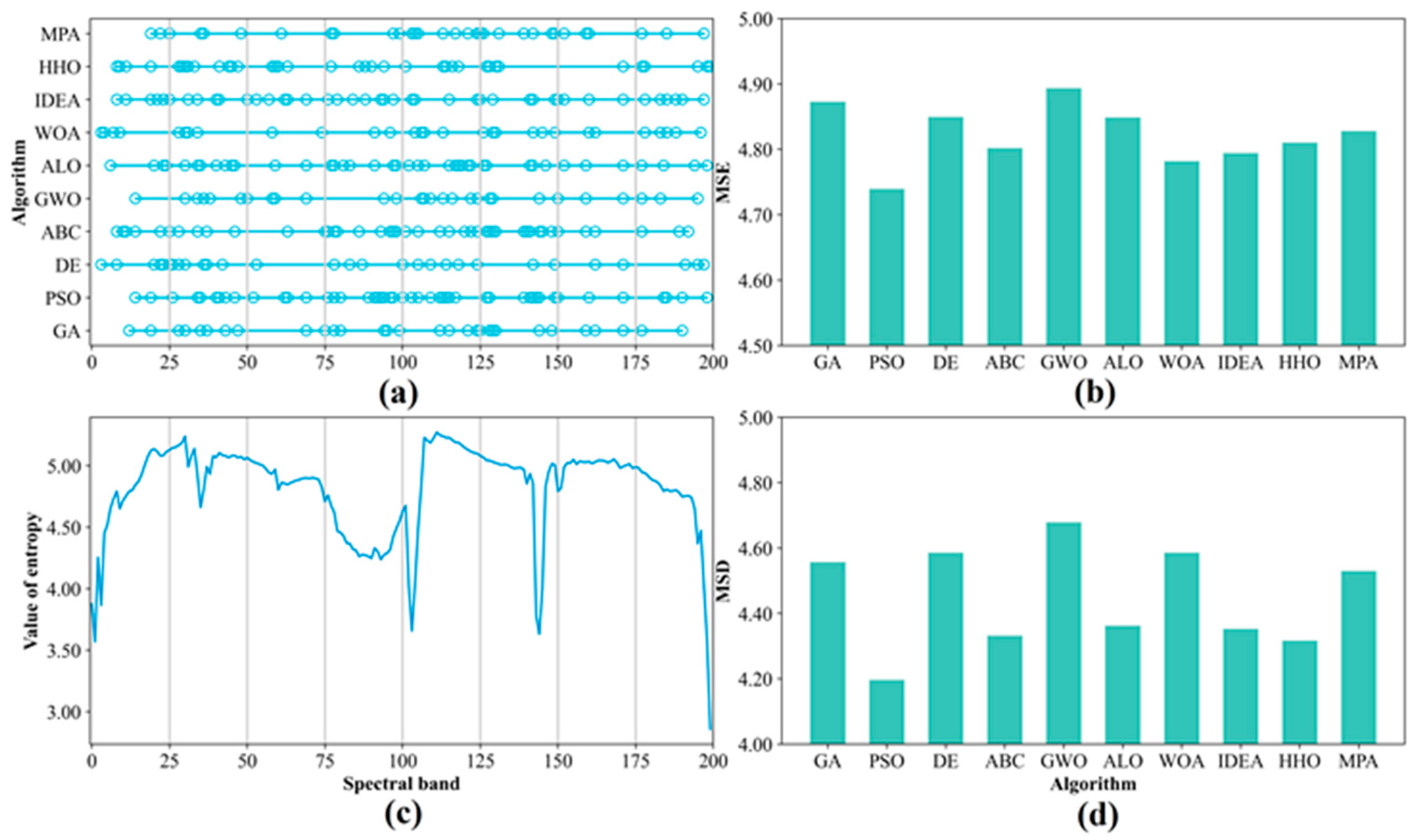
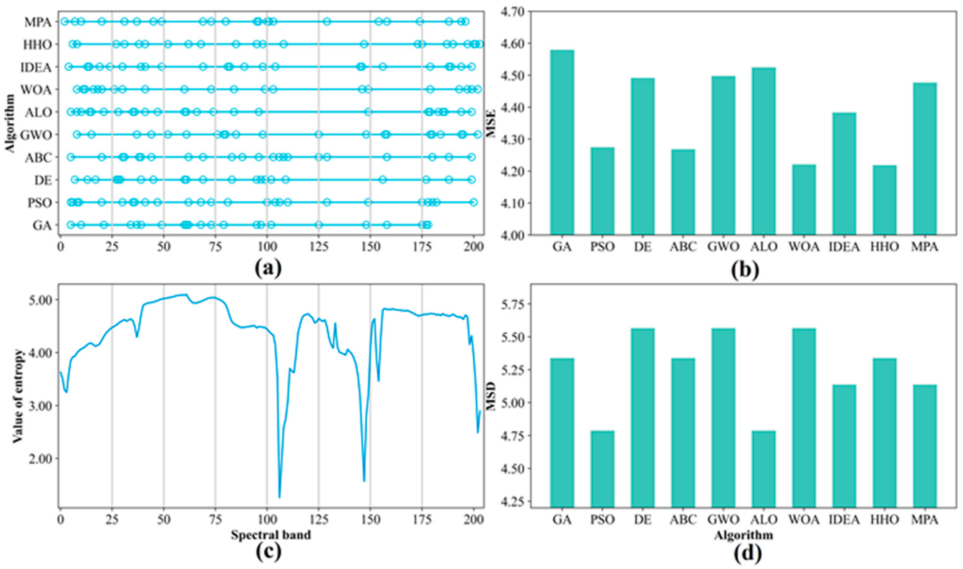
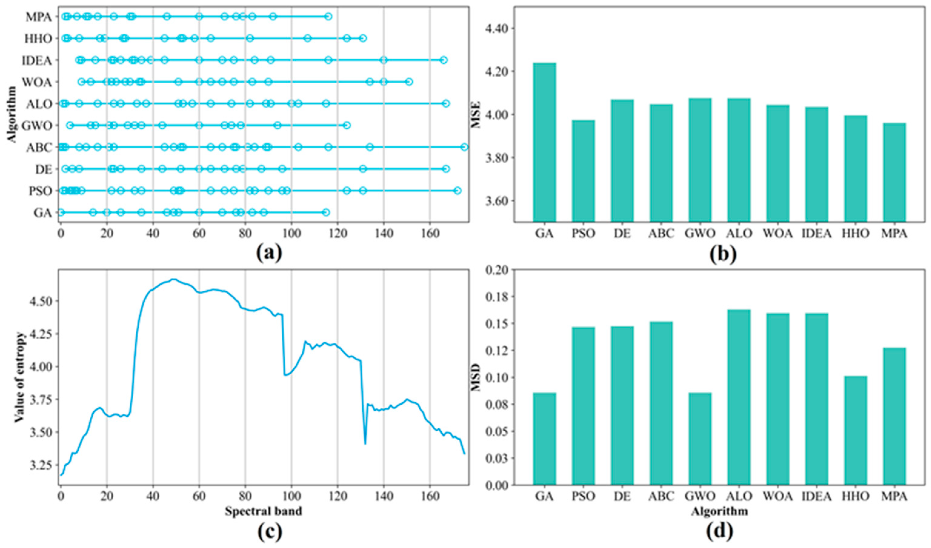
The performances of the F–W–SIEAs on the different datasets are different. For instance, the fitness of F–W–PSO is lower than F–W–ABC on the Indian Pines data but higher than F–W–ABC on the Salinas and KSC datasets. Moreover, the fitness value of F–W–ALO is higher than F–W–IDEA on the Indian Pines data, but the other two datasets have similar fitness values. F–W–ALO has higher fitness values than F–W–IDEA on the Indian Pines data, but the two algorithms have similar fitness values on the other datasets. This result may be explained by the different spectral complexity of the different datasets [45]. As shown in Figure 4, the Indian Pines dataset has a more complex scene than the other datasets. Moreover, several classes have similar spectral characteristics; in other words, the classification difficulty of the datasets is different, which may be the direct cause of the various performances of F–W–SIEAs on different datasets. In general, the findings indicate that F–W–GA and F–W–GWO have similar optimization abilities and perform the best on all the datasets. They can achieve the highest OAs by compressing above 85% of the bands from the original HSIs, but F–W–GWO requires less runtime than F–W–GA. Therefore, F–W–GA and F–W–GWO are preferred for HSI FS, especially in complex scenes. If considering the runtime, F–W–GWO should be the best choice.
Many SIEAs are proposed yearly, and these algorithms are often generated by simulating natural or manmade processes. Invariably, the authors of such papers promise that their new SIEA is superior to algorithms previously published in the literature. However, contrary to expectations, we do not find evidence that the newer the SIEA, the better the optimization results (i.e., OA and NB). For instance, the just emerging SIEAs (e.g., HHO) do not perform better than SIEAs (e.g., GA and GWO) proposed earlier on HSI classification. A possible explanation for the results is the new SIEAs can solve many numerical optimization problems. Still, there are a few exceptions; for instance, they may not be reliable for some specific real-world problems [27]. Choosing the appropriate approach is crucially important rather than directly applying the latest algorithm. Therefore, when using SIEAs for specific issues, it is necessary to conduct the pre-experiments to determine how well they work, and wrong choices of optimization methods may lead to unsatisfactory results. This pre-experiment practice has also been suggested in selecting suitable filter-based methods [12]. In addition, the academic community has proposed considerable SIEAs, where many algorithms may only be proposed but are not widely used in various real-world problems. Hence, the future of the metaheuristic field should perhaps not be to keep creating new SIEAs, but to apply and improve existing ones. Future studies may focus on the different algorithms’ operational mechanisms [58]. Brezocnik et al. [30] also suggest that combining the strengths of different SIEAs to improve existing ones is significant for the metaheuristic field.
Another interesting aspect of this study would be finding that the performance of the commonly used FS techniques is also related to the HSI scene. For instance, for the Indian Pines dataset, the representative F–W–SIEAs obtain much higher OAs than the commonly used filter algorithms; meanwhile, for the KSC dataset with simple scenes, several F–W–SIEAs do not achieve higher OAs than the filter algorithms. Furthermore, it is well-known that the wrapper methods are much more time-consuming than the filter methods. Therefore, we can first choose whether to use filter or wrapper methods depending on the complexity of the HSI. If the image is a somewhat “easy” dataset and the task is urgent, we should try the filter methods rather than wrapper methods, as these methods can basically obtain the desired results and save much runtime.
This study also has some limitations. To make a fair comparison of these ten algorithms, we used MATLAB to build an experimental environment based on the same computer platform. We reproduced the algorithms according to the corresponding papers. However, the performance of one SIEA depends not only on factors related to those mentioned above (i.e., the specific code, the programming language, and the software or hardware used) but also on other factors beyond the control of the algorithm (e.g., individual coding skills). In addition, we compared the performances of a total of ten SIEAs for HSI FS. In fact, there are still many other excellent SIEAs in existence, but a discussion of all SIEAs lies beyond our ability.

6. Conclusions

To compensate for the drawbacks of existing filter–wrapper models and compare the performances of various SIEAs for HSI FS, we proposed a novel filter–wrapper framework to optimize the SVM and classify HSIs. The framework integrates several commonly used filter methods in the filter component and applies each of the ten SIEAs for comparison in the wrapper component. Based on the classification results of these F–W–SIEAs, we compared different methods’ performances in regard to the accuracy, number of selected bands, convergence rate, and relative runtime. Our results show the following:
For the three HSI datasets, most F–W–SIEAs can obtain better results than the corresponding pure SIEA wrappers. Specifically, each F–W–SIEA can obtain higher classification accuracy with a smaller feature subset size in a shorter time than the pure SIEA wrapper. In other words, the framework can combine with different SIEAs to reduce their computational complexity and enhance their classification performances on HSI classification. This framework also provides a new hybrid idea for other FS problems.
The performance of different F–W–SIEAs on different datasets varies slightly, as influenced by the algorithms’ optimization abilities, the complexity of the study area, etc. Specifically, the accuracy, the number of selected bands, the convergence rate, and the relative runtime of the ten F–W–SIEAs are different, but some have similar optimization abilities. On average, among the ten F–W–SIEAs, F–W–GA and F–W–GWO have similar optimization abilities and perform the best on the datasets. They achieve the highest OAs by reducing above 85% of the bands from original HSIs, but F–W–GWO requires the least runtime among the ten. F–W–MPA is also excellent, second only to the above two algorithms and slightly better than the F–W–DE. While F–W–ALO, F–W–IDEA, and F–W–WOA have moderate optimization capabilities, the F–W–IDEA takes the most runtime of all methods. The algorithms that perform poorly overall are F–W–PSO, F–W–ABC, and F–W–HHO. The difference in the optimization results between the ten methods becomes even more significant in more complex scenes (e.g., Indian Pines). We also find that the number of iterations to reach convergence differs between algorithms. In general, the better the algorithm’s optimization ability, the more uniform the band distribution and the higher the MSE and MSD of the selected bands. Despite the differences in optimization ability between the ten F–W–SIEAs, four representative algorithms at different levels still perform better than commonly used FS methods (e.g., CMIM, mRMR, and ReliefF) overall, especially in complex scenes.
This paper is a reference for people who would like to conduct FS on HSIs by applying SIEAs under the proposed framework. It can help them choose appropriate algorithms according to their computational resources, image scenes, etc. Future studies will use our analyses to combine different models to enhance their classification performance. Our analyses could also be extended by considering other FS methods apart from the ten SIEAs, which were out of scope for this analysis. In addition, we used various SIEAs to optimize the SVM classifier for comparison. We will also consider the effect of SIEAs on optimizing other advanced classifiers (e.g., K-Nearest Neighbor and Artificial Neural Networks).

Author Contributions

Conceptualization, X.Z. and Y.S.; methodology, Y.S.; software, Y.S.; validation, Y.S. and J.L.; formal analysis, X.Z., J.L., D.L. and P.W.; writing—original draft preparation, Y.S.; writing—review and editing, X.Z., J.L., D.L. and P.W. All authors have read and agreed to the published version of the manuscript.

Funding

This research was funded by the National Natural Science Foundation of China (Grant No. 72033005); the Open Fund of Key Laboratory of Urban Land Resources Monitoring and Simulation; the Ministry of Natural Resources (Grant No. KF-2020-05-063); the 2021 Graduate Innovation Fund Project of China University of Geosciences, Beijing (Grant No. YB2021YC017); and 2021 Graduate Innovation Fund Project of China University of Geosciences, Beijing (Grant No. ZY2021YC010).

Conflicts of Interest

The authors declare no conflict of interest.

References

  1. Khan, M.J.; Khan, H.S.; Yousaf, A.; Khurshid, K.; Abbas, A. Modern Trends in Hyperspectral Image Analysis: A Review. IEEE Access 2018, 6, 14118–14129. [Google Scholar] [CrossRef]
  2. Medus, L.D.; Saban, M.; Frances-Villora, J.V.; Bataller-Mompean, M.; Rosado-Munoz, A. Hyperspectral image classification using CNN: Application to industrial food packaging. Food Control 2021, 125, 107962. [Google Scholar] [CrossRef]
  3. Ghamisi, P.; Yokoya, N.; Li, J.; Liao, W.; Liu, S.; Plaza, J.; Rasti, B.; Plaza, A. Advances in Hyperspectral Image and Signal Processing: A Comprehensive Overview of the State of the Art. IEEE Geosci. Remote Sens. Mag. 2017, 5, 37–78. [Google Scholar] [CrossRef] [Green Version]
  4. Wang, L.; Zhao, C. Hyperspectral Image Processing; Springer: Berlin/Heidelberg, Germany, 2016. [Google Scholar]
  5. Taskin, G.; Kaya, H.; Bruzzone, L. Feature Selection Based on High Dimensional Model Representation for Hyperspectral Images. IEEE Trans. Image Process. 2017, 26, 2918–2928. [Google Scholar] [CrossRef]
  6. Kalidindi, K.R.; Gottumukkala, P.S.V.; Davuluri, R. Derivative-based band clustering and multi-agent PSO optimization for optimal band selection of hyper-spectral images. J. Supercomput. 2020, 76, 5873–5898. [Google Scholar] [CrossRef]
  7. Wang, J.; Zhou, J.; Huang, W. Attend in Bands: Hyperspectral Band Weighting and Selection for Image Classification. IEEE J. Sel. Top. Appl. Earth Obs. Remote Sens. 2019, 12, 4712–4727. [Google Scholar] [CrossRef]
  8. Li, S.; Wu, H.; Wan, D.; Zhu, J. An effective feature selection method for hyperspectral image classification based on genetic algorithm and support vector machine. Knowl. Based Syst. 2011, 24, 40–48. [Google Scholar] [CrossRef]
  9. Ding, X.; Li, H.; Yang, J.; Dale, P.; Chen, X.; Jiang, C.; Zhang, S. An Improved Ant Colony Algorithm for Optimized Band Selection of Hyperspectral Remotely Sensed Imagery. IEEE Access 2020, 8, 25789–25799. [Google Scholar] [CrossRef]
  10. Wang, M.; Wu, C.; Wang, L.; Xiang, D.; Huang, X. A feature selection approach for hyperspectral image based on modified ant lion optimizer. Knowl. Based Syst. 2019, 168, 39–48. [Google Scholar] [CrossRef]
  11. Unler, A.; Murat, A.; Murat, A. mr(2)PSO: A maximum relevance minimum redundancy feature selection method based on swarm intelligence for support vector machine classification. Inf. Sci. 2011, 181, 4625–4641. [Google Scholar] [CrossRef]
  12. Bommert, A.; Sun, X.; Bischl, B.; Rahnenfuehrer, J.; Lang, M. Benchmark for filter methods for feature selection in high-dimensional classification data. Comput. Stat. Data Anal. 2019, 143, 106839. [Google Scholar] [CrossRef]
  13. Xue, X.; Wu, Z. A novel ensemble-based wrapper method for feature selection using extreme learning machine and genetic algorithm. Knowl. Inf. Syst. 2018, 57, 389–412. [Google Scholar] [CrossRef]
  14. Hancer, E. Differential evolution for feature selection: A fuzzy wrapper–filter approach. Soft Comput. 2019, 23, 5233–5248. [Google Scholar] [CrossRef]
  15. Xie, F.; Li, F.; Lei, C.; Ke, L. Representative Band Selection for Hyperspectral Image Classification. ISPRS Int. J. Geo-Inf. 2018, 7, 338. [Google Scholar] [CrossRef] [Green Version]
  16. Zhang, W.; Li, X.; Zhao, L. Discovering the Representative Subset with Low Redundancy for Hyperspectral Feature Selection. Remote Sens. 2019, 11, 1341. [Google Scholar] [CrossRef] [Green Version]
  17. Ghosh, A.; Datta, A.; Ghosh, S. Self-adaptive differential evolution for feature selection in hyperspectral image data. Appl. Soft Comput. 2013, 13, 1969–1977. [Google Scholar] [CrossRef]
  18. Wang, M.; Wu, C.; Chen, M.; Chen, B.; Jiang, Y. A band selection approach based on Levy sine cosine algorithm and alternative distribution for hyperspectral image. Int. J. Remote Sens. 2019, 41, 3429–3445. [Google Scholar] [CrossRef]
  19. Alomari, O.A.; Khader, A.T.; Al-Betar, M.A.; Awadallah, M.A. A novel gene selection method using modified MRMR and hybrid bat-inspired algorithm with beta-hill climbing. Appl. Intell. 2018, 48, 4429–4447. [Google Scholar] [CrossRef]
  20. El Akadi, A.; Amine, A.; El Ouardighi, A.; Aboutajdine, D. A two-stage gene selection scheme utilizing MRMR filter and GA wrapper. Knowl. Inf. Syst. 2011, 26, 487–500. [Google Scholar] [CrossRef]
  21. Pirgazi, J.; Alimoradi, M.; Abharian, T.E.; Olyaee, M.H. An Efficient hybrid filter-wrapper metaheuristic-based gene selection method for high dimensional datasets. Sci. Rep. 2019, 9, 18580. [Google Scholar] [CrossRef]
  22. Singh, P.S.; Karthikeyan, S. Enhanced classification of remotely sensed hyperspectral images through efficient band selection using autoencoders and genetic algorithm. Neural Comput. Appl. 2021, 1–12. [Google Scholar] [CrossRef]
  23. Chiang, H.-S.; Sangaiah, A.K.; Chen, M.-Y.; Liu, J.-Y. A Novel Artificial Bee Colony Optimization Algorithm with SVM for Bio-inspired Software-Defined Networking. Int. J. Parallel Program. 2020, 48, 310–328. [Google Scholar] [CrossRef]
  24. Deng, W.; Yao, R.; Zhao, H.; Yang, X.; Li, G. A novel intelligent diagnosis method using optimal LS-SVM with improved PSO algorithm. Soft Comput. 2019, 23, 2445–2462. [Google Scholar] [CrossRef]
  25. Santos, C.E.; Sampaio, R.C.; Coelho, L.d.S.; Bestard, G.A.; Llanos, C.H. Multi-objective adaptive differential evolution for SVM/SVR hyperparameters selection. Pattern Recognit. 2021, 110, 107649. [Google Scholar] [CrossRef]
  26. Zhou, T.; Lu, H.; Wang, W.; Yong, X. GA-SVM based feature selection and parameter optimization in hospitalization expense modeling. Appl. Soft Comput. 2019, 75, 323–331. [Google Scholar] [CrossRef]
  27. Piotrowski, A.P.; Napiorkowski, M.J.; Napiorkowski, J.J.; Rowinski, P.M. Swarm Intelligence and Evolutionary Algorithms: Performance versus speed. Inf. Sci. 2016, 384, 34–85. [Google Scholar] [CrossRef]
  28. Xie, F.; Li, F.; Lei, C.; Yang, J.; Zhang, Y. Unsupervised band selection based on artificial bee colony algorithm for hyperspectral image classification. Appl. Soft Comput. 2018, 75, 428–440. [Google Scholar] [CrossRef]
  29. Wang, M.; Liu, W.; Chen, M.; Huang, X.; Han, W. A band selection approach based on a modified gray wolf optimizer and weight updating of bands for hyperspectral image. Appl. Soft Comput. 2021, 112, 107805. [Google Scholar] [CrossRef]
  30. Brezocnik, L.; Fister, I., Jr.; Podgorelec, V. Swarm Intelligence Algorithms for Feature Selection: A Review. Appl. Sci. 2018, 8, 1521. [Google Scholar] [CrossRef] [Green Version]
  31. Qi, C.; Zhou, Z.; Sun, Y.; Song, H.; Hu, L.; Wang, Q. Feature selection and multiple kernel boosting framework based on PSO with mutation mechanism for hyperspectral classification. Neurocomputing 2016, 220, 181–190. [Google Scholar] [CrossRef]
  32. Chen, C.L.P.; Zhang, T.; Chen, L.; Tam, S.C. I-Ching Divination Evolutionary Algorithm and its Convergence Analysis. IEEE Trans. Cybern. 2016, 47, 2–13. [Google Scholar] [CrossRef]
  33. Heidari, A.A.; Mirjalili, S.; Faris, H.; Aljarah, I.; Mafarja, M.; Chen, H. Harris hawks optimization: Algorithm and applications. Future Gener. Comput. Syst. 2019, 97, 849–872. [Google Scholar] [CrossRef]
  34. Faramarzi, A.; Heidarinejad, M.; Mirjalili, S.; Gandomi, A.H. Marine Predators Algorithm: A nature-inspired metaheuristic. Expert Syst. Appl. 2020, 152, 113377. [Google Scholar] [CrossRef]
  35. Battitti, R. Using mutual information for selecting features in supervised neural net learning. IEEE Trans. Neural Netw. 1994, 5, 537–550. [Google Scholar] [CrossRef] [Green Version]
  36. Kiktova-Vozarikova, E.; Juhar, J.; Cizmar, A. Feature selection for acoustic events detection. Multimed. Tools Appl. 2015, 74, 4213–4233. [Google Scholar] [CrossRef]
  37. Zhang, Y.; Zhang, Z. Feature subset selection with cumulate conditional mutual information minimization. Expert Syst. Appl. 2012, 39, 6078–6088. [Google Scholar] [CrossRef]
  38. Radovic, M.; Ghalwash, M.; Filipovic, N.; Obradovic, Z. Minimum redundancy maximum relevance feature selection approach for temporal gene expression data. BMC Bioinform. 2017, 18, 9. [Google Scholar] [CrossRef] [Green Version]
  39. Sarkar, J.P.; Saha, I.; Sarkar, A.; Maulik, U. Machine learning integrated ensemble of feature selection methods followed by survival analysis for predicting breast cancer subtype specific miRNA biomarkers. Comput. Biol. Med. 2021, 131, 104244. [Google Scholar] [CrossRef]
  40. Brown, G.; Pocock, A.; Zhao, M.-J.; Lujan, M. Conditional Likelihood Maximisation: A Unifying Framework for Information Theoretic Feature Selection. J. Mach. Learn. Res. 2012, 13, 27–66. [Google Scholar]
  41. Robnik-Sikonja, M.; Kononenko, I. Theoretical and empirical analysis of ReliefF and RReliefF. Mach. Learn. 2003, 53, 23–69. [Google Scholar] [CrossRef] [Green Version]
  42. Lin, Z.; Zhang, G. Genetic algorithm-based parameter optimization for EO-1 Hyperion remote sensing image classification. Eur. J. Remote Sens. 2020, 53, 124–131. [Google Scholar] [CrossRef]
  43. Hsu, C.; Lin, C. A comparison of methods for multiclass support vector machines. IEEE Trans. Neural Netw. 2002, 13, 415–425. [Google Scholar] [CrossRef] [Green Version]
  44. Wainer, J.; Fonseca, P. How to tune the RBF SVM hyperparameters? An empirical evaluation of 18 search algorithms. Artif. Intell. Rev. 2021, 54, 4771–4797. [Google Scholar] [CrossRef]
  45. Zhu, X.; Li, N.; Pan, Y. Optimization performance comparison of three different group intelligence algorithms on a SVM for hyperspectral imagery classification. Remote Sens. 2019, 11, 734. [Google Scholar] [CrossRef] [Green Version]
  46. Cai, Y.; Liu, X.; Cai, Z. BS-Nets: An End-to-End Framework for Band Selection of Hyperspectral Image. IEEE Trans. Geosci. Remote Sens. 2019, 58, 1969–1984. [Google Scholar] [CrossRef] [Green Version]
  47. Landgrebe, D.A.; Biehl, L.L. MultiSpec—A Tool for Multispectral-Hyperspectral Image Data Analysis. Comput. Geosci. 2002, 28, 1153–1159. [Google Scholar] [CrossRef]
  48. Plaza, A.; Martinez, P.; Plaza, J.; Perez, R. Dimensionality reduction and classification of hyperspectral image data using sequences of extended morphological transformations. IEEE Trans. Geosci. Remote Sens. 2005, 43, 466–479. [Google Scholar] [CrossRef] [Green Version]
  49. Rajan, S.; Ghosh, J.; Crawford, M.M. An active learning approach to hyperspectral data classification. IEEE Trans. Geosci. Remote Sens. 2007, 46, 1231–1242. [Google Scholar] [CrossRef]
  50. Mountrakis, G.; Im, J.; Ogole, C. Support vector machines in remote sensing: A review. ISPRS J. Photogramm. Remote Sens. 2011, 66, 247–259. [Google Scholar] [CrossRef]
  51. Velasco-Forero, S.; Manian, V. Improving Hyperspectral Image Classification Using Spatial Preprocessing. IEEE Geosci. Remote Sens. Lett. 2009, 6, 297–301. [Google Scholar] [CrossRef]
  52. AhmedMedjahed, S.; Ouali, M. Band selection based on optimization approach for hyperspectral image classification. Egypt. J. Remote Sens. Space Sci. 2018, 21, 413–418. [Google Scholar] [CrossRef]
  53. Zhang, X.; Lin, Q.; Mao, W.; Liu, S.; Dou, Z.; Liu, G. Hybrid Particle Swarm and Grey Wolf Optimizer and its application to clustering optimization. Appl. Soft Comput. 2021, 101, 107061. [Google Scholar] [CrossRef]
  54. Georganos, S.; Grippa, T.; Vanhuysse, S.; Lennert, M.; Shimoni, M.; Kalogirou, S.; Wolff, E. Less is more: Optimizing classification performance through feature selection in a very-high-resolution remote sensing object-based urban application. GISci. Remote Sens. 2018, 35, 221–242. [Google Scholar] [CrossRef]
  55. Loew, F.; Michel, U.; Dech, S.; Conrad, C. Impact of feature selection on the accuracy and spatial uncertainty of per-field crop classification using Support Vector Machines. ISPRS J. Photogramm. Remote Sens. 2013, 85, 102–119. [Google Scholar] [CrossRef]
  56. Plaza, A.; Benediktsson, J.A.; Boardman, J.W.; Brazile, J.; Bruzzone, L.; Camps-Valls, G.; Chanussot, J.; Fauvel, M.; Gamba, P.; Gualtieri, A.; et al. Recent advances in techniques for hyperspectral image processing. Remote Sens. Environ. 2007, 113, S110–S122. [Google Scholar] [CrossRef]
  57. Harwat, A.; Hassanien, A.E. Chaotic antlion algorithm for parameter optimization of support vector machine. Appl. Intell. 2018, 38, 670–686. [Google Scholar] [CrossRef]
  58. Soerensen, K. Metaheuristics-the metaphor exposed. Int. Trans. Oper. Res. 2015, 22, 3–18. [Google Scholar] [CrossRef]
Figure 1. Flowchart of the filter–wrapper framework. The framework includes the filter and the wrapper components.
Remotesensing 14 03019 g001
Figure 2. Standard process for optimizing SVM classification based on each SIEA.
Remotesensing 14 03019 g002
Figure 3. The SIEA’s individual structure and its change process example.
Remotesensing 14 03019 g003
Figure 4. Images of the three HSIs. (ac) are the the ground truth of Indian Pines, Salinas, and KSC. (df) are the spectral reflectance curves of Indian Pines, Salinas, and KSC.
Remotesensing 14 03019 g004
Figure 5. The fitness values of the F–W–SIEAs on the different datasets. The bar chart shows the fitness of each on the different datasets, and the line chart shows the mean fitness value.
Remotesensing 14 03019 g005
Figure 6. The relative runtime and number of iterations of different algorithms on (a) the Indian Pines dataset, (b) the Salinas dataset, and (c) the KSC dataset.
Remotesensing 14 03019 g006
Figure 7. Analysis of the selected bands on the Indian Pines: (a) selected bands from the methods, (b) MSE value, (c) entropy value of each band of the dataset, and (d) MSD value.
Remotesensing 14 03019 g007
Figure 8. Analysis of the selected bands on the Salinas: (a) selected bands from the methods, (b) MSE value, (c) entropy value of each band of the dataset, and (d) MSD value.
Remotesensing 14 03019 g008
Figure 9. Analysis of the selected bands on the KSC: (a) selected bands from the methods, (b) MSE value, (c) entropy value of each band of the dataset, and (d) MSD value.
Remotesensing 14 03019 g009
Figure 10. The average OA (%) and Kappa of these algorithms on the three HSIs.
Remotesensing 14 03019 g010
Table 1. Specific information of the ten SIEAs.
NameYearComments
GABefore 2000GA is one of the first population-based stochastic algorithm proposed in the history. The main operators of GA are selection, crossover, and mutation.
PSOBefore 2000PSO is a population-based search algorithm and is initialized with random particles. Each particle has its velocity, and particles with velocities dynamically adjust based on historical behaviors. The particles tend to better search areas in this process.
DEBefore 2000DE operates through similar computational steps, as employed by the standard GA. However, DE upgrades the population members with the scaled differences of randomly selected and distinct population members.
ABC2005In ABC, the artificial bees contain three groups: employed bees, onlookers, and scouts. The number of employed bees is equal to the number of food sources, and the employed bee of an abandoned food source becomes a scout.
GWO2014GWO simulates the leadership hierarchy and hunting mechanism of grey wolves in nature. Four types of grey wolves, namely alpha, beta, delta, and omega, are employed for simulating the leadership hierarchy. The three main steps include hunting, searching for prey, encircling prey, and attacking prey.
ALO2015ALO mimics the hunting mechanism of antlions in nature. It involves five main steps: the random walk of ants, building traps, entrapment of ants in traps, catching preys, and re-building traps.
WOA2016WOA is a nature-inspired algorithm that mimics humpback whales’ social behavior, first by chasing the prey with random or the best search agent and second by simulating the bubble-net hunting strategy.
IDEA2017IDEA has three operators evolved from I-Ching transformations, namely the intrication operator, turnover operator, and mutual operator. These operators are flexible in the evolution procedure.
HHO2019HHO is inspired by the cooperative behavior and chasing style of Harris’ hawks in nature. Several hawks cooperatively pounce a prey from different directions in an attempt to surprise it. They can reveal many chasing patterns based on the dynamic nature of scenarios and escaping patterns of the prey.
MPA2020MPA is inspired by the foraging strategy, namely Lévy and Brownian movements in ocean predators, along with optimal encounter rate policy in biological interaction between predator and prey. MPA follows the rules that naturally govern optimal foraging strategy and encounters rate policy between predator and prey.
Table 2. The OA and NB of different algorithms on the Indian Pines dataset.
FrameworkF–WPure
MeasurementOA (%)NBOA (%)NB
GA85.99 ± 0.4331.45 ± 2.9283.81 ± 1.6851.95 ± 4.79
PSO85.64 ± 0.5148.40 ± 6.8784.44 ± 1.0273.60 ± 5.24
DE85.76 ± 0.6137.35 ± 4.0683.95 ± 0.9262.50 ± 6.46
ABC85.87 ± 0.6447.15 ± 3.8984.47 ± 0.6774.70 ± 6.85
GWO86.00 ± 0.4129.00 ± 1.8383.79 ± 0.5044.25 ± 1.33
ALO84.79 ± 0.9437.65 ± 7.3583.49 ± 0.9447.00 ± 9.98
WOA83.51 ± 0.9530.05 ± 6.0583.47 ± 1.2150.25 ± 3.93
IDEA85.06 ± 0.7943.55 ± 7.5983.73 ± 1.0860.65 ± 5.36
HHO83.35 ± 1.2432.25 ± 8.2283.00 ± 0.8952.60 ± 7.50
MPA85.18 ± 0.9831.15 ± 7.0083.67 ± 0.8445.25 ± 8.22
Table 3. The OA and NB of different algorithms on the Salinas dataset.
FrameworkF–WPure
MeasurementOA (%)NBOA (%)NB
GA93.34 ± 0.2820.80 ± 0.9793.30 ± 0.2527.35 ± 3.85
PSO93.07 ± 0.2725.15 ± 3.9692.91 ± 0.2049.50 ± 6.55
DE93.16 ± 0.1821.70 ± 1.1493.20 ± 0.1635.75 ± 1.56
ABC93.05 ± 0.2125.55 ± 2.8293.23 ± 0.1850.50 ± 6.35
GWO93.28 ± 0.1920.25 ± 0.7693.25 ± 0.2133.15 ± 2.56
ALO92.87 ± 0.2524.10 ± 1.3392.85 ± 0.3345.55 ± 2.75
WOA92.53 ± 0.2921.05 ± 3.6192.33 ± 0.3939.35 ± 5.86
IDEA93.14 ± 0.1624.45 ± 2.8092.33 ± 0.7255.30 ± 3.53
HHO92.65 ± 0.3124.05 ± 1.8392.35 ± 0.6952.00 ± 3.93
MPA93.10 ± 0.5724.10 ± 1.3493.15 ± 0.5238.25 ± 5.31
Table 4. The OA and NB of different algorithms on the KSC dataset.
FrameworkF–WPure
MeasurementOA (%)NBOA (%)NB
GA93.33 ± 0.2614.70 ± 0.6592.74 ± 0.5532.05 ± 3.96
PSO93.10 ± 0.6524.20 ± 4.7192.89 ± 0.5658.75 ± 8.51
DE93.11 ± 0.3617.70 ± 0.9092.81 ± 0.2240.90 ± 5.75
ABC92.95 ± 0.2424.05 ± 3.2892.46 ± 0.8758.30 ± 5.68
GWO93.24 ± 0.2115.05 ± 1.2092.55 ± 0.6128.15 ± 1.42
ALO92.52 ± 0.6020.35 ± 1.6892.91 ± 0.1845.10 ± 7.62
WOA91.83 ± 0.6018.45 ± 1.9391.81 ± 0.3736.25 ± 3.46
IDEA92.81 ± 0.7820.05 ± 2.9692.45 ± 2.0250.10 ± 10.62
HHO91.36 ± 1.2016.20 ± 1.6691.33 ± 5.4640.15 ± 1.98
MPA92.78 ± 0.7816.60 ± 1.1192.29 ± 1.3740.65 ± 1.71
Table 5. The mean value of different algorithms on the three datasets.
FrameworkF–WPure
MeasurementOA (%)NBOA (%)NB
GA90.8922.3289.9537.12
PSO90.6032.5890.0860.62
DE90.6825.5889.9946.38
ABC90.6232.2590.3261.17
GWO90.8421.4389.8635.18
ALO90.0627.3789.7545.88
WOA89.2923.1889.2041.95
IDEA90.3429.3589.5055.35
HHO89.1224.1788.8948.25
MPA90.3523.9589.7041.38
Mean value90.2826.2289.7347.33
Table 6. The OA, Kappa coefficient, and accuracy of each class for Indian Pines dataset.
No.FBMIFSJMICMIMmRMRReliefFF–W–GAF–W–MPAF–W–IDEAF–W–PSO
154.0540.5467.5762.1654.0556.7691.8989.1978.3889.19
280.8264.6267.2560.5174.5270.3283.4582.2279.4279.07
378.9251.8162.6550.6057.5363.2574.4074.1074.4064.61
472.6363.6868.4254.7467.9058.4280.0078.9565.7975.26
594.5692.2388.8688.0892.4989.3895.6094.0496.3790.16
696.2394.0193.6695.2196.5890.5895.2197.0996.2396.92
777.2781.8286.3672.7386.3681.8290.9190.9181.8286.36
898.9595.2997.6496.6096.0792.9397.9197.9196.8697.38
931.2543.7525.0050.0081.2543.7537.5075.0062.5093.75
1079.9564.2772.3761.9570.4475.8479.8282.0178.9273.52
1187.8880.8080.0477.7082.4379.7986.3085.2983.5586.15
1282.0748.1058.0251.0654.4365.1985.8784.3973.0081.01
1397.5696.3496.9598.7899.3991.46100.0099.3998.7897.56
1495.2693.5896.2594.0791.9094.2794.6694.2795.4695.85
1563.7566.0249.1949.1968.9344.0167.3166.6759.2253.72
1683.7887.8486.4985.1490.5483.7889.1987.8489.1985.14
OA (%)86.0275.6477.8773.4679.2977.7986.3386.0183.7483.37
Kappa0.84030.72060.74720.69590.76270.74630.84400.84050.81450.8094
Table 7. The OA, Kappa coefficient, and accuracy of each class for Salinas dataset.
No.FBMIFSJMICMIMmRMRReliefFF–W–GAF–W–MPAF–W–IDEAF–W–PSO
199.6999.0799.5699.2599.3299.3899.9499.8899.7599.69
299.3397.4899.2399.0698.2698.7999.3099.3399.1399.36
399.6292.4795.7696.2194.2490.8997.7998.4299.1899.18
499.1098.5799.1098.8398.6698.8399.0199.2899.1998.66
599.1196.9296.5996.7396.9796.5597.9598.4698.5198.41
699.9799.9799.6599.6299.9799.4399.9799.9199.9799.97
799.7998.1899.6299.5198.3299.4199.5599.5899.5899.65
888.5087.6584.0485.5489.4985.4589.4888.0187.0987.57
999.9299.2198.5599.3699.4497.4099.6699.7699.7499.78
1097.9089.2595.1294.8990.6989.4096.4597.0396.2296.99
1199.0690.9893.6895.2088.8888.0698.0197.6699.1898.36
1299.8196.3099.2299.1696.6999.2999.7499.5599.6899.42
1399.7397.5499.7399.7398.3698.3699.86100.0099.5999.86
1498.6096.3897.7898.4896.8598.4899.1899.1899.1898.83
1568.7555.1361.7767.5857.9151.3877.1275.6173.2572.22
1698.5597.7999.2498.8299.2498.2099.5299.2499.1099.17
OA (%)93.0189.3790.3991.5790.4388.4094.1193.6893.1693.14
Kappa0.92210.88130.89280.90600.89310.87050.93440.92960.92380.9236
Table 8. The OA, Kappa coefficient, and accuracy of each class for the KSC dataset.
No.FBMIFSJMICMIMmRMRReliefFF–W–GAF–W–MPAF–W–IDEAF–W–PSO
195.4095.9095.5797.5496.2297.3797.2196.3996.8896.39
289.6987.1187.6389.1885.5781.9693.3087.6383.5188.14
393.1787.8186.3491.7192.6888.7890.2492.6893.1789.76
479.2158.4281.6882.1876.7361.8877.2371.7880.6985.64
562.7940.3164.3469.7760.4758.9271.3261.2466.6769.77
668.3157.3856.2862.3064.4851.9171.5969.9563.3949.18
788.1091.6795.2495.2494.0586.9190.4894.0592.8688.10
891.5987.2591.5989.8689.8678.2691.3092.4691.0192.46
997.3696.1596.1596.6497.1294.4796.1596.8896.3996.39
1098.7698.7699.6998.7695.9893.5098.7698.7698.4598.45
1198.5194.9396.1297.3197.3188.6698.5198.2196.1297.31
1296.0297.0292.2998.2697.2691.7996.0297.0295.2793.04
13100.00100.00100.00100.00100.00100.00100.00100.00100.00100.00
OA (%)93.1690.0791.9493.5292.4688.1893.6793.0792.7392.32
Kappa0.92380.88930.91090.92780.91600.86810.92940.92280.91890.9144
Publisher’s Note: MDPI stays neutral with regard to jurisdictional claims in published maps and institutional affiliations.

