Article

Fast Approach for SAR Imaging of Ground-Based Moving Targets Based on Range Azimuth Joint Processing

1
The 38th Research Institute of China Electronics Technology Group Corporation, Hefei 230088, China
2
School of Microelectronics and Communication Engineering, Chongqing University, Chongqing 400044, China
3
Chongqing Key Laboratory of Space Information Network and Intelligent Information Fusion, Chongqing University, Chongqing 400044, China
4
Chongqing Key Laboratory of Mobile Communications Technology, Chongqing University of Posts and Telecommunications, Chongqing 400065, China
*
Author to whom correspondence should be addressed.
Remote Sens. 2022, 14(13), 2965; https://doi.org/10.3390/rs14132965
Submission received: 24 May 2022 / Revised: 19 June 2022 / Accepted: 19 June 2022 / Published: 21 June 2022

Abstract

:
The synthetic aperture radar (SAR) images of a moving target may be out of focus, given the motions of a non-cooperative target. Doppler ambiguities, including the Doppler center blur and spectrum ambiguity, will easily appear due to the limitations of pulse repetition frequency, which causes difficulty in moving-target imaging. Therefore, a robust fast Doppler ambiguity approach for SAR imaging of a ground-based moving target using range azimuth joint processing (RAJP) is presented. Firstly, the use of RAJP, based on a two-dimensional cross-correlation function and linear range cell migration (LRCM) compensation function, is proposed to simultaneously obtain the first- and second-order phase parameters in the fast-time and azimuth-frequency domains. Then, a corresponding azimuth reference function is constructed to image the moving target. Additionally, a principal component analysis-based operation is introduced to solve the mismatch with the LRCM compensation function. The couplings between the range and azimuth and between the first- and second-order parameters can be simultaneously decoupled by the proposed RAJP operation, which simplifies the processing steps. The developed approach can simultaneously obtain the first- and second-order parameters in the fast-time and azimuth-frequency domains, which avoids the propagation error of parameter estimation caused by the stepwise processing operation. The proposed method is relatively fast, given the need for fewer processing steps. The presented approach is robust in terms of Doppler ambiguity and handles the blind speed sidelobe well. In this study, simulated and real data are processed to verify the proposed approach.

Graphical Abstract

1. Introduction

Synthetic aperture radar (SAR) is a technique that is receiving more and more attention worldwide nowadays, given that it is capable of imaging the observed scenes of interest, regardless of weather conditions, both day and night [1,2,3,4,5,6]. SAR has been widely employed in different applications, such as environmental observation, traffic monitoring, sea-surface surveillance, and antiterrorism. However, moving targets inevitably emerge into the scene of observation. Therefore, ground moving-target imaging (GMTIm) is a research hotspot that has become important in SAR applications, due to the growing demand for moving-target surveillance [7,8,9,10,11,12,13].
Nevertheless, tracking the unpredictable motions (cross- and along-track velocities) of ground-based moving targets will result in range cell migration (RCM) and Doppler frequency broadening (DFB), leading to the severe defocusing of moving targets [14,15]. RCM makes a moving target’s energy defocus along the range dimensions. RCM includes linear RCM (LRCM) and quadratic RCM (QRCM), which are influenced by the cross- and along-track velocities of a moving target, respectively; the DFB induced by the target’s along-track velocity leads to a defocusing effect on a moving target in the azimuth Doppler dimension. Therefore, for the successful imaging of moving targets, the effects of RCM and DFB should be effectively addressed [12,13,14,15].
Recently, the Hough transform [16], Radon transform [17] and axis rotation transform [18] models have been introduced to address LRCM by utilizing the moving target trajectory in the range and azimuth domains. However, these transforms have a huge computational cost, given that they need to run the searching operation for the target trajectory. The Keystone transform (KT) [19,20,21], second-order KT (SKT) [22,23], and Doppler KT (DKT) [24] have been developed to eliminate the LRCM or QRCM of a moving target without searching for the target trajectory. However, these methods (i.e., KT, SKT, and DKT) find it hard to deal with the effect of DFB and suffer from the problem of Doppler ambiguity.
Generally, because of the limitations of the pulse repetition frequency (PRF) of an SAR system, the moving target signal quickly demonstrates a Doppler ambiguity [13,14,15,25]. If the Doppler center shift (DCS) induced by the cross-track velocity of a moving target is larger than PRF/2, a Doppler center blur will be generated. Notably, the potential Doppler spectrum distributions caused by DCS and DFB include the following cases: (1) the Doppler spectrum is entirely located in one PRF band; (2) the Doppler spectrum spans over two PRF bands; (3) the Doppler spectrum occupies several PRF bands. If the target Doppler spectrum is distributed in two or in several PRF bands (i.e., situations (2) and (3)), the moving target signal will exhibit Doppler spectrum splitting, thereby leading to Doppler spectrum ambiguity. These factors (i.e., Doppler center blur and spectrum ambiguity) make moving target imaging become more difficult.
In order to handle the DFB and Doppler ambiguity, a two-dimensional (2-D) frequency-matched filtering (2-DFMF) algorithm [14] has been proposed by exploiting a feature in the range–azimuth frequency domain for a target signal, based on the stationary phase principle. Although this method can efficiently image ground-based moving targets, it ignores the unpredictable motions of a moving target, leading to a loss in coherent accumulation. However, this stationary phase-based algorithm may only be suitable for the scenario of a moving target signal with a large azimuth time-bandwidth product, given that it should obtain the precise 2-D Doppler spectrum using the stationary phase principle. Therefore, the Deramp–Keystone processing (DKP) method [15] has been applied in this study. However, the DKP approach approximately removes the QRCM and DFB by applying the a priori velocity of the radar platform but still neglects the residual correction errors induced by the target’s unknown motions. In [26], a Keystone-based method without searching the Doppler chirp rate has been introduced for considering the unknown motions of a moving target. However, this method addresses the Doppler center blur by using the Doppler ambiguity number-searching operation but is troubled by the effects of Doppler spectrum ambiguity and the residual correction error of QRCM. In an earlier work [27], a segmented KT–Doppler Lv’s transform algorithm, based on Doppler ambiguity number-searching, has been proposed to address the Doppler spectrum ambiguity. Nevertheless, this algorithm validates the finding that if the bandwidth of the target Doppler spectrum exceeds half of the PRF, the Doppler center shifting operation that is utilized to deal with the problem of Doppler spectrum ambiguity will be invalid. The discrete polynomial-phase transform (DPT)-based method [28] has been presented without the problem of Doppler spectrum ambiguity. However, this approach ignores the QRCM induced by the target’s along-track velocity, resulting in a severe defocusing effect.
Additionally, various multi-dimensional searching approaches have been developed for achieving well-focused results; for example, the radon-fractional Fourier transform [29], extended generalized radon Fourier transform [30], polynomial radon–polynomial Fourier transform [31], and the modified KT-matched filtering method [32]. Nevertheless, the computational costs of these algorithms are huge, given the multi-dimensional brute-force parameter searching step included in the implementation procedure. To reduce the computational cost, several algorithms with a one-dimensional searching operation have been proposed; for example, the modified SOKT (MSOKT) [13], improved time-reversal–modified radon Fourier transform (ITRT–MRFT) [33], improved axis rotation–time-reversal transform (IAR–TRT) [9], and modified axis rotation–Lv’s transform [34]. However, these approaches are still troubled by a high computational burden, due to the one-dimensional searching procedure of a moving target. In addition, the MSOKT and ITRT–MRFT approaches suffer from a serious problem with blind speed sidelobe (BSSL), and the IAR–TRT is affected by scaled frequency spectrum aliasing.
Motivated by the previous study, a quicker approach for achieving SAR imaging of ground-based moving targets, based on range azimuth joint processing (RAJP), is presented in his paper. Firstly, an RAJP, based on the 2D cross-correlation function and the presented LRCM compensation function, is proposed to simultaneously obtain the first- and second-order phase parameters in the fast-time and azimuth-frequency domains. Then, an azimuth reference function corresponding to the obtained phase parameters is constructed, to image the moving target in the range–azimuth time domain. In addition, the mismatch of the LRCM compensation function is analyzed, and a principal component analysis (PCA)-based operation is introduced to address this issue (i.e., mismatch of the LRCM compensation function). Simulated data and real data, including spaceborne and airborne real data, are processed to verify the developed approach.
The main contributions of this study can be summarized as follows: (1) the proposed RAJP operation can simultaneously decouple the couplings between the range and azimuth and between first- and second-order parameters, which can simplify the processing steps; (2) the presented method can simultaneously obtain first- and second-order phase parameters in the fast-time and azimuth-frequency domains, which can counteract the propagation error induced by the operation of the stepwise parameter estimation; (3) the proposed method is computationally efficient due to having fewer processing steps; (4) the developed method is robust when faced with Doppler ambiguity, including a Doppler center blur and spectrum ambiguity, and can deal with the BSSL problem; (5) a PCA-based operation is introduced to deal with the LRCM compensation function mismatch, according to an analysis related to the mismatch of the LRCM compensation function.
The rest of this paper is organized as follows. Section 2 presents the signal model and the characteristics of the moving target. Section 3 introduces the proposed algorithm. Section 4 provides some discussions related to the proposed method. Section 5 gives the experimental results, including the simulated, spaceborne, and airborne real data-processing results. Section 6 concludes the paper.

2. Signal Model and Characteristics

2.1. Signal Model

A SAR that is used when in a side-facing strip-map working mode is chosen; Figure 1 illustrates the motion geometric model between a SAR platform with velocity v and a ground moving target on the slant range plane. During the synthesis time T a , the moving target, with cross-track velocity v c and along-track velocity v a , travels from point A to point B. The nearest and instantaneous slant ranges between the SAR and moving target are indicated by R 0 and R s ( t n ) . t n represents the azimuth time.
On the basis of the motion geometry geometric model depicted in Figure 1, R s ( t n ) is written as follows:
R s ( t n ) = ( v t n v a t n ) 2 + ( R 0 v c t n ) 2 .
Then, R s ( t n ) can be expanded according to the Taylor series expansion, and a quadratic term model is utilized, as follows [8,9,13,14,15,22,23,24,25,26,27]:
R s ( t n ) R 0 v c t n + ( v v a ) 2 2 R 0 t n 2 .
It is assumed that the SAR employed the widely used linear frequency modulation signal as the transmitted signal, with the following form:
s t ( t ) = rect ( t T p ) exp ( j 2 π f c t + j 2 π γ t 2 )
where t , T p , f c and γ indicate the fast time, pulse length, carrier frequency and chirp rate of the transmitted signal, respectively, rect ( t T p ) = { 1 ,   | t | T p / 2 0 , | t | > T p / 2   . Then, the received baseband signal of the moving target is expressed as follows [26,27,35]:
s b a s e ( t , t n ) = rect [ t 2 R s ( t n ) c T p ] w ( t n ) exp ( j 2 π γ [ t 2 R s ( t n ) c ] 2 ) × exp [ j 4 π λ R s ( t n ) ]
where c , w ( · ) and λ denote the speed of the electromagnetic wave, azimuth window function, and the wavelength of the transmitted signal, respectively.
After range compression [26,27] and substituting Equation (2) into Equation (4), the received baseband signal, omitting the amplitude in the range- and azimuth-time domain, is written as follows:
s 1 ( t , t n ) = sin c { B [ t 2 ( R 0 v c t n + ( v v a ) 2 2 R 0 t n 2 ) / c ] } w ( t n ) × exp [ j 4 π λ ( R 0 v c t n + ( v v a ) 2 2 R 0 t n 2 ) ]
where B = γ T p is the bandwidth of the transmitted signal. Here, sin c ( x ) = sin ( π x ) / ( π x ) represents the sinc function.

2.2. Signal Characteristics

(1) Range Migration and Doppler Broadening Analysis: as described in the sinc function term of Equation (5), the range time t is coupled with the azimuth time, and the pulse envelope position changes with the azimuth time. Therefore, the target position, offset in the range dimension, is written as follows:
{ Δ R 1 = | v c t n | t n [ T a / 2 , T a / 2 ] = | 2 v c ( T a 2 ) | Δ R 2 = | ( v v a ) 2 2 R 0 t n 2 | t n [ T a / 2 , T a / 2 ] = | ( v v a ) 2 2 R 0 ( T a 2 ) 2 |
where Δ R 1 and Δ R 2 denote the range position offsets induced by t n - and t n 2 -terms, respectively. If Δ R 1 < c / ( 2 B ) , the LRCM will appear. The LRCM is the linear trajectory in the range and azimuth plane. In the meantime, the QRCM will emerge, when Δ R 2 < c / ( 2 B ) . The QRCM is the parabolic trajectory in the range and azimuth plane, which is symmetric with respect to the center point of azimuth time. The total RCM includes LRCM and QRCM. The RCM will ensure that the moving target energy defocuses along the range dimension.
As described in the exponential term of Equation (5), the Doppler frequency offsets (DFO) in the Doppler frequency dimension are expressed as follows:
{ Δ f 1 = | 2 v c / λ | t n [ T a 2 , T a 2 ] = | 2 v c / λ | Δ f 2 = | 2 ( v v a ) 2 R 0 λ t n | t n [ T a 2 , T a 2 ] = | 4 ( v v a ) 2 R 0 λ ( T a 2 ) |
where Δ f 1 and Δ f 2 represent the DFOs caused by t n - and t n 2 -terms, respectively. The target signal will show the Doppler center shift (DCS) when Δ f 1 > 1 / T a , whereas DCS will not lead to the defocusing of target energy. Meanwhile, if Δ f 2 > 1 / T a , the DFB, which is symmetric with respect to the Doppler center frequency, will emerge. The DFB results in a significantly defocusing effect. Thus, in order to improve the performance of moving target imaging, the RCM and DFB should be accurately compensated.
(2) Potential Complex Doppler Ambiguity Analysis: The potential complex Doppler ambiguity of the moving target signal should be further investigated, given that it is an important factor affecting the performance of the moving target focusing system [9,13,14,15]. When the DCS is larger than PRF/2, a Doppler center blur will be generated. Additionally, the potential Doppler spectrum distributions induced by DCS and DFB can be summarized as the following case studies: Case 1, where the Doppler spectrum is entirely distributed into one PRF band, as exhibited in Figure 2a; Case 2, where the Doppler spectrum occupies two PRF bands, as depicted in Figure 2b; Case 3, where the Doppler spectrum spans multiple PRF bands, as shown in Figure 2c. If the Doppler spectrum occupies two or several PRF bands, i.e., in Cases 2 and 3, then the target signal shows Doppler spectrum splitting, thereby inducing target Doppler spectrum ambiguity.
To summarize, the relationships among the target signal phase parameters, RCM, DFO, DCS, DFB, and the complex Doppler ambiguity are listed in Figure 3. The RCM and DFB are the main factors causing the defocusing of moving targets. The complex Doppler ambiguity (including the Doppler center blur and spectrum ambiguity) leads to difficulties in the compensations of RCM and DFB, especially for the transitional frequency-domain methods, e.g., the KT- or SOKT-based methods [19,20,21,22,23,24,26,27] and stationary phase-based methods [14]. In order to handle these problems, we present a fast Doppler ambiguity robust approach for the SAR imaging of ground-based moving targets.

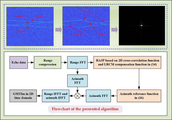
3. Proposed Algorithm Description

As analyzed in Section 2.2, the RCM, DCS, DFB, and Doppler ambiguity are the critical problems faced by the SAR-GMTIm. Therefore, a new approach is developed in this section to deal with these critical problems and obtain an effective focusing result. Figure 4 depicts the flowchart of the developed GMTIm method. On the basis of Figure 4, the proposed GMTIm approach is described in the following.
Initially, the signal in Equation (5) is transformed into the range-frequency and the azimuth-time domain, and the corresponding result, omitting the azimuth window, is written as [13,14]:
s 1 ( f , t n ) = rect ( f B ) exp [ j 4 π c ( f + f c ) ( R 0 v c t n + ( v v a ) 2 2 R 0 t n 2 ) ] .
Based on Equation (8), a RAJP 2D cross-correlation function in the range-frequency and azimuth-time domain is constructed as:
s 2 ( f , t n ) = s 1 ( f , t n + η / 2 ) s 1 * ( f , t n η / 2 )       = rect ( f B ) exp [ j 4 π c ( f + f c ) ( v c η + ( v v a ) 2 η R 0 t n ) ]
where “ ” and η denote the conjugate operation and constant delay, respectively. Generally, the selection criteria of η refer to Appendix A. As shown in Equation (9), the quadratic phase of Equation (8) is reduced to the linear phase in the range-frequency and azimuth-time domain. Therefore, the QRCM and DFB are simultaneously removed due to RAJP. Then, the Doppler spectrum ambiguity is also avoided, given that the DFB is addressed. However, the effect of the t n -term in Equation (9) still remains. Thus, the LRCM of Equation (9) should be compensated further.
As demonstrated in previous work by the authors of [36,37], the LRCM of Equation (9) for the common meter-level range resolution SAR mainly depends on the velocity of the SAR platform because v is far larger than the along-track velocity v a . Therefore, a compensation function related to v can be proposed to remove the LRCM of Equation (9), as long as the correction error is smaller than one range bin. According to Equation (9), the LRCM compensation function can be presented as:
H 1 ( f , t n ) = exp [ j 4 π ( f + f c ) ϕ η c t n ]
where ϕ = v 2 / R 0 . When multiplying Equation (9) by Equation (10), the compensation error of Equation (10) can normally be ignored, given that the SAR platform velocity v is the main factor in determining the LRCM of Equation (9).
After removing LRCM, the signal in Equation (9) is rewritten as:
s 3 ( f , t n ) = rect ( f B ) exp [ j 4 π c ( f + f c ) v c η ] exp [ j 4 π λ φ η t n ]
where φ = [ ( v v a ) 2 / R 0 ] ϕ .
After the range IFFT and azimuth FFT are employed to Equation (11), we have:
s 3 ( t , f t n ) = s 3 ( f , t n ) exp ( j 2 π f t n t n ) exp ( j 2 π f t ) d t n d f = δ ( t + 2 v c η / c ) δ ( f t n + 2 φ η / λ )
where δ ( · ) is the Dirac delta function and f t n is the azimuth Doppler frequency variable with respect to t n .
As shown in Equation (12), the clear peak will appear at:
t = 2 v c η / c ,   f t n = 2 φ η / λ .
According to Equation (13), the proposed RAJP, based on the 2D cross-correlation function and LRCM compensation function, can be summarized as follows:
( t ^ , f ^ t n ) = Peak t , f t n | IFFT f { FFT t n [ s 1 ( f , t n + η / 2 ) s 1 * ( f , t n η / 2 ) H 1 ( f , t n ) ] } |
where FFT t n ( · ) represents the FFT operation along t n , IFFT f ( · ) denotes the IFFT operation along f , and Peak ( · ) indicates the operation of peak detection [13].
Then, on the basis of RJAP, the first-order phase μ 1 = v c and quadratic phase μ 2 , i.e., μ 2 = ( v v a ) 2 / ( 2 R 0 ) , are simultaneously obtained in the range-time and azimuth-frequency domain, as follows:
μ ^ 1 = c t ^ / ( 2 η ) ,   μ ^ 2 = λ f ^ t n / ( 4 η ) + v 2 / ( 2 R 0 ) .
According to Equations (12), (13) and (15), compared with the typical DPT-based method in [28], the proposed RAJP-based approach has the following advantages: (1) the presented approach does not ignore the influence of QRCM and avoids the search for the Doppler ambiguity number; (2) the proposed RAJP operation can simultaneously remove the couplings between range and azimuth and between first- and second-order phase parameters; (3) the first- and second-order phase parameters can be simultaneously obtained in the fast-time and azimuth-frequency domains. Therefore, the propagation error from obtaining parameters using the stepwise processing operation can be avoided.
On the basis of the obtained parameters in Equation (15), the azimuth reference function in the range-frequency and azimuth-time domain is constructed as:
H 2 ( f , t n ) = exp { j 4 π ( f + f c ) c [ c t ^ 2 η t n + ( λ f ^ t n 4 η + v 2 2 R 0 ) t n 2 ] } .
Then, the azimuth-matched operation in the range- and azimuth-frequency domains can be summarized as follows:
s 4 ( f , f t n ) = [   s 1 ( f , t n ) exp ( j 2 π f t n t n ) d t n ] · [   H 2 ( f , t n ) exp ( j 2 π f t n t n ) d t n ] .
After the range IFFT and azimuth IFFT are applied to Equation (17), the result of GMTIm in the 2D time domain is obtained as:
s 5 ( t , t n ) = sin c [ B ( t 2 R 0 / c ) ] · sin c ( f d t n )
where f d indicates the Doppler bandwidth of the moving target.
As described in Equation (18), the effects of RCM, DCS, and DFB can be accurately eliminated, and a well-focused result can be achieved within the 2D time domain. Therefore, unlike the conventional GMTIm method [8,9,13,15,19,26], which focuses on the moving targets in the range–Doppler domain, the moving targets are focused in the range–azimuth time domain using the proposed method, thereby facilitating the subsequent processing operations of moving targets [23].

4. Some Discussions of the Proposed Method

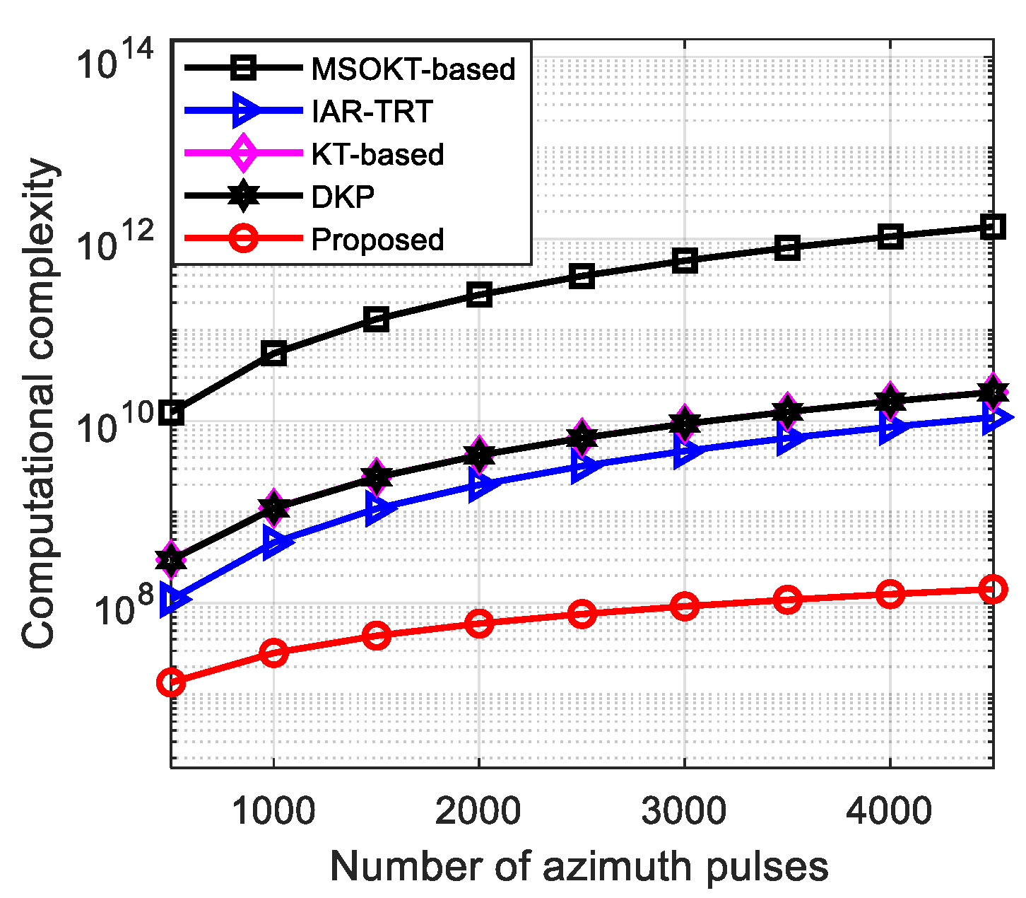
4.1. Analysis Related to Computational Complexity

In the following section, the computational burden of the developed approach is analyzed. Similar to [9,13], the complex multiplication numbers are applied to denote the computational complexity of the algorithm. The range and azimuth cell numbers are represented by M and N , respectively. The main steps of the developed approach contain the proposed RAJP, based on the 2D cross-correlation function, LRCM compensation function, and azimuth-matched operation. The main computational complexity of the proposed RAJP, based on the 2D cross-correlation function and LRCM compensation function, is obtained using O ( N M log 2 M + M N log 2 N ) . Then, the main computational cost of the azimuth-matched operation is represented by O ( N M log 2 M + M N log 2 N ) . Therefore, the main computational burden of the developed approach is denoted using O ( 2 N M log 2 M + 2 M N log 2 N ) . We assume that the searching times for the Doppler ambiguity number and the MSOKT-based and IAR-TRT methods are indicated by N d , N 1 , and N 2 . With regard to the MSOKT-based method, the main computational cost is indicated by O [ ( N 1 + 1 ) N M log 2 N ] [13]. In the IAR-TRT method, the main computational complexity is obtained using O [ ( N 2 + 4 ) N M log 2 N ] [9]. Then, the main computational cost for the DKP method is O [ M N 2 + N ( N 1 ) M + ( N d + 1 ) ( N M log 2 M + M N log 2 N ) ] [15]. According to the authors of [26], the main computational cost of the KT-based method is obtained using O [ M N 2 + N ( N 1 ) M + N d ( N M + N M log 2 M + M N log 2 N ) ] . The detailed computational costs of the five approaches are shown in Table 1. The curves of the computational costs versus the azimuth cell number with these five approaches are shown in Figure 5. The results of Table 1 and Figure 5 prove that the computational burdens of the IAR–TRT, MSOKT-based, DKP, and KT-based approaches are obviously higher than that of the developed approach. Furthermore, the developed approach offers high computational efficiency because it does not include the target parameter-searching procedure and can simultaneously obtain the first- and second-order parameters in the fast-time and azimuth-frequency domains, while needing fewer processing steps.

4.2. Analysis Related to a Mismatch of the LRM Compensation Function

In Section 3, the compensation function in Equation (10), constructed from the velocity of the SAR platform, is adopted to remove the LRCM of Equation (9). However, in some high-range-resolution SAR systems, the compensation error Δ R LRCM of Equation (9) may be larger than one range cell. In this case, the residual correction error Δ R LRCM after performing the compensation function in Equation (10) should be eliminated further. As described in Equations (9)–(11), the residual correction error Δ R LRCM induced by the t n -term coefficient φ η is a form of typical LRCM.
Some typical approaches, for example, the radon transform [17], Hough transform [16,37] and radon Fourier transform [38] have been suggested to remove the LRCM. Therefore, these typical approaches can also be adopted to eliminate the residual correction error Δ R LRCM . However, as in the parameter-searching-based approaches, the radon, radon Fourier and Hough transforms are computationally prohibitive, given the brute-force parameter search steps. On the other hand, the Keystone transform suffers from the problem of Doppler ambiguity. Therefore, in the following part, according to the geometric features of residual correction error (i.e., residual LRCM ) in the range- and azimuth-time domains, an operation based on the PCA technique is introduced to correct the residual correction error Δ R LRCM .
Then, the geometric features of the residual correction error are analyzed. Figure 6 shows the diagram of geometric features for residual correction error in the range- and azimuth-time domains. As exhibited in Figure 6, the residual correction error is the linear trajectory. β indicates the included angle between the trajectory and the slow time axis. Δ t n = P R F · Δ t m denotes the length of a discrete slow time for the trajectory of the residual correction error. Δ t m is the length of slow time after applying the 2D cross-correlation function in Equation (9).
According to Figure 6, the slope of the linear trajectory for the residual correction error (i.e., tan ( β ) ) can be written as follows:
tan ( β ) = Δ R LRCM Δ t n = Δ R LRCM P R F · Δ t m .
On the basis of Equation (11), Δ R LRCM is obtained as follows: Δ R LRCM = 2 φ η Δ t m f r / c , where f r denotes the range-sampling frequency. Then, tan ( β ) in Equation (19) can be rewritten as:
tan ( β ) = 2 φ η f r P R F · c   .
According to Equation (20), we have:
φ = tan ( β ) · P R F · c 2 η f r   .
Therefore, in accordance with Equation (21), to obtain the unknown coefficient φ , the slope tan ( β ) should be obtained first. The IAR method employed by the authors of [18] can be adopted to obtain the slope of the target trajectory. However, the IAR method suffers from a huge computational cost because it involves a parameter-search operation. Therefore, an operation using the PCA technique is applied to obtain the slope of the target trajectory.
The PCA technique usually maps the given data set into a new coordinate system and is adopted to confirm the maximum variance direction of the data set [39]. First, the first coordinate of the new coordinate system denotes the largest variance of the given data set. The largest variance is indicated by the first principal component in the PCA method. Then, the main energy of the direction of the given data set is then confirmed. Therefore, the PCA technique is applied to determine the main energy direction of LRCM for the given data set in the following part.
First, the database D to be processed is normalized, as follows:
D n = D max ( D )
where D n indicates the normalized form of D , and max ( · ) denotes the operation of obtaining the matrix maximum element value. The positions of strong points for the LRCM trajectories should be extracted by utilizing the set threshold. In order to obtain the strong point positions comprehensively in this study, the threshold is generally set as 0.5 [40]. On the basis of the set threshold, the database D e for the positions of the extracted data points is formed, as follows:
D e = [ D e 1 , , D e k ]
where D e k = [ n r k , n a k ] T represents the coordinate of the kth extracted data point in the range and azimuth dimension, while k denotes the number of extracted data points.
Then, the new data matrix D ^ e is obtained as:
D ^ e = D e D ¯ e
where D ¯ e = [ N r , N a ] T is the mean vector of D e , N r = 1 K k = 1 K n r k , and N a = 1 K k = 1 K n a k .
The covariance matrix with D ^ e is constructed as follows:
C c = 1 K ( D ^ e ) ( D ^ e ) T ,
Notably, C c is the real symmetric matrix. Therefore, the eigenvalue decomposition of C c is denoted as follows:
C c = P P T
where is the diagonal matrix, which has two eigenvalues, and P indicates the eigenvalues related to . Therefore, the eigenvector ( n r , n a ) for the largest eigenvalue is the direction of the principal axis. Then, the slope of the trajectory of LRCM is calculated as follows:
tan ( β ) = n r / n a
On the basis of Equations (21) and (27), the first-order coefficient is obtained as:
φ ^ = n r · P R F · c 2 · η · f r · n a
In accordance with Equation (26), the residual LRCM compensation function is constructed as follows:
H 2 ( f , t n ) = exp ( j 4 π f c n r · P R F · c 2 · f r · n a t n )
Therefore, after the compensation function in Equation (29) is adopted, the residual LRCM can be effectively removed.
Here, a simulation example, denoted as Example A, is provided to verify the above analysis for the mismatch of the LRCM compensation function. The main simulated parameters for the radar are set as follows: f c = 10 GHz, B = 400 MHz, P R F = 600 Hz, R 0 = −13 km and T a = 2 s. The moving target, with v c = 11.5 m/s and v a = −20.6 m/s is set. The signal-to-noise ratio (SNR) in this example is set as −12 dB. Figure 7 shows the simulated results of Example A. The clear LRCM is shown in Figure 7a, given that the residual correction error is larger than one range cell and it cannot be ignored. Figure 7b displays the final result of the proposed RJAP in Equation (14). The target energy still spreads along the fast time dimension. As shown in Figure 7c, the residual correction error can be removed effectively by the PCA-based operation, and the target energy is located in one range cell. Figure 7d plots the final result of the proposed RJAP in Equation (14) and a PCA-based operation. The peak is evident in Figure 7d. Therefore, the above results can verify the performance of the PCA-based operation.

4.3. Analysis Related to Multiple Target Focusing

According to Section 3, the results of GMTIm for a single target can be effectively obtained by the developed method. However, the multiple moving targets may be available in the SAR scene. The cross-terms induced by multiple targets should be further investigated. As for the case of multiple targets, the signals in Equation (8) are written as follows:
s 1 , m ( f , t n ) = l = 1 G rect ( f B ) exp [ j 4 π c ( f + f c ) ( R 0 , l + μ 1 , l t n + μ 2 , l t n 2 ) ]
where R 0 , l denotes the nearest slant range of the l th moving target. μ 1 , l = v c , l and μ 2 , l = ( v v a , l ) 2 / ( 2 R 0 , l ) indicate the first- and second-order range coefficients of the l th target.
After compensating for RCM and DFB, the corresponding signal of the multiple target case is expressed as:
s 3 , m ( f , t n ) = l = 1 G rect ( f B ) exp ( j 4 π λ φ 2 , l η t n ) exp ( j 4 π c ( f + f c ) μ 1 , l η ) auto terms       + l = 1 G d = 1 , d l G rect ( f B )       × exp { j 4 π λ φ 2 , l , d η t n } exp [ j 4 π c ( f + f c ) ( R 0 , l R 0 , d ) ]       × exp { j 4 π c ( f + f c ) [ ( μ 1 , l μ 1 , d ) t n + ( μ 2 , l μ 2 , d ) t n 2 ] }       × exp { j 4 π c ( f + f c ) [ ( μ 1 , l + μ 1 , d ) η 2 + ( μ 2 , l μ 2 , d ) η 2 4 ] } cross terms
where φ 2 , l , d = ( μ 2 , l + μ 2 , d ) ϕ . After the range IFFT and azimuth FFT are applied to (31), we obtain:
s 3 , m ( t , t n ) = l = 1 G sin c [ B ( t μ 1 , l η c ) ] exp ( j 4 π λ φ 2 , l η t n ) auto   terms + l = 1 G d = 1 , d l G exp [ j 4 π λ ( μ 1 , l μ 1 , d + φ 2 , l , d η ) t n + ( μ 2 , l μ 2 , d ) t n 2 ] × sin c { B [ t R 0 , l R 0 , d + ( μ 1 , l + μ 1 , d ) η 2 + ( μ 2 , l μ 2 , d ) η 2 4 + ( μ 1 , l μ 1 , d ) t n + ( μ 2 , l μ 2 , d ) t n 2 c ] } cross   terms
According to (32), the RCMs and DFBs of the auto terms are removed, and only the linear phase remains. The auto terms can be identified as clear peaks after performing the azimuth FFT. Considering that the RCMs and DFBs of the cross-terms still exist, the cross-terms are typically defocused. Therefore, the cross terms may not affect the determination of the auto terms.

4.4. Remarks

Remark 1.
The different moving target signals may have various amplitudes. When the intensities of these moving target signals are obviously different, the moving target with a lower intensity may be drowned out by the one with a higher intensity. This factor will reduce the performance of the developed approach. In this situation, the CLEAN technique [40,41] can be adopted to eliminate the effect of the moving target with a higher intensity. Then, the focused results of the strong and weak moving targets can be obtained iteratively.
Remark 2.
In some applications, such as focusing on highly mobile targets, the high-order motion model should be considered. With respect to highly mobile targets with high-order motions, the high-order (more than the second-order) range model may be appropriate. In this situation, the range-compressed signal in Equation (8) should be rewritten as follows:
s 1 ( f , t n ) = rect ( f B ) exp [ j 4 π c ( f + f c ) ( R 0 + μ 1 t n + μ 2 t n 2 ) ] × exp [ j 4 π c ( f + f c ) ( d = 3 D μ d t n d ) ]
where d denotes the order of the high-order phase coefficient.
In order to extend the above-proposed method and adapt it to process the high-order (more than the second-order) phase of a maneuvering target, another search phase function, based on the target’s high-order range model, is constructed as follows:
H h m ( f , t n ; μ ^ 3 , , μ ^ d ) = exp [ j 4 π c ( f + f c ) ( d = 3 D μ ^ d t n d ) ]
where μ ^ d ( d = 3 , D ) denotes the d -th search phase parameter.
After multiplying Equation (34) by Equation (33), this yields:
s 1 ( f , t n ; μ ^ 3 , , μ ^ d ) = s 1 ( f , t n ) H h m ( f , t n ; μ ^ 3 , , μ ^ d ) = rect ( f B ) exp [ j 4 π c ( f + f c ) ( R 0 + μ 1 t n + μ 2 t n 2 ) ] × exp [ j 4 π c ( f + f c ) [ d = 3 D ( μ d μ ^ d ) t n d ] ]
When the searching parameters are matched with the true value of the target’s phase parameters (i.e., μ d = μ ^ d ), Equation (35) can be simplified as follows:
s m ( f , t n ) = rect ( f B ) exp [ j 4 π c ( f + f c ) ( R 0 + μ 1 t n + μ 2 t n 2 ) ]
As shown in Equation (36), after the matched processing in Equation (35), the above-developed method can be applied to process the signal in Equation (36). Therefore, according to the above-proposed method, the procedure of estimating the high-order phase parameters can be summarized as follows:
( μ ^ 3 , , μ ^ d ) = argmax | IFFT f { FFT t n [ s 1 ( f , t n + η 2 ; μ ^ 3 , , μ ^ d ) × s 1 * ( f , t n η 2 ; μ ^ 3 , , μ ^ d ) H 1 ( f , t n ) ] } |
In accordance with the estimated high-order phase parameters from Equation (37), the defocusing of the high-order phase can be compensated for. Therefore, after using the pre-processing steps in Equation (37) for high-order parameter estimation, the proposed method in Section 3 can be extended for high-order focusing.
However, this pre-procedure increases the computational complexity. Therefore, the computationally efficient method for focusing on a maneuvering target with a high-order (more than second-order) phase model will be investigated in future work.

5. Experiment Results

In the following section, the simulated data in the presence of a Gaussian background and the measured data (including spaceborne and airborne measured data) are processed to verify the performance of the developed approach for the imaging of ground-based moving targets.

5.1. Simulated Experimental Results Analysis

In this simulation experiment, the basic simulated parameters of radar are provided in Table 2. Three moving targets are considered, and these are denoted as Targets A, B, and C. The main parameters of these three simulated moving targets are given in Table 3. The SNR in this simulated experiment is the same as in Example A. Target A and Target B are Doppler spectrum ambiguity targets. The Doppler spectra of Target A and Target B are split into two adjacent PRF bands, and their spectrum distributions are similar to Case 2 in Figure 2b. Target C is set as a Doppler center blur target. The Target C’s Doppler spectrum is entirely distributed in one PRF band, and its spectrum distribution is similar to that in Case 1 in Figure 2a.
The simulated data-processed results are provided in Figure 8. The three curved trajectories of Target A, Target B, and Target C after range compression are shown in Figure 8a, from which the three curved trajectories indicate evident RCMs (including the LRCMs and QRCMs) of the moving targets. The RCMs make the moving target energy spread along the range dimension, thereby leading to the defocusing of the moving target in the range dimension. The Doppler spectra of three moving targets in the range-time and the Doppler-frequency domain are displayed in Figure 8b. Notably, the target energy still distributes into several azimuth Doppler cells because of the influence of DFB, thereby inducing the defocusing of the moving target in the azimuth Doppler dimension. In addition, the Doppler spectra of Target A and Target B span over two adjacent PRF bands, and the Doppler spectrum of Target C entirely occupies one PRF band. The complex Doppler spectrum distribution results in problems with the imaging of moving targets. Figure 8c illustrates the results of RAJP based on the 2D cross-correlation function and the LRCM compensation function. As shown in Figure 8c, the RCMs and DFBs are simultaneously removed and three clear peaks, with respect to Target A, Target B, and Target C, are found in the figure. Then, in order to display the cross-terms clearly, the background is migrated. The corresponding result is indicated in Figure 8d. As shown in the figure, with regard to the cross-terms, the influences of both the first- and second-order phases (i.e., LRCM, QRCM, and DFB) remain. Therefore, the cross-terms still suffer from the effects of defocusing, which helps us to reject the cross-terms. In this case, the cross-terms do not affect the auto terms. Notably, the first- and second-order phase parameters of the moving targets can simultaneously be obtained by the peak positions in the fast-time and azimuth-frequency domains with a low computational cost, which can avoid the propagation error caused by stepwise parameter estimation. With the obtained phase parameters from the peaks in Figure 8c, the corresponding azimuth reference functions, with respect to Target A, Target B, and Target C, are constructed. On the basis of the constructed azimuth reference functions, Target A, Target B, and Target C are focused in the range- and azimuth-time. As shown in Figure 8e–j, respectively, the clearly imaged results of Target A, Target B, and Target C can be achieved by using the developed approach. Figure 8k shows the processing result of the KT-based method. The motion trajectories of Target A and Target B divide into several parts because the Keystone is directly utilized to remove the RCM for the KT-based approach in the presence of Doppler spectrum splitting, which will result in a serious loss of coherent integration and reduce the imaging performance. The focusing result of Target B for the MSOKT-based method is provided in Figure 8l. As shown in the figure, this method suffers from the effect of BSSL, given that its implementation steps include the search operation of the first-order phase. Figure 8m shows the result for Target B for the DKP approach. The focusing performance of the DKP approach deteriorates markedly because the effect induced by the unknown motion of the moving target is neglected.
To summarize, the presented method can simultaneously obtain the first- and second-order phase parameters of moving targets in the fast-time and azimuth-frequency domains without suffering the propagation error induced by the operation of the stepwise parameter estimation. The proposed approach can produce a well-focused result without the residual correction errors induced by the unknown motions of the moving targets. In addition, the presented algorithm can deal with the effect of BSSL and is also robust when faced with Doppler ambiguity (containing a complex Doppler center blur and spectrum ambiguity).

5.2. Spaceborne Real Data Result Analysis

In this subsection, two C-band spaceborne data segments collected by the RADARSAT-1 system, which contains a single target or two targets, are processed to verify the performance of the developed approach. The basic radar parameters are provided in Table 4. The detailed parameters of these spaceborne measured data are taken from [1].
Figure 9a gives an example showing the data for a single target, where the selected moving target is marked with a red oval box in the figure. Figure 9b plots the trajectory of the selected target after performing the range compression procedure. As shown in Figure 9b, the curved trajectory of the moving target spans several range cells, given the severe effect of RCM, which makes the target energy spread along the range dimension and shows typical defocusing. Then, the RJAP, based on the 2D cross-correlation function and LRCM compensation function in Equation (14), is applied to process the selected target. The corresponding result is displayed in Figure 9c. The RCM and DFB of the selected target are simultaneously eliminated and an evident peak corresponding to the selected target is shown in Figure 9c. With the target peak position set, the corresponding azimuth reference function is constructed to focus on the selected target. As exhibited in Figure 9d, a well-focused result can be achieved using the proposed method. Then, the processing results from adopting the MSOKT-based [13] and IAR-TRT [9] methods are presented for comparison. Figure 9e indicates the processing result of the MSOKT-based method. As exhibited in Figure 9e, the MSOKT-based method suffers from a serious BSSL problem. The processing results of the IAR-TRT method are shown in Figure 9f–h. As shown in Figure 9g, the estimation of the second-order phase is invalid, given that the IAR-TRT method suffers from a severe problem of scaled frequency spectrum aliasing. Therefore, the focusing performance of the IAR-TRT approach degrades significantly, as shown in Figure 9h. In summary, the above-obtained results verify the performance of the proposed approach. In comparison with the MSOKT-based method, the problem of BSSL can be addressed by adopting the presented approach. Compared with the IAR-TRT method, the developed method has good imaging performance, given that the scaled frequency spectrum aliasing is avoided.

5.3. Airborne Real Data Results Analysis

In this part, a segment of airborne SAR data, which is measured by an X-band three-channel radar system with the working model of a side-facing strip-map, is processed to validate the effectiveness of the proposed method. The velocity of the radar moving platform is 120 m/s.
Figure 10a shows the image of the selected airborne data in the range-Doppler domain after range compression. The moving targets are submerged in the severe ground clutter. Then, the extended factored approach [42] is adopted to suppress the serious ground clutter. The result of the clutter cancellation is provided in Figure 10b. The target of interest, indicated by Target 1, is marked with a red rectangular box in Figure 10b.
The trajectory of Target 1 in the range-Doppler domain is displayed in Figure 10c. As shown in the figure, the target trajectory indicates the typical defocusing in the range-Doppler domain. Then, the RJAP, based on the 2D cross-correlation function and LRCM compensation function in Equation (14), is performed for the processing of Target 1, and the processing result is plotted in Figure 10d. On the basis of the clear peak with respect to Target 1 in Figure 10d, the corresponding azimuth reference function is constructed to create an image of Target 1. As shown in Figure 10e, the focused result is obtained by using the proposed method. Figure 10f displays the focusing result of the DKP method [15] for Target 1.
As plotted in Figure 10f, Target 1 is still defocused, given that the DKP method neglects the effect of target motion (i.e., along-track velocity). Therefore, the above-mentioned processing results of the airborne real data confirm the effectiveness of the proposed approach. Compared with the DKP method, the presented approach has good focusing performance because the effect of the along-track velocity of a moving target is taken into account.

6. Conclusions

The RCM and DFB caused by the unknown relative motions between the radar unit and a non-cooperative target are the main factors causing the defocusing of moving targets. Additionally, the Doppler ambiguity leads to difficulties in the correction of RCM and DFB. In order to deal with these issues, a rapid approach based on RAJP is proposed for the SAR imaging of ground-based moving targets. The main properties of the proposed approach are summarized as follows: (1) the RAJP operation is proposed to simultaneously decouple the couplings between the range and azimuth and between the first- and second-order parameters; this can simplify the processing steps for moving-target imaging; (2) the first- and second-order phase parameters can simultaneously be obtained in the fast-time and azimuth-frequency domains by using the proposed approach, which bypasses the propagation error induced by the operation of the stepwise parameter estimation; (3) the proposed algorithm has high computational efficiency, given fewer processing steps; (4) the developed approach can address the problems of complex Doppler ambiguity and BSSL; (5) on the basis of this analysis corresponding to the mismatch of the LRCM compensation function, the PCA-based approach is introduced to address the LRCM compensation function mismatch.
However, the proposed method is suitable for the fast imaging of the uniform moving target with the second-order model with a homogeneous background. Therefore, the computationally efficient method for imaging a target with a high-order (more than second-order) range model and imaging a moving target with a heterogeneous background will be investigated in the future.

Author Contributions

Conceptualization, Y.S., J.W. and D.L.; data curation, Y.S. and J.W.; formal analysis, Y.S. and J.W.; funding acquisition, J.W., Z.C., Y.S. and D.L.; investigation, Y.S.; methodology, Y.S., J.W. and D.L.; project administration, D.L. and H.L.; supervision, D.L. and H.L.; validation, Y.S., J.W. and D.L.; writing—original draft, Y.S.; writing—review and editing, J.W., Z.C., D.L. and H.L. All authors have read and agreed to the published version of the manuscript.

Funding

This research was funded by the Engineering Research Center of Mobile Communications, Ministry of Education, under Grant cqupt-mct-202103; the Natural Science Foundation of Chongqing, China under Grant cstc2021jcyj-bshX0085; the Opening Project of the Guangxi Wireless Broadband Communication and Signal Processing Key Laboratory, under Grant GXKL06200214 and Grant GXKL06200205; the National Natural Science Foundation of China, under Grant 61971075, Grant 62001062, and Grant U20A20157; the Key Project of the Application and Development of Chongqing, under Grant cstc2019jscx-fxydX0049.

Data Availability Statement

Data sharing is not applicable to this article.

Conflicts of Interest

The authors declare no conflict of interest.

Appendix A

In this Appendix, the selection criterion of the constant delay η in the developed approach is discussed.
According to Equation (12), if the true first- and second-order phase parameters of the moving target signal cannot be indicated by the integer multiple resolutions in the fast-time and azimuth-frequency domains, the maximum estimation error of the phase parameters is less than one resolution cell. Therefore, the estimation errors of the first- and second-order phase parameters (i.e., Δ μ ^ 1 and Δ μ ^ 2 ) are written as follows:
Δ μ ^ 1 = c Δ t / ( 2 η ) , Δ μ ^ 2 = λ Δ f t n / ( 4 η )
where Δ t = 1 / ( 2 f r ) denotes the resolution of the fast-time dimension of Equation (12), and Δ f t n = 1 / { T i [ η / 2 ( η / 2 ) ] } indicates the resolution of the azimuth-frequency dimension of Equation (12).
Then, Equation (A1) can be rewritten as follows:
Δ μ ^ 1 = c / ( 4 η f r ) , Δ μ ^ 2 = λ / [ 4 η ( T i η ) ] .
Thereafter, Equation (A2) is equivalently presented as:
Δ μ ^ 1 = c / ( 4 η f r ) , Δ μ ^ 2 = λ / [ 4 ( η T i / 2 ) 2 + T i 2 ] .
According to Equation (A3), the estimation error of the first-order phase parameter (i.e., Δ μ ^ 1 ) is inversely proportional to η . Therefore, if a large value for η is selected, the estimation error Δ μ ^ 1 will be reduced. Then, the performance of the estimation of the first-order phase parameter will improve. However, η increases with the decline in the integration pulse number for Equation (12), which causes the coherent cumulative gain in Equation (12) to decrease. Hence, regarding the estimation of μ 1 , the selection value of η needs to achieve a good balance between the coherent cumulative gain in Equation (12) and parameter estimation accuracy. On the other hand, according to Equation (A3), when η = T i / 2 , the estimation error of the second-order phase parameter (i.e., Δ μ ^ 2 ) can obtain the minimum value. Therefore, regarding the estimation of   μ 2 , the η = T i / 2 is the optimal selection value. In summary, according to the above-mentioned analysis, considering the estimation accuracies of   μ 1 and   μ 2 and coherent cumulative gain, η is recommended to be selected as T i / 2 in this work.

References

  1. Cumming, I.G.; Wong, F.H. Digital Processing of Synthetic Aperture Radar Data: Algorithm and Implementation; Artech House: Norwood, MA, USA, 2005. [Google Scholar]
  2. Moreira, A.; Iraola, P.P.; Younis, M.; Krieger, G.; Hajnsek, I.; Papathanassiou, K.P. A tutorial on synthetic aperture radar. IEEE Geosci. Remote Sens. Mag. 2013, 1, 6–43. [Google Scholar] [CrossRef] [Green Version]
  3. Alver, M.B.; Saleem, A.; Cetin, M. Plug-and-play synthetic aperture radar image formation using deep priors. IEEE Trans. Comput. Imag. 2021, 7, 43–57. [Google Scholar] [CrossRef]
  4. Liu, N.; Ge, G.; Tang, S.; Zhang, L. Signal modeling and analysis for elevation frequency scanning HRWS SAR. IEEE Trans. Geosci. Remote Sens. 2020, 58, 6434–6450. [Google Scholar]
  5. Pu, W.; Wu, J. OSRanP: A novel way for radar imaging utilizing joint sparsity and low-rankness. IEEE Trans. Comput. Imag. 2020, 6, 868–882. [Google Scholar]
  6. Tang, S.; Guo, P.; Zhang, L.; So, H.C. Focusing hypersonic vehicle-borne SAR data using radius/angle algorithm. IEEE Trans. Geosci. Remote Sens. 2020, 58, 281–293. [Google Scholar] [CrossRef]
  7. Huang, Y.; Liao, G.; Xu, J.; Li, J.; Yang, D. GMTI and parameter estimation for MIMO SAR system via fast interferometry RPCA method. IEEE Trans. Geosci. Remote Sens. 2018, 56, 1774–1787. [Google Scholar] [CrossRef]
  8. Wan, J.; Chen, Z.; Zhou, Y.; Li, D.; Huang, Y.; Zhang, L. Ground moving target imaging based on MSOKT and KT for synthetic aperture radar. In Proceedings of the 2020 IEEE International Geoscience and Remote Sensing Symposium, Virtual Symposium, 26 September–2 October 2020; pp. 2141–2144. [Google Scholar]
  9. Huang, P.; Xia, X.G.; Liu, X.; Liao, G. Refocusing and motion parameter estimation for ground moving targets based on improved axis rotation-time reversal transform. IEEE Trans. Comput. Imag. 2018, 4, 479–494. [Google Scholar] [CrossRef]
  10. Baumgartner, S.V.; Krieger, G. Simultaneous high-resolution wide-swath SAR imaging and ground moving target indication: Processing approaches and system concepts. IEEE J. Sel. Topics Appl. Earth Observ. Remote Sens. 2015, 8, 5015–45029. [Google Scholar] [CrossRef]
  11. Chen, Z.; Zhou, S.; Wang, X.; Huang, Y.; Wan, J.; Li, D.; Tan, X. Single range data-based clutter suppression method for multichannel SAR. IEEE Geosci. Remote Sens. Lett. 2022, 19, 4012905. [Google Scholar] [CrossRef]
  12. Dong, Q.; Xing, M.; Xia, X.; Zhang, S.; Sun, G. Moving target refocusing algorithm in 2-D wavenumber domain after BP integral. IEEE Geosci. Remote Sens. Lett. 2018, 15, 127–131. [Google Scholar] [CrossRef]
  13. Wan, J.; Zhou, Y.; Zhang, L.; Chen, Z. Ground moving target focusing and motion parameter estimation method via MSOKT for synthetic aperture radar. IET Signal Process. 2019, 13, 528–537. [Google Scholar] [CrossRef]
  14. Zhu, S.; Liao, G.; Qu, Y.; Zhou, Z.; Liu, X. Ground moving targets imaging algorithm for synthetic aperture radar. IEEE Trans. Geosci. Remote Sens. 2011, 49, 462–477. [Google Scholar]
  15. Sun, G.; Xing, M.; Xia, X.G.; Wu, Y.; Bao, Z. Robust ground moving-target imaging using deramp-Keystone processing. IEEE Trans. Geosci. Remote Sens. 2013, 51, 966–982. [Google Scholar] [CrossRef]
  16. Oveis, A.H.; Sebt, M.A. Coherent method for ground-moving target indication and velocity estimation using Hough transform. IET Radar Sonar Navig. 2017, 11, 646–655. [Google Scholar] [CrossRef]
  17. Moya, J.C.; Menoyo, J.G.; Lopez, A.A. Application of the radon transform to detect small-targets in sea clutter. IET Radar Sonar Navig. 2009, 3, 155–166. [Google Scholar] [CrossRef]
  18. Rao, X.; Zhong, T.; Tao, H.; Xie, J.; Su, J. Improved axis rotation MTD algorithm and its analysis. Multidim. Syst. Sign. Process. 2019, 30, 885–902. [Google Scholar] [CrossRef]
  19. Perry, R.P.; DiPietro, R.C.; Fante, R.L. SAR imaging of moving targets. IEEE Trans. Aerosp. Electron. Syst. 1999, 35, 188–200. [Google Scholar] [CrossRef]
  20. Zhu, D.; Li, Y.; Zhu, Z. A keystone transform without interpolation for SAR ground moving-target imaging. IEEE Geosci. Remote Sens. Lett. 2007, 4, 18–22. [Google Scholar] [CrossRef]
  21. Dai, Z.; Zhang, X.; Fang, H.; Bai, Y. High accuracy velocity measurement based on keystone transform using entropy minimization. Chin. J. Electron. 2016, 25, 774–778. [Google Scholar] [CrossRef]
  22. Kirkland, D. Imaging moving targets using the second-order keystone transform. IET Radar Sonar Navig. 2011, 5, 902–910. [Google Scholar] [CrossRef]
  23. Zhou, F.; Wu, R.; Xing, M. Approach for single channel SAR ground moving target imaging and motion parameter estimation. IET Radar Sonar Navig. 2007, 1, 59–66. [Google Scholar] [CrossRef]
  24. Li, G.; Xia, X.G.; Peng, Y. Doppler keystone transform: An approach suitable for parallel implementation of SAR moving target imaging. IEEE Geosci. Remote Sens. Lett. 2008, 5, 573–577. [Google Scholar] [CrossRef]
  25. Wan, J.; Tan, X.; Chen, Z.; Li, D.; Liu, Q.; Zhou, Y.; Zhang, L. Refocusing of ground moving targets with Doppler ambiguity using Keystone transform and modified second-order Keystone transform for synthetic aperture radar. Remote Sens. 2021, 13, 177. [Google Scholar] [CrossRef]
  26. Huang, P.; Liao, G.; Yang, Z.; Xia, X.G.; Ma, J.; Zhang, X. An approach for refocusing of ground moving target without motion parameter estimation. IEEE Trans. Geosci. Remote Sens. 2017, 55, 336–350. [Google Scholar] [CrossRef]
  27. Tian, J.; Cui, W.; Xia, X.G.; Wu, S. Parameter estimation of ground moving targets based on SKT-DLVT processing. IEEE Trans. Comput. Imag. 2016, 2, 13–26. [Google Scholar] [CrossRef] [Green Version]
  28. Pang, C.; Liu, S.; Han, Y. Coherent detection algorithm for radar maneuvering targets based on discrete polynomial-phase transform. IEEE J. Sel. Topics Appl. Earth Observ. Remote Sens. 2019, 12, 3412–3422. [Google Scholar] [CrossRef]
  29. Chen, X.; Guan, J.; Liu, N.; He, Y. Maneuvering target detection via Radon-fractional Fourier transform-based long-time coherent integration. IEEE Trans. Signal Process. 2014, 62, 939–953. [Google Scholar] [CrossRef]
  30. Li, X.; Sun, Z.; Yeo, T.S. Computational efficient refocusing and estimation method for radar moving target with unknown time information. IEEE Trans. Comput. Imag. 2016, 2, 13–26. [Google Scholar] [CrossRef]
  31. Wu, W.; Wang, G.; Sun, J. Polynomial radon-polynomial Fourier transform for near space hypersonic maneuvering target detection. IEEE Trans. Aerosp. Electron. Syst. 2018, 54, 1306–1322. [Google Scholar] [CrossRef]
  32. Zhan, M.; Huang, P.; Zhu, S.; Liu, X.; Liao, G.; Sheng, J.; Li, S. A modified keystone transform matched filtering method for space-moving target detection. IEEE Trans. Geosci. Remote Sens. 2022, 60, 1–16. [Google Scholar] [CrossRef]
  33. Lin, L.; Sun, G.; Cheng, Z.; He, Z. Long-time coherent integration for maneuvering target detection based on ITRT-MRFT. IEEE Sens. J. 2020, 20, 3718–3731. [Google Scholar] [CrossRef]
  34. Li, X.; Su, Z.; Yi, W.; Cui, G.; Kong, L. Radar detection and parameter estimation of high-speed target based on MART-LVT. IEEE Sens. J. 2019, 19, 1478–1486. [Google Scholar] [CrossRef]
  35. Sharif, M.R.; Abeysekera, S.S. Efficient wideband signal parameter estimation using a Radon-ambiguity transform slice. IEEE Trans. Aerosp. Electron. Syst. 2007, 43, 673–688. [Google Scholar] [CrossRef]
  36. Yang, J.; Liu, C.; Wang, Y. Detection and imaging of ground moving targets with real SAR data. IEEE Trans. Geosci. Remote Sens. 2015, 53, 920–930. [Google Scholar] [CrossRef]
  37. Tan, K.; Li, W. Imaging and parameter estimating for fast moving targets in airborne SAR. IEEE Trans. Comput. Imag. 2017, 32, 126–140. [Google Scholar] [CrossRef]
  38. Xu, J.; Yu, J.; Peng, Y.; Xia, X. Radon-Fourier transform for radar target detection I: Generalized Doppler filter bank. IEEE Trans. Aerosp. Electron. Syst. 2011, 47, 1186–1202. [Google Scholar] [CrossRef]
  39. Kang, M.-S.; Bae, J.-H.; Kang, B.-S.; Kim, K.-T. ISAR cross-range scaling using iterative processing via principal component analysis and bisection algorithm. IEEE Trans. Signal Process. 2016, 64, 3909–3918. [Google Scholar] [CrossRef]
  40. Misiurewicz, J.; Kulpa, K.S.; Czekala, Z.; Filipek, T.A. Radar detection of helicopters with application of CNEAN method. IEEE Trans. Aerosp. Electron. Syst. 2012, 48, 3525–3537. [Google Scholar] [CrossRef]
  41. Li, X.; Kong, L.; Cui, G.; Yi, W. CLEAN-based coherent integration method for high-speed multi-targets detection. IET Radar Sonar Navig. 2016, 10, 1671–1682. [Google Scholar] [CrossRef]
  42. DiPietro, R.C. Extended factored space–time processing for airborne radar systems. In Proceedings of the 26th Asilomar Conference on Signals, Systems, and Computers, Pacific Grove, CA, USA, 26–28 October 1992; pp. 425–430. [Google Scholar]
Figure 1. Motion geometric model between the SAR and moving target on the slant range plane.
Remotesensing 14 02965 g001
Figure 2. Potential Doppler spectrum distributions: (a) the Doppler spectrum, entirely distributed into one PRF band; (b) the Doppler spectrum, occupying two PRF bands; (c) the Doppler spectrum, spanning multiple PRF bands.
Remotesensing 14 02965 g002
Figure 3. Relationships among the target signal phase parameters, RCM, DFO, DCS, and DFB, and the Doppler ambiguity.
Remotesensing 14 02965 g003
Figure 4. Flowchart of the presented algorithm.
Remotesensing 14 02965 g004
Figure 5. Curves of the computational costs versus the azimuth cell number, with five approaches.
Remotesensing 14 02965 g005
Figure 6. Diagram of the geometric features for residual correction error in the range- and azimuth-time domains.
Remotesensing 14 02965 g006
Figure 7. Simulated results of Example A. (a) Trajectory after performing the proposed RJAP in Equation (14). (b) Final result of the proposed RJAP in Equation (14). (c) Trajectory after performing the proposed RJAP in Equation (14) and PCA-based operation. (d) Final result of the proposed RJAP in Equation (14) and the PCA-based operation.
Remotesensing 14 02965 g007
Figure 8. Simulated data and the processed results: (a) the results of three moving targets after range compression. (b) Doppler spectra of three moving targets. (c) The results of RJAP, based on the cross-correlation function and LRCM compensation function in Equation (14). (d) Plan of (c) without noise. (e) Focusing result of Target A, using the developed approach. (f) Stereogram of (e). (g) Focusing result of Target B, applying the proposed approach. (h) Stereogram of (g). (i) Focusing result of Target C, utilizing the proposed approach. (j) Stereogram of (i). (k) Processing result of Target B, adopting the KT-based method [26]. (l) Focusing result of Target B, using the MSOKT-based method [13]. (m) Focusing result of Target B, using the DKP approach [15].
Remotesensing 14 02965 g008aRemotesensing 14 02965 g008b
Figure 9. Spaceborne real data processing results for a single target. (a) Scene showing the requisite data for a single target. (b) The result of range compression for a single target. (c) The result of RJAP in Equation (14). (d) The focusing results of a single target by adopting the developed approach. (e) The focusing results of the MSOKT-based method [13]. (f) The output result of the IAR-TRT operation in [9]. (g) Result of the second-order phase estimation for the IAR-TRT method. (h) The focusing result of the IAR-TRT approach.
Remotesensing 14 02965 g009aRemotesensing 14 02965 g009b
Figure 10. Airborne measured data-processing results. (a) Scene of the selected airborne SAR data in the range-Doppler dimension. (b) Results after the grand clutter cancellation. (c) The trajectory of Target 1 in the range-Doppler domain. (d) The results of RJAP in Equation (14) for Target 1. (e) The focusing result of the proposed approach for Target 1. (f) The focusing result of the DKP method [15] for Target 1.
Remotesensing 14 02965 g010
Table 1. Comparison of the computational burden.
MethodsComputational Burden
MSOKT-based method O [ ( N 1 + 1 ) N M log 2 N ]
IAR-TRT method O [ ( N 2 + 4 ) N M log 2 N ]
DKP-based method O [ M N 2 + N ( N 1 ) M + ( N d + 1 ) ( N M log 2 M + M N log 2 N ) ]
KT-based method O [ M N 2 + N ( N 1 ) M + N d ( N M + N M log 2 M + M N log 2 N ) ]
Proposed method O ( 2 N M log 2 M + 2 M N log 2 N )
Table 2. Basic simulation radar parameters.
ParametersValue
Carrier frequency10 GHz
Range bandwidth80 MHz
Pulse repetition frequency600 Hz
Radar platform velocity180 m/s
Nearest slant range13 km
Dwell time2 s
Table 3. Simulation parameters for three moving targets.
Cross-Track Velocity (m/s)Along-Track Velocity (m/s)
Target A11.5−20.6
Target B22.4−15.2
Target C−16.7−12.5
Table 4. Basic parameters of C-band spaceborne radar.
ParametersValue
Carrier frequency5.3 GHz
Range bandwidth30.116 MHz
Pulse repetition frequency1256.98 Hz
Publisher’s Note: MDPI stays neutral with regard to jurisdictional claims in published maps and institutional affiliations.

