
Ant Colony Pheromone Mechanism-Based Passive Localization Using UAV Swarm


Abstract
:
1. Introduction
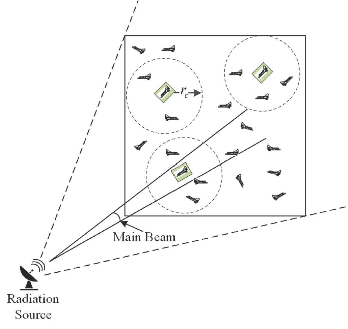
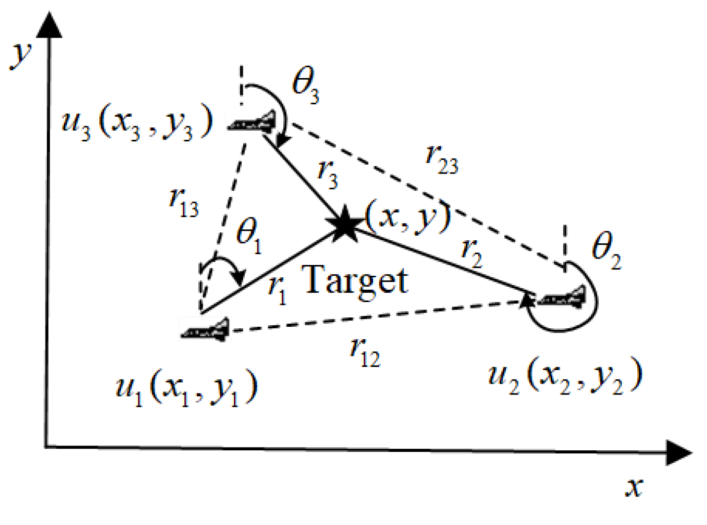
2. Problem Description and Modeling
3. The Proposed Method
3.1. Target Initial Position Estimate
3.2. The Ant Colony Pheromone Mechanism
| Algorithm 1 The pheromone update algorithm. |
| At time t, |
| Step1: Pheromone injection. Each UAV uses the current received target |
| bearing information to correct the initial position estimate . |
| 1:for |
| 2: if the i th UAV contains target position information |
| 3: |
| 6: End |
| 7:End |
| Step2: Pheromone transmission. Each UAV is weighted by the pheromone |
| transmitted by other UAVs in the communication radius |
| 1:for |
| 2: for |
| 3: if , and the j th UAV does not contain the |
| the target position pheromone |
| 4: |
| 5: else if the j th UAV contains the target position pheromone |
| 6: |
| 7: End |
| 8: End |
| 9:End |
3.2.1. Pheromone Injection
3.2.2. Pheromone Transmission
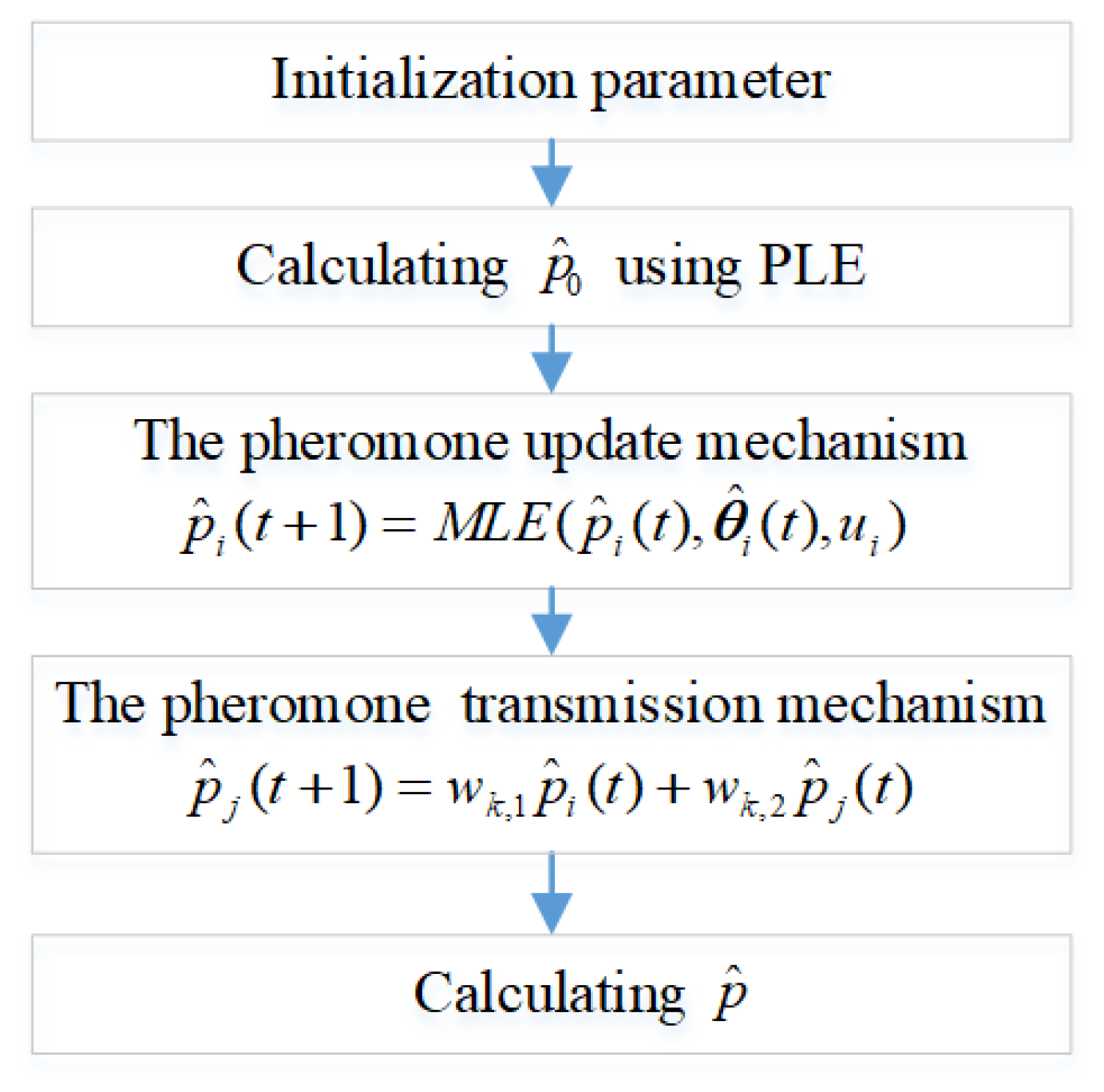
- (a)
- A small number of UAVs receiving radiation source signals use PLE to compute an initial target location estimate ;
- (b)
- Based on the pheromone injection mechanism, each UAV uses MLE to self-correct to obtain the next moment estimate ;
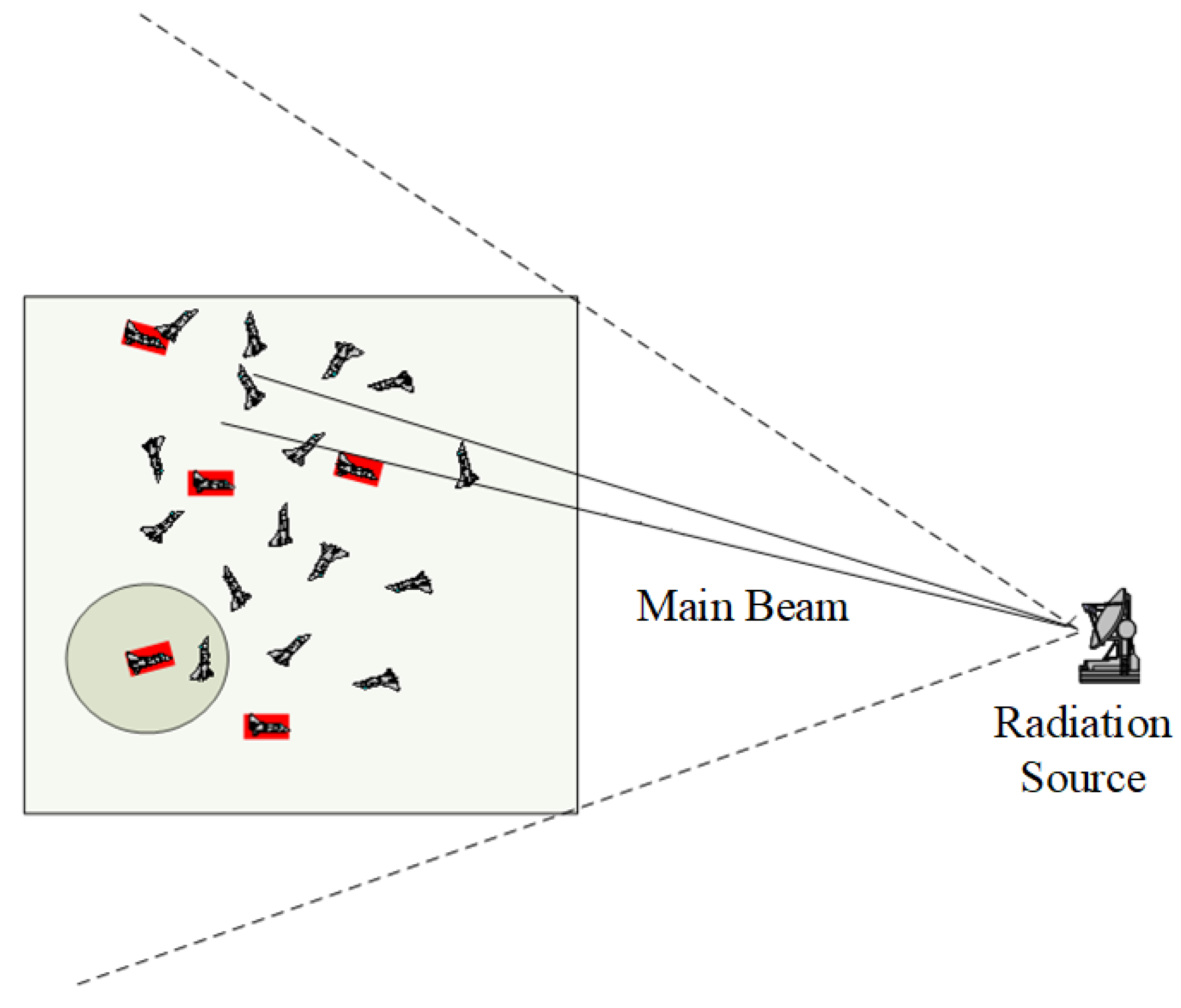
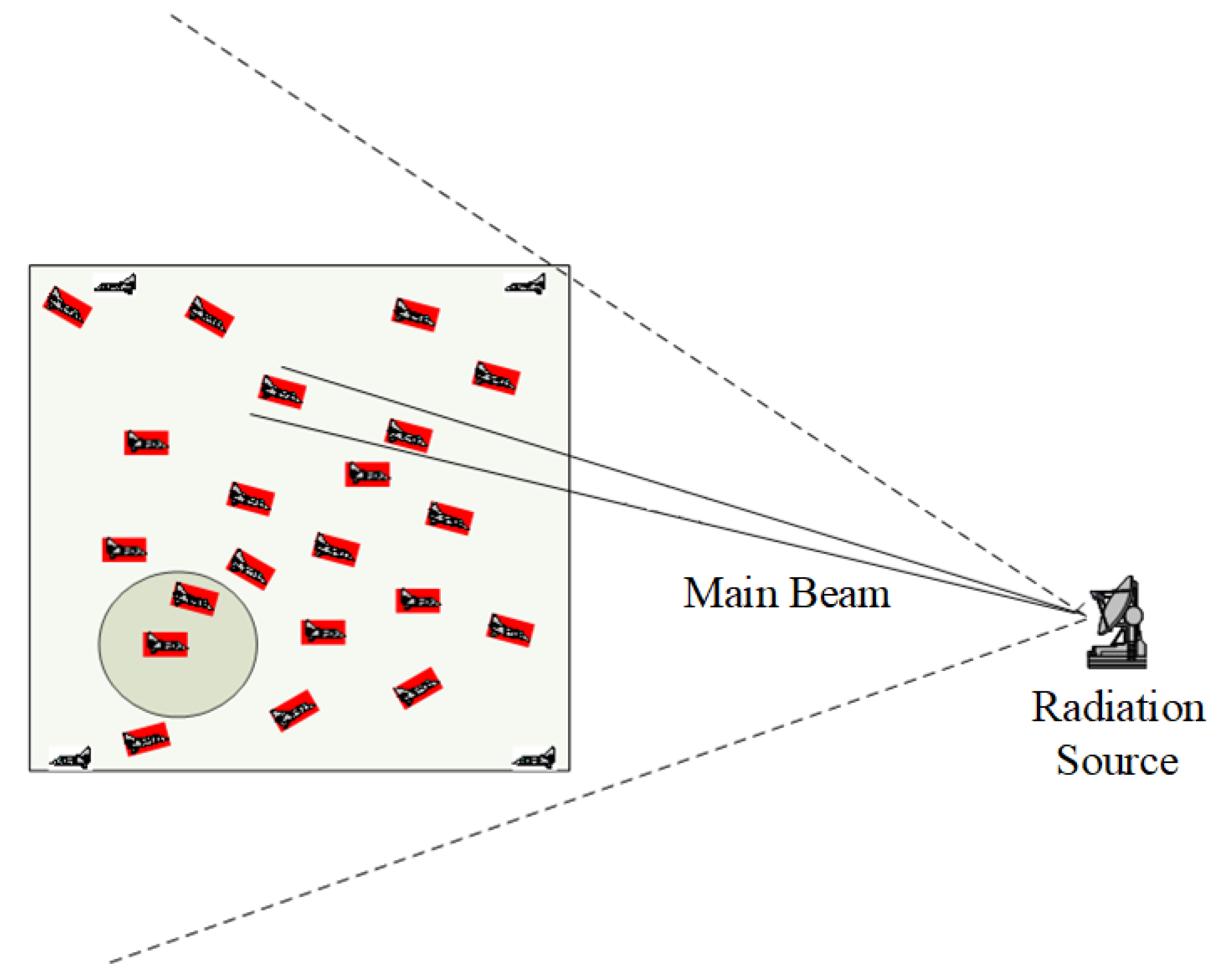
- (c)
- Radiation source information can be transmitted to the whole network through the pheromone transmission mechanism. Each UAV is weighted with other individuals within the communication radius to obtain the revised target location estimate .
4. Simulation Results
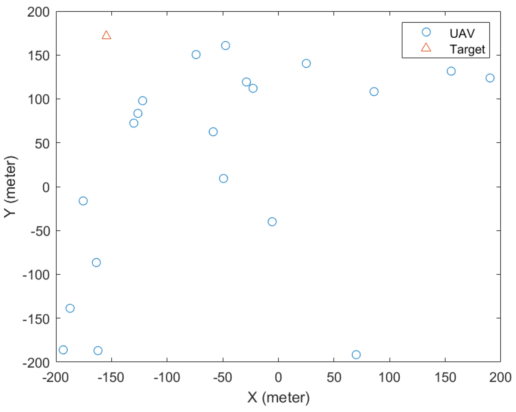
4.1. A Single-Fixed Target
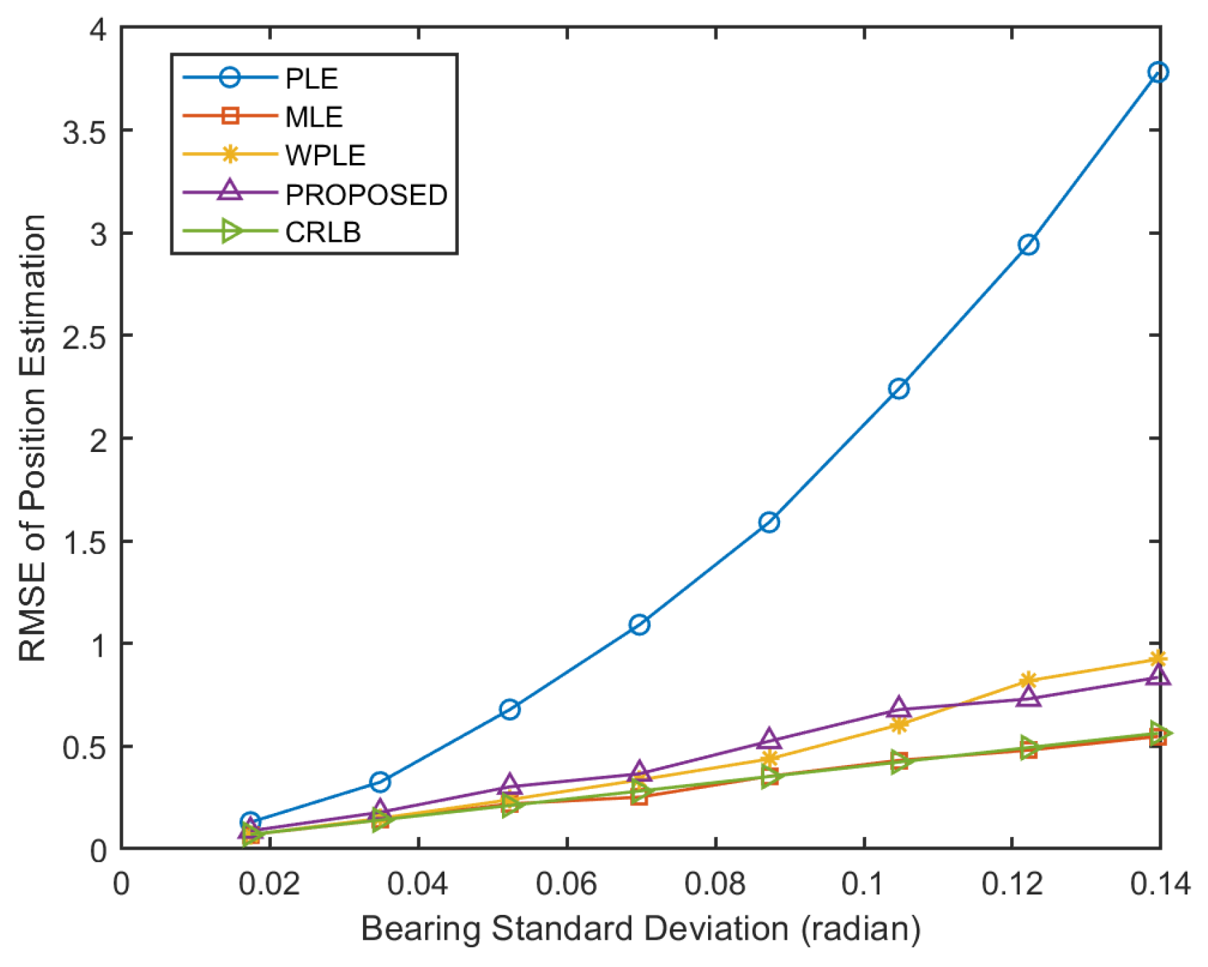
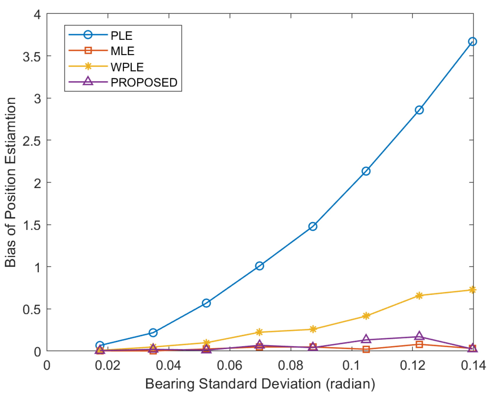
4.1.1. Bearing Standard Deviation
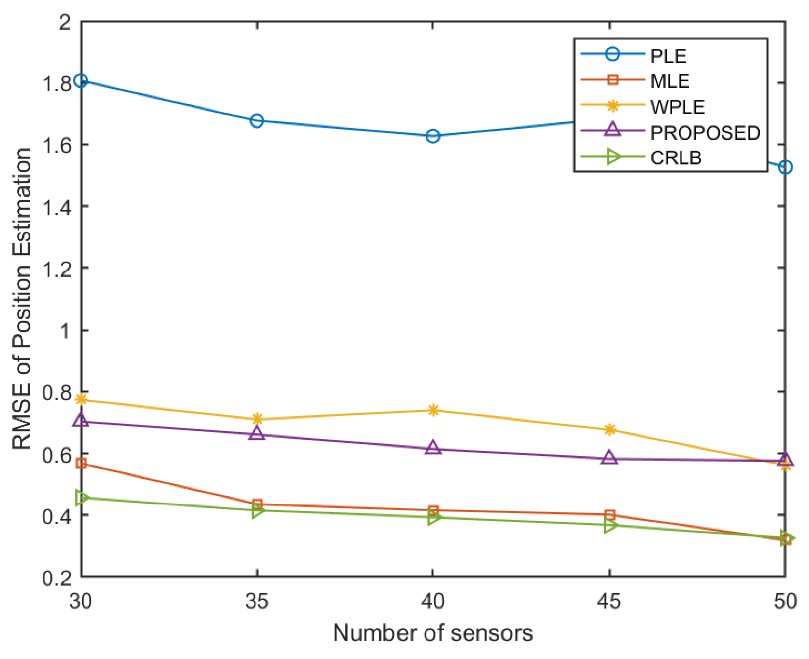
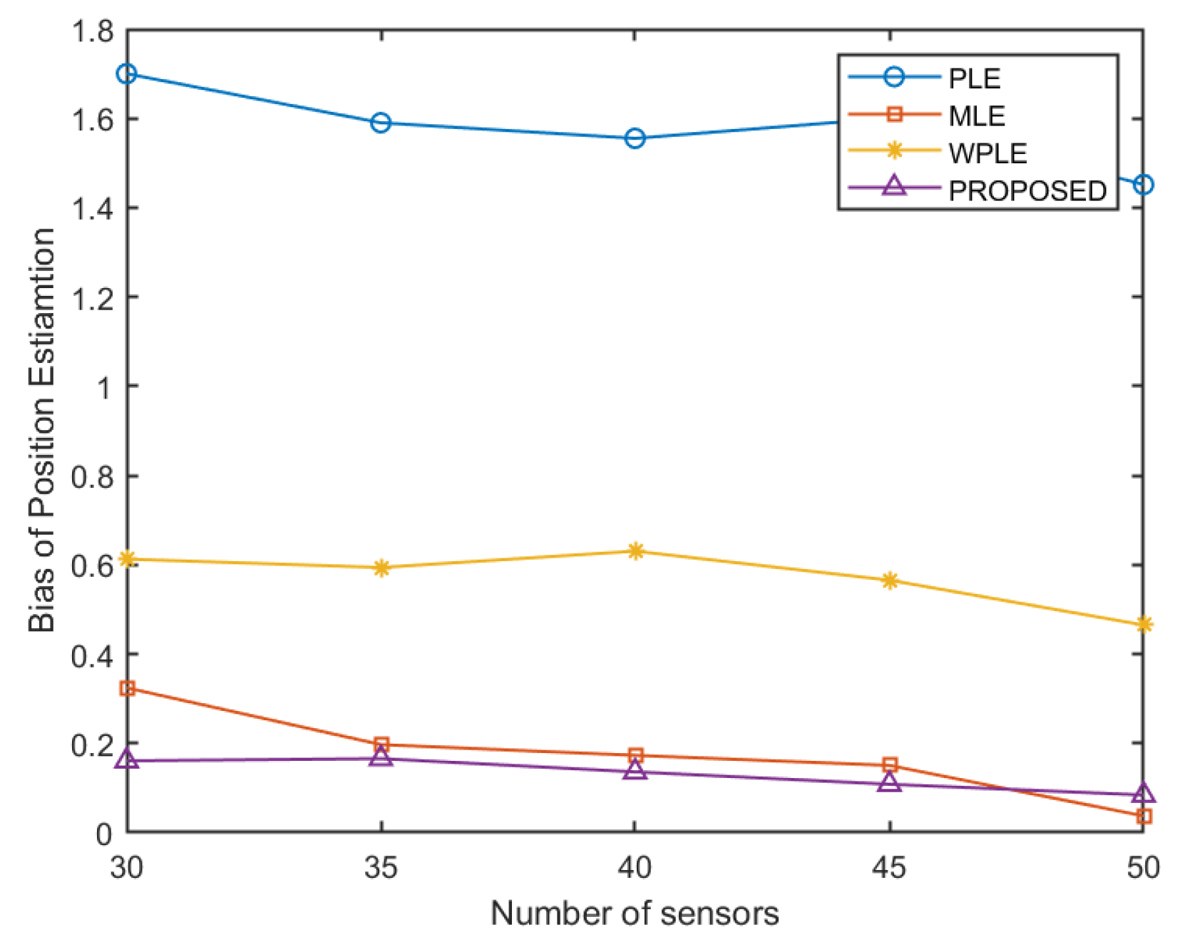
4.1.2. The Number of UAVs
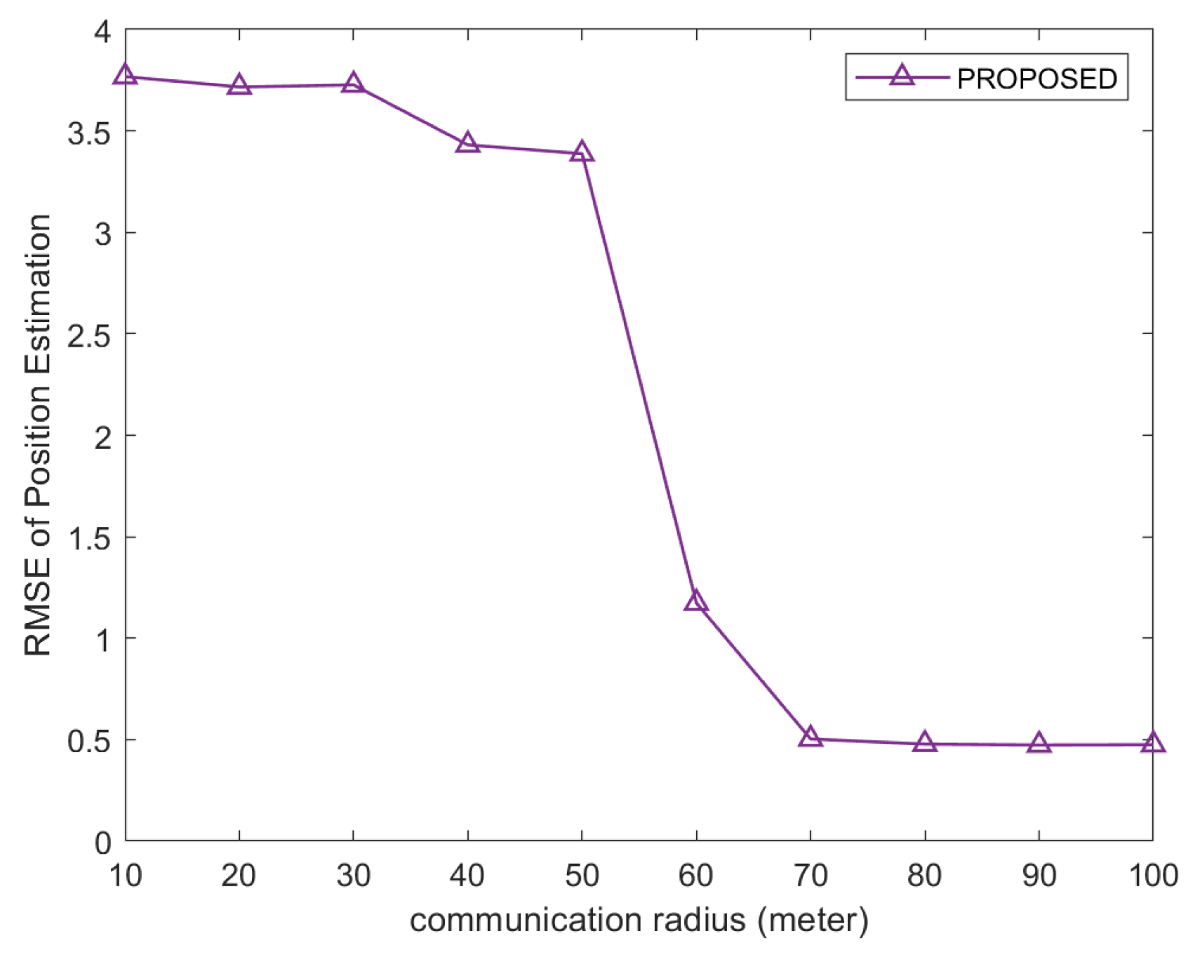
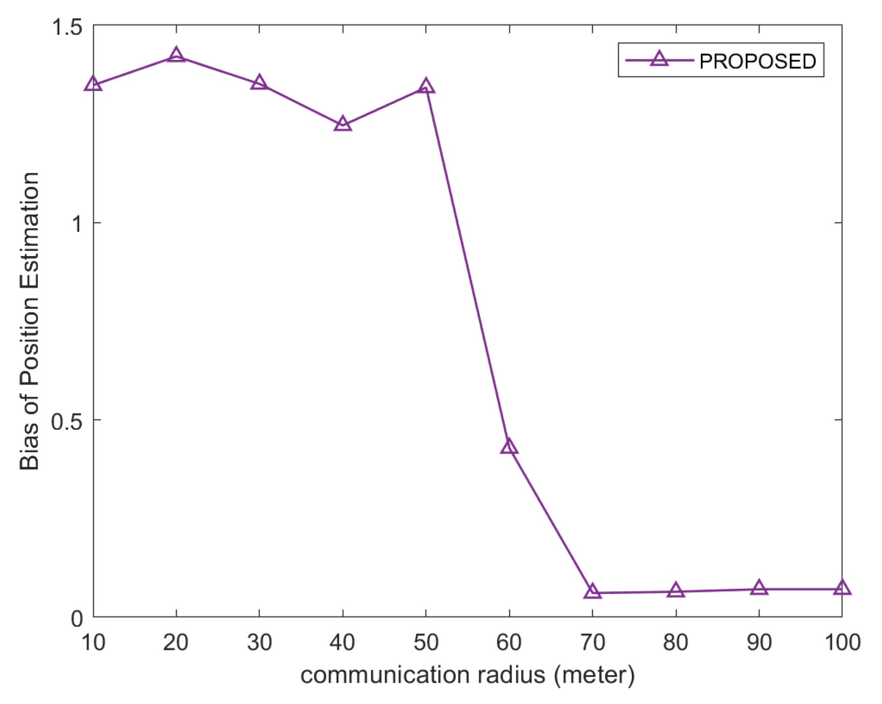
4.1.3. The Communication Radius of UAV
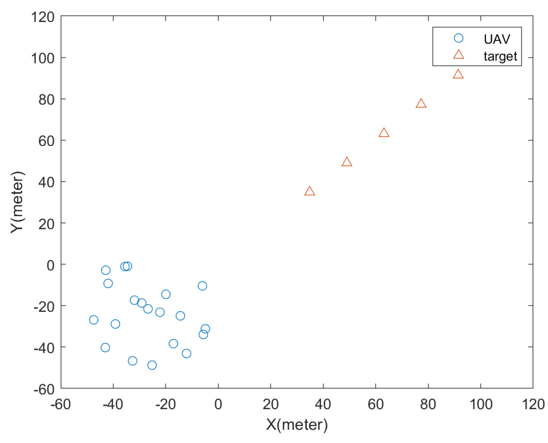
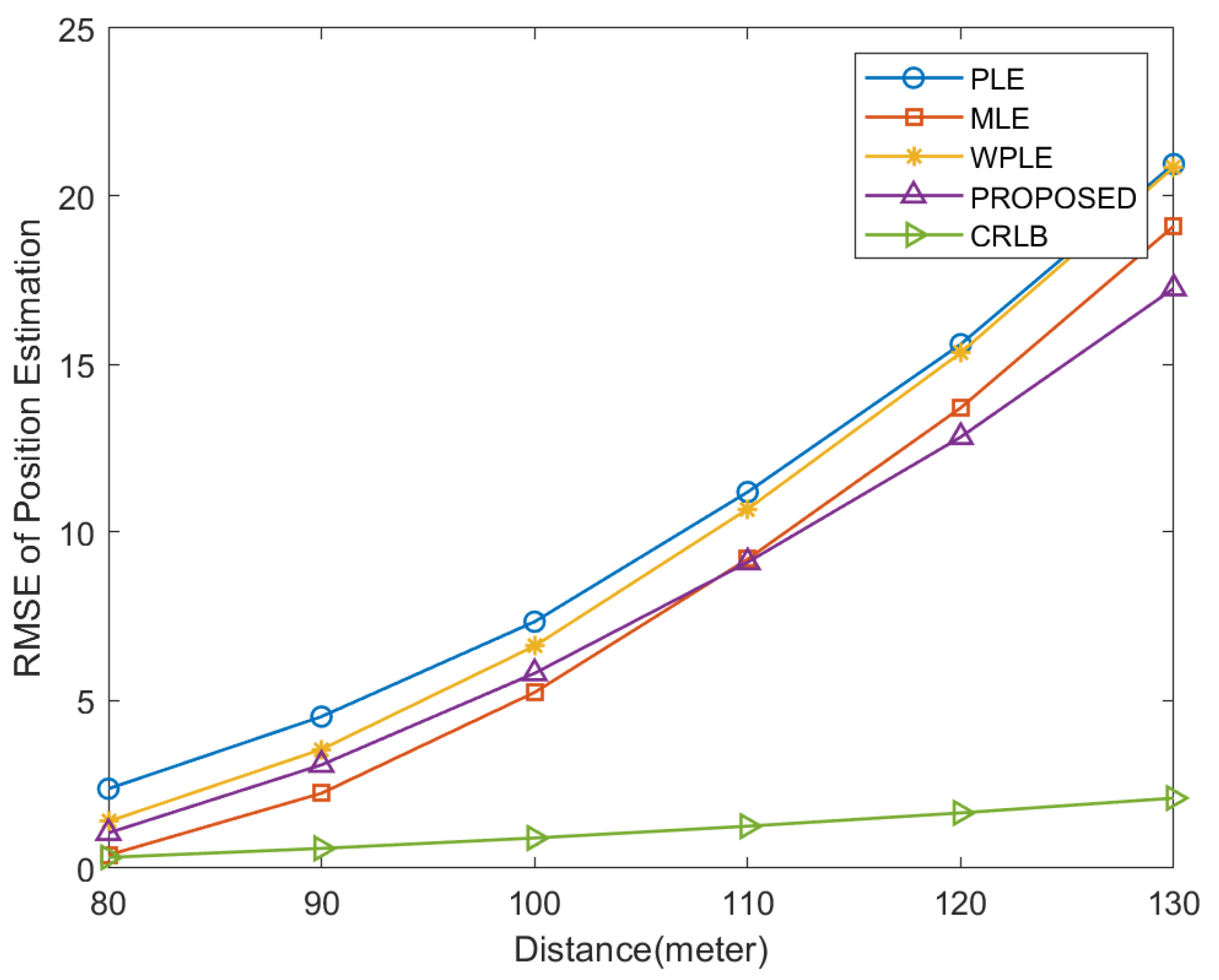
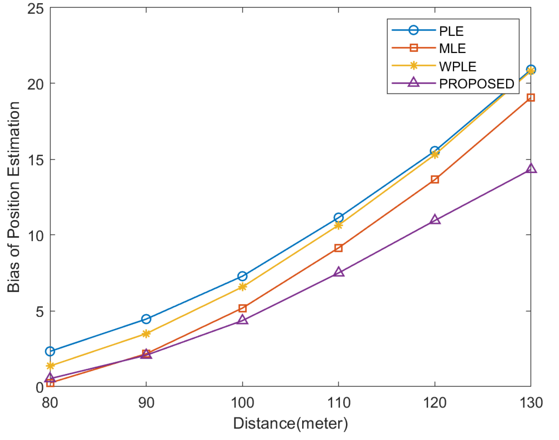
4.2. A Single-Unfixed Target
5. Conclusions
Author Contributions
Funding
Data Availability Statement
Conflicts of Interest
Abbreviations
| UAV | Unmanned aerial vehicle |
| PLE | Pseudo linear estimation |
| ML | Maximum likelihood |
| CRLB | Cramer-Rao lower bound |
| TDOA | Time difference of arrival |
| RSS | Received signal strength |
| FDOA | Frequency difference of arrival |
| AOA | Angle of arrival |
| LS | Least square |
| DWLS | Distance weighted least squares |
| NLOS | Non-line of sight |
| RMSE | Root mean square error |
References
- Zhou, Y.; Rao, B.; Wang, W. UAV Swarm Intelligence: Recent Advances and Future Trends. IEEE Access 2020, 8, 183856–183878. [Google Scholar] [CrossRef]
- Cheung, K.W.; So, H.C. A multidimensional scaling framework for mobile location using time-of-arrival measurements. IEEE Trans. Signal Process. 2005, 53, 460–470. [Google Scholar] [CrossRef] [Green Version]
- Yan, Y.; Wang, H.; Shen, X.; He, K.; Zhong, X. TDOA-based source collaborative localization via semidefinite relaxation in sensor networks. Int. J. Distrib. Sens. Netw. 2015, 11, 248970. [Google Scholar] [CrossRef] [Green Version]
- Nguyen, N.H.; Doğançay, K. Optimal geometry analysis for multistatic TOA localization. IEEE Trans. Signal Process. 2016, 64, 4180–4193. [Google Scholar] [CrossRef]
- Salari, S.; Chan, F.; Chan, Y.T.; Read, W. TDOA estimation with compressive sensing measurements and Hadamard matrix. IEEE Trans. Aerosp. Electron. Syst. 2018, 54, 3137–3142. [Google Scholar] [CrossRef]
- Xiong, W.; Schindelhauer, C.; So, H.C.; Liang, J.; Wang, Z. A neurodynamic optimization approach to TDOA-based IoT localization in NLOS environments. arXiv 2020, arXiv:2009.06281. [Google Scholar]
- Ouyang, R.W.; Wong, A.K.S.; Lea, C.T. Received signal strength based wireless localization via semidefinite programming: Noncooperative and cooperative schemes. IEEE Trans. Veh. Technol. 2010, 59, 1307–1318. [Google Scholar] [CrossRef]
- Coluccia, A.; Ricciato, F. On ML estimation for automatic RSS-based indoor localization. In Proceedings of the IEEE 5th International Symposium on Wireless Pervasive Computing 2010, Modena, Italy, 5–7 May 2010; IEEE: Piscataway, NJ, USA, 2010; pp. 495–502. [Google Scholar]
- Lin, L.; So, H.C.; Chan, Y.T. Accurate and simple source localization using differential received signal strength. Digit. Signal Process. 2013, 23, 736–743. [Google Scholar] [CrossRef] [Green Version]
- Hu, Y.; Leus, G. Robust differential received signal strength-based localization. IEEE Trans. Signal Process. 2017, 65, 3261–3276. [Google Scholar] [CrossRef] [Green Version]
- Ketabalian, H.; Biguesh, M.; Sheikhi, A. A closed-form solution for localization based on RSS. IEEE Trans. Aerosp. Electron. Syst. 2019, 56, 912–923. [Google Scholar] [CrossRef]
- Amar, A.; Leus, G.; Friedlander, B. Emitter localization given time delay and frequency shift measurements. IEEE Trans. Aerosp. Electron. Syst. 2012, 48, 1826–1837. [Google Scholar] [CrossRef]
- Lingren, A.G.; Gong, K.F. Position and velocity estimation via bearing observations. IEEE Trans. Aerosp. Electron. Syst. 1978, 4, 564–577. [Google Scholar] [CrossRef]
- Doğançay, K. Bearings-only target localization using total least squares. Signal Process. 2005, 85, 1695–1710. [Google Scholar] [CrossRef]
- Son, B.K.; An, D.J.; Lee, J.H. Performance analysis of AOA-Based localization using the LS approach: Explicit expression of mean-squared error. J. Sens. 2020, 11, 1–22. [Google Scholar] [CrossRef]
- Gavish, M.; Weiss, A.J. Performance analysis of bearing-only target location algorithms. IEEE Trans. Aerosp. Electron. Syst. 1992, 28, 817–828. [Google Scholar] [CrossRef]
- Wang, Z.; Luo, J.A.; Zhang, X.P. A novel location penalized maximum likelihood estimator for bearing-only target localization. IEEE Trans. Signal Process. 2012, 60, 6166–6181. [Google Scholar] [CrossRef]
- Rui, L.; Ho, K.C. Bias analysis of source localization using the maximum likelihood estimator. In Proceedings of the 2012 IEEE International Conference on Acoustics, Speech and Signal Processing (ICASSP), Kyoto, Japan, 25–30 March 2020; IEEE: Piscataway, NJ, USA, 2012; pp. 2605–2608. [Google Scholar]
- Xu, J.; Ma, M.; Law, C.L. AOA cooperative position localization. In Proceedings of the IEEE GLOBECOM 2008—2008 IEEE Global Telecommunications Conference, New Orleans, LA, USA, 30 November–4 December 2008; IEEE: Piscataway, NJ, USA, 2008; pp. 1–5. [Google Scholar]
- Wang, W.; Bai, P.; Zhou, Y.; Liang, X.; Wang, Y. Optimal configuration analysis of AOA localization and optimal heading angles generation method for UAV swarms. IEEE Access 2019, 7, 70117–70129. [Google Scholar] [CrossRef]
- Wan, P.; Huang, Q.; Lu, G.; Wang, J.; Yan, Q.; Chen, Y. Passive localization of signal source based on UAVs in complex environment. China Commun. 2020, 17, 107–116. [Google Scholar] [CrossRef]
- Wang, Y.; Ho, K.C. An asymptotically efficient estimator in closed-form for 3D AOA localization using a sensor network. IEEE Trans. Wirel. Commun. 2015, 14, 6524–6535. [Google Scholar] [CrossRef]
- Luo, J.A.; Zhang, X.P.; Wang, Z. A new passive source localization method using AOA-GROA-TDOA in wireless sensor array networks and its Cramér-Rao bound analysis. In Proceedings of the 2013 IEEE International Conference on Acoustics, Speech and Signal Processing, Vancouver, BC, Canada, 26–31 May 2013; IEEE: Piscataway, NJ, USA, 2013; pp. 4031–4035. [Google Scholar]
- Luo, J.A.; Tan, Z.W.; Peng, D.L. A novel bearing-assisted TDOA-GROA approach for passive source localization. Int. J. Intell. Comput. Cybern. 2018, 11, 2–19. [Google Scholar] [CrossRef]
- Werner, J.; Wang, J.; Hakkarainen, A.; Cabric, D.; Valkama, M. Performance and Cramer Rao bounds for DoA/RSS estimation and transmitter localization using sectorized antennas. IEEE Trans. Veh. Technol. 2015, 65, 3255–3270. [Google Scholar] [CrossRef]
- Tomic, S.; Beko, M.; Dinis, R. Distributed RSS-AoA based localization with unknown transmit powers. IEEE Wirel. Commun. Lett. 2015, 5, 392–395. [Google Scholar] [CrossRef] [Green Version]
- Ho, K.C.; Lu, X.; Kovavisaruch, L. Source localization using TDOA and FDOA measurements in the presence of receiver location errors: Analysis and solution. IEEE Trans. Signal Process. 2007, 55, 684–696. [Google Scholar] [CrossRef]
- Noroozi, A.; Oveis, A.H.; Hosseini, S.M.; Sebt, M.A. Improved algebraic solution for source localization from TDOA and FDOA measurements. IEEE Wirel. Commun. Lett. 2017, 7, 352–355. [Google Scholar] [CrossRef]
- Dexiu, H.U.; Huang, Z.; Zhang, S.; Jianhua, L.U. Joint TDOA, FDOA and differential doppler rate estimation: Method and its performance analysis. Chin. J. Aeronaut. 2018, 31, 137–147. [Google Scholar]
- Zhang, X.; Wang, F.; Li, H.; Himed, B. Maximum likelihood and IRLS based moving source localization with distributed sensors. IEEE Trans. Aerosp. Electron. Syst. 2020, 57, 448–461. [Google Scholar] [CrossRef]
- Aernouts, M.; BniLam, N.; Berkvens, R.; Weyn, M. TDAoA: A combination of TDoA and AoA localization with LoRa WAN. Internet Things 2020, 11, 100–236. [Google Scholar] [CrossRef]
- Vidal-Valladares, M.G.; Díaz, M.A. A Femto-Satellite Localization Method Based on TDOA and AOA Using Two CubeSats. Remote Sens. 2022, 14, 1101. [Google Scholar] [CrossRef]
- Luo, J.A.; Wang, Z. A novel closed-form estimator for 3D source localization using angle of arrivals and gain ratio of arrivals. In Proceedings of the 2017 36th Chinese Control Conference (CCC), Dalian, China, 26–28 July 2017; IEEE: Piscataway, NJ, USA, 2017; pp. 5179–5182. [Google Scholar]
- Baggio, A.; Langendoen, K. Monte Carlo localization for mobile wireless sensor networks. Ad Hoc Netw. 2008, 6, 718–733. [Google Scholar] [CrossRef]
- Pathirana, P.N.; Bulusu, N.; Savkin, A.V.; Jha, S. Node localization using mobile robots in delay-tolerant sensor networks. IEEE Trans. Mob. Comput. 2005, 4, 285–296. [Google Scholar] [CrossRef]
- Dong, L. Cooperative localization and tracking of mobile ad hoc networks. IEEE Trans. Signal Process. 2012, 60, 3907–3913. [Google Scholar] [CrossRef]
- Colorni, A.; Dorigo, M.; Maniezzo, V. Distributed optimization by ant colonies. In Proceedings of the First European Conference on Artificial Life, Paris, France, 11–13 December 1991; Volume 142, pp. 134–142. [Google Scholar]
- Guntsch, M.; Middendorf, M. Pheromone Modification Strategies for Ant Algorithms Applied to Dynamic TSP. In Proceedings of the Workshops on Applications of Evolutionary Computation, Como, Italy, 18–20 April 2001; Springer: Berlin/Heidelberg, Germany, 2001; pp. 213–222. [Google Scholar]
- Luo, J.A.; Shao, X.H.; Peng, D.L.; Zhang, X.P. A novel subspace approach for bearing-only target localization. IEEE Sens. J. 2019, 99, 8174–8182. [Google Scholar] [CrossRef]
- Wang, W.; Marelli, D.; Fu, M. Multiple-vehicle localization using maximum likelihood Kalman filtering and ultra-wideband signals. IEEE Sens. J. 2020, 21, 4949–4956. [Google Scholar] [CrossRef]
- Kay, S.M. Fundamentals of Statistical Signal Processing: Estimation Theory; Prentice-Hall, Inc.: Hoboken, NJ, USA, 1993. [Google Scholar]


Publisher’s Note: MDPI stays neutral with regard to jurisdictional claims in published maps and institutional affiliations. |
© 2022 by the authors. Licensee MDPI, Basel, Switzerland. This article is an open access article distributed under the terms and conditions of the Creative Commons Attribution (CC BY) license (https://creativecommons.org/licenses/by/4.0/).
Share and Cite
Zhou, Y.; Song, D.; Ding, B.; Rao, B.; Su, M.; Wang, W. Ant Colony Pheromone Mechanism-Based Passive Localization Using UAV Swarm. Remote Sens. 2022, 14, 2944. https://doi.org/10.3390/rs14122944
Zhou Y, Song D, Ding B, Rao B, Su M, Wang W. Ant Colony Pheromone Mechanism-Based Passive Localization Using UAV Swarm. Remote Sensing. 2022; 14(12):2944. https://doi.org/10.3390/rs14122944
Chicago/Turabian StyleZhou, Yongkun, Dan Song, Bowen Ding, Bin Rao, Man Su, and Wei Wang. 2022. "Ant Colony Pheromone Mechanism-Based Passive Localization Using UAV Swarm" Remote Sensing 14, no. 12: 2944. https://doi.org/10.3390/rs14122944