1. Introduction
In 2020, Poland’s construction sector attained peak efficiency (
Figure 1). It took twelve years to exceed the most severe Global Financial Crisis (GFC) of the century, which occurred in 2007–2008. This was the first year that residential construction in Poland reached levels that were last seen during the communist era. The difference from then to today is the high birth rate in the past, implying a large demand for additional housing as the postwar (WWII) baby-boomer generation entered the labor market, but there is currently population regression in Poland. Global urbanization trends, as well as international and domestic (country) migrations are all elements that support the development of cities and the urban functional areas that surround them. Specific conditions may be created by some characteristics that are dependent on geographic location.
At the end of 2019, the population in Poland was declining. The number of urban residents continued to decline, while the number of people living in rural areas increased [
1]. The greatest cities noted the influx of domestic (inter alia students) and foreign migrants (predominantly from Ukraine and Belarus) that were looking for employment and occupying apartments that were put up for rent by residents who had moved to the suburban and rural areas. The apartments in the city became a kind of investment that provided reasonable reimbursement for expenses incurred.
Suburbanization sprawl [
2], as well as inner-city trends, such as gentrification and reurbanization are at the forefront of urban growth. The pandemic outbreak of COVID-19 (which has been ongoing since 2020) and the start of the war in Ukraine (close to Poland) at the end of February 2022 have both caused chaos in recent years. Through the influence of so-called external factors, these “wildcards” will undoubtedly have major direct and indirect implications on individuals, particularly those living in metropolitan areas, as well as on cities themselves.
Figure 1.
Total dwellings completed per year in Poland 1950–2021; source of data: [
3].
Figure 1.
Total dwellings completed per year in Poland 1950–2021; source of data: [
3].
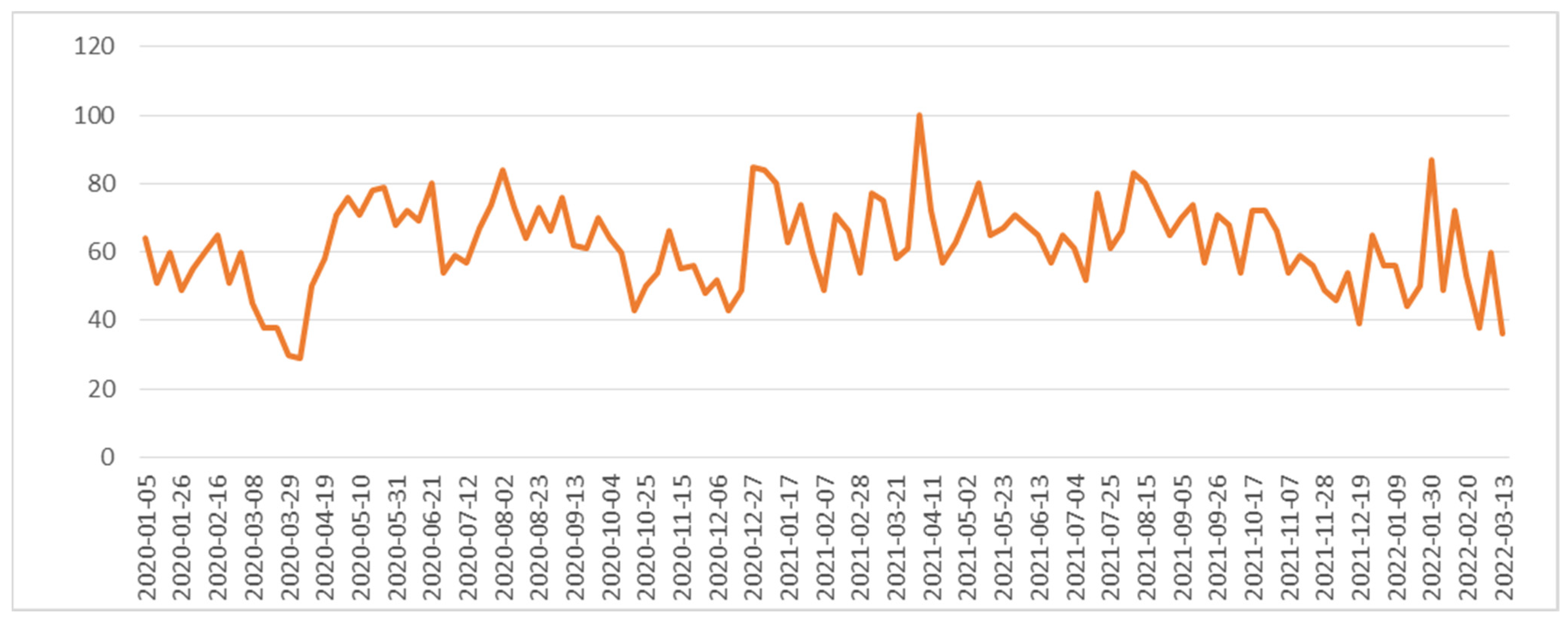
The main objective of the paper is to identify trends in the geographical development of urban areas in Poland over the last five years (2016–2021), particularly in terms of suburbanization sprawl processes, by looking for the driver factors that directly determine the spatial extent of observed processes, as well as other phenomena that may indirectly affect urban sprawl but are difficult to quantify and incorporate into a spatial analysis. During the COVID-19 lockdown periods (2020–2021), a much higher number of individuals tried to acquire residences that were outside of cities (
Figure 2), in order to migrate from city downtown areas.
According to statistics from the Polish Central Statistical Office, there were 1.39 million Ukrainian residents living in Poland by the end of February 2020, the final month before the epidemic outbreak. Later, some of them returned to Ukraine, but by the end of 2021 the University of Warsaw’s Centre of Migration Research projected that this group had grown to almost 1 million [
4]. However, the situation has now drastically changed. The unforeseen war in Ukraine on 24 February 2022 generated a massive (extra) flood of refugees from Ukraine, including women, children, and the elderly (
Figure 3).
Not all the refugees intend to remain in Poland. Some of them are moving further, but others, particularly males who previously worked in Poland, are returning to Ukraine to fight. For the time being the refugees are being relocated and housed; however, the Polish house-rental market has reacted quickly to their arrival. Contrary to the epidemic lockdown scenario a year ago which saw struggling market conditions, rental prices have now soared. Apartment rentals ceased to be successful businesses during the two-year COVID-19 pandemic (2020–2021). Students’ remote learning, tight borders for foreigners, working from home, and financial insecurity have all pushed tenants to flee the once-booming market.
These reasons, among others, appear to be crucial for the current development of urbanization in Poland. However, it would be worthwhile to investigate Poland’s suburbanization expansion over the previous five years, in order to see if worldwide patterns are still present in Poland before and during the epidemic, as well as now in a very different international and national situation.
However, the main hypothesis of this study is that inexorable worldwide trends in suburbanization sprawl [
7] will have remained stable and persistent in Poland since 2016, despite consideration of the diverse influence of stimulant, destimulant, and nominant variables that are assumed to affect the observed phenomenon. However, these processes may occur at different times, according to location [
7].
Finally, disruptive consequences that are significant for the housing market and rooted in both COVID-19 and the war in Ukraine include observed inflation and the continuous growth of all prices around the world in 2022, as well in Poland, which will probably also affect urbanization development.
2. Factors of Urban Sprawl
Suburbanization is defined as the movement of people to the suburbs, resulting in the fast expansion of city outskirts and urban sprawl. While the terms are sometimes interchanged, urban sprawl is typically linked with the unplanned and unregulated nature of suburbanization, as well as its multiple negative consequences, such as poor accessibility, a lack of usable open space, and high environmental costs. “A variety of definitions for sprawl have been put forth that describe sprawl as a specific form of urban development with low-density, dispersed, auto-dependent and environmentally and socially-impacting characteristics” [
8].
In an attempt to capture urban sprawl, a variety of basic and synthetic indicators were developed throughout the previous decade [
9,
10,
11]. Despite heated debates, virtually all of these multiple indicators are based on land uptake and population characteristics, with a strong inclination to examine population density inside built-up regions rather than over a unit’s whole territory [
2].
Although urban sprawl refers to the urbanization of suburbs, quantifying it requires a comparison of the relevant indicators for both urban areas (which are losing their functions) and urbanizing peripheral areas (which are gaining new inhabitants) over time, i.e., at least at the beginning and end of the analyzed period.
Individual decisions on where to live and work for a better quality of life fuel urban sprawl. Numerous socioeconomic and demographic factors, including land and apartment prices, transit availability, the desire for better living standards, and inner-city difficulties might hasten this process (
Figure 4).
According to recent data, urbanization in general and urban sprawl, in particular, became progressively detached from demographic dynamics (such as population increase) between 1990 and 2014. This is most likely the outcome of household migration from city centers to peripheries [
13]. Some extensive forecasting models take the ethnic makeup of the population into account as a component of suburbanization [
14]. Increases in the percentage of ethnic minority populations inside cities have been linked to an increase in urban sprawl in the United States [
15]. In a European environment, ethnic minority groups had the reverse effect [
16].
The majority of extant definitions for urban sprawl contain three spatial aspects: the growth of the urban area, the increase in build-up area dispersion, and low-density development in suburbia with a large land-take per person [
17,
18].
Residential suburbanization is not always associated with a permanent dwelling. While certain cities have seen seasonal population transfers to “second houses” [
19], the possible wildcards of suburbanization remain unexplored [
20].
3. Wildcards (Black Swans)
The “wildcards” or “Black Swans”, as described by Taleb [
21] are unanticipated (astonishing, shocking) events that are commonly regarded as rare, but whose occurrence might have a significant impact on people’s lives (societies). Wildcards are defined by a triplet of characteristics: uncommon outlier, severe impact, and retroactive (but not prospective) prediction of the event [
21].
Two such wild cards have occurred in recent years that overlap in time. The global COVID-19 outbreak in early 2020 and the war in Ukraine since February 2022. Both of these events have already had a huge impact on different parts of European society and the EU economy, especially in countries neighboring Ukraine (including Poland).
Looking back on the previous two years of COVID-19 in Poland [
22,
23], it is difficult to determine if the global pandemic is nearing its end. On the other hand, no one can predict if the conflict in Ukraine will extend longer (similar to Russia’s invasion of Crimea, Donetsk, and Lugansk in Ukraine in 2014) or whether a peaceful solution will be found shortly.
Surely, the external effects of these two “wildcards” will have a big impact on Polish society and the economy.
4. External Effects
Externalities are present in all human actions, including, of course, economic activities. They are often characterized as the unintended consequences of production or consuming activity that impact persons who are not directly involved in that activity. People are affected by externalities regardless of their volition, and their influence might be positive or negative. Externalities are either additional benefits or societal costs that are not factored into the economic activity calculation. Externalities are thought to be caused by the link between the economy and the environment.
Environmental pollution, landfill location, vandalism, social pathologies, and crime are examples of negative externalities. Positive economic spillovers are linked to service economies of scale, the advantages of agglomeration—location and urbanization, and, more recently, the advantages of globalization. They are viewed as unanticipated profits from spillover effects in economics [
24].
“Broadly defined, spillovers, or other economic neighborhood effects, refer to unanticipated changes in the well-being of the population, i.e., the actions of individuals or third parties, and sometimes events that indirectly affect other people’s standard of living. The costs or rewards of externality effects are not included in the direct account of economic activity” [
25]. Spillover effects were characterized by Marshall [
26] as market externalities of economic activity, whereas Pigou [
27] defined them as variations in societal and private costs and benefits. Mishan [
28] provided a more detailed and slightly different definition of externalities, which he defined as the expected (anticipated) or unanticipated spillover effects of third-party activities that directly or indirectly affect changes in people’s living standards.
Growth pole theory interprets externalities as differences in the action of centripetal and centrifugal forces, concentration and dispersion, or attraction and repulsion [
29], explaining the spatial order and patterns of urbanization [
30,
31,
32]. Externalities are divided into financial and technological impacts, sectoral and urbanization effects, positive and negative effects, and productivity (labor) or development (regional) effects. Regardless of categorization, a case-by-case analysis is the most common method for describing externalities in-depth [
33].
5. Spatial Externalities
The examination of spatial externalities is one component of land-use change research, which involves tracing suburban sprawl [
34]. Spatial externalities, on the other hand, are the unintended, indirect consequences of human actions that result in a drop in value (extra cost) or a rise in value (additional gain) for others [
28]. The intensity (rate) and spatial extent of land-use change externalities are frequently revealed. There is a difference between negative and positive spatial impacts. It is thought that the higher the degree of externalities in a specific land-use class (for example, built-up regions), the greater the likelihood of land-use change in that place [
35].
6. Materials and Methods
6.1. Location Quotients
Due to the requirement to attain relatively recent geographical and statistical data, the index that was used as an independent variable, measuring suburbanization sprawl up to 2021, was new Dwellings Completed per 10,000 inhabitants (per 10K) within counties and communes (and municipalities), and functional urban areas (FUA) in Poland from 2016 to 2020 (in every year). The index assumed that the spatial extent of frontline urban expansion, particularly suburbanization sprawl, was determined by the geographical location and volume of new investments in certain years. Official data were acquired from Statistics Poland (CSO) (The CSO database status was updated to 2020 for communes as of 20 May 2022) [
2].
Dwellings Completed per 10K-absolute values and location quotients (LQ) by counties, communes, and functional urban areas were observed. The index of Dwellings Completed per 10K for the relevant county for a certain year was the reference figure for estimating a particular LQ in a commune within the spatial extent of a certain county.
Location quotient (LQ
i), or regional index, for a spatial unit (region) is the ratio of the value of an indicator of a specific economic or social activity
Si in spatial unit
i (commune
i) to the value of that indicator A in a higher spatial unit (county, Equation (1)) [
36]:
where:
Si—Dwellings Completed per 10K in certain commune (municipality) annually,
A—Dwellings Completed per 10K in relevant county annually (and in relevant FUA). This way, each commune obtained five LQ indices, separately for each observed year.
LQ also creates the possibility of comparisons for different points in time, thus fulfilling a function similar to the standardization of features. LQ < 1 indicates a ‘shortage’ of residential construction in the county, compared to the national value. LQ > 1 reveal ‘overrepresentation’, i.e., the spatial concentration of residential construction [
36]. Assuming the frontline of suburbanization sprawl shows the relatively high persistent LQ of dwellings that were completed over an observed time, the harmonic mean of the above LQs for each commune was calculated. The choice of harmonic means was dictated due to operating the relative values for a space–time series. Classification of the harmonic means commune data are presented as follows in
Table 1.
6.2. The Global Human Settlement Model (GHS-SMOD)
The GHS Settlement Model layers (GHS-SMOD) delineate and classify settlement typologies via a logic of cell clusters’ population size, population, and built-up area densities as a refinement of the degree of urbanization. The second hierarchical level of the GHSL SMOD (L2) classification is a refinement that aims to identify smaller settlements. The input data are the multi-temporal GHS-BUILT and GHS-POP grids of the GHSL Data Package 2019 (GHS P2019). The land is extracted as a combination of the Global Administrative Map 2.816 and the Global Surface Water Layer Occurrence. Names are extracted from OpenStreetMap partially filtered by EUROSTAT (GISCO project) [
37].
The set of LQ harmonic means of communes in Poland was next spatially and statistically compared to the Global Human Settlement Layer data that were clipped for Poland. The used data were part of GHS Settlement Model Layers (GHS-SMOD), derived from GHS-POP (population) and GHS-Built (built-up). The data present the classification of grid spatial entities as follows in
Table 2.
Next both data sets were statistically and spatially analyzed using the available Zonal Histogram and cross-tabulation tools of GIS software. Statistical analyses of LQ by communes (municipalities) do not provide information on the exact localization of urban sprawl. This is why the spatial analysis used the reclassified results of a comparison of two nominal-scale input-raster layers: LQs by communes and GHSL layer (vector layers of communes were rasterized to the same grid system as GHSL). Processing the overlay of the input layers was based on the concatenation of nominal values: two-digit number of GHSL and one-digit number of LQ class (e.g., Urban Centre descriptor 30 and class 2 of harmonic mean LQ give a result equal to 302). In fact, this is a simple raster calculator expression: [GHSL class integer number × 10 + LQ class integer number]. Eventually, the results were presented cartographically using a bivariate color legend.
Another thread of the study concerning the comparison of estimated LQ used, as the reference, the relevant-for-commune values of Dwelling Completed per 10K that were calculated for particular functional urban areas (FUA) in Poland where the commune was located. For the communes outside FUA borders, the reference value was the average indicator. A cartographical presentation of the results aimed to highlight the differences.
The operationalization of the study used the software packages GIS (ESRI ArcGIS, QGIS) and statistical (SPSS). The technical details of cross-tabulation, clipping, and the spatial transformation of resulting maps also concerned their re-projections, as well as rasterization and generating the common attribute tables of joined maps.
7. Results
7.1. Urban Sprawl in Poland in Light of Dwellings Completed per 10K Population
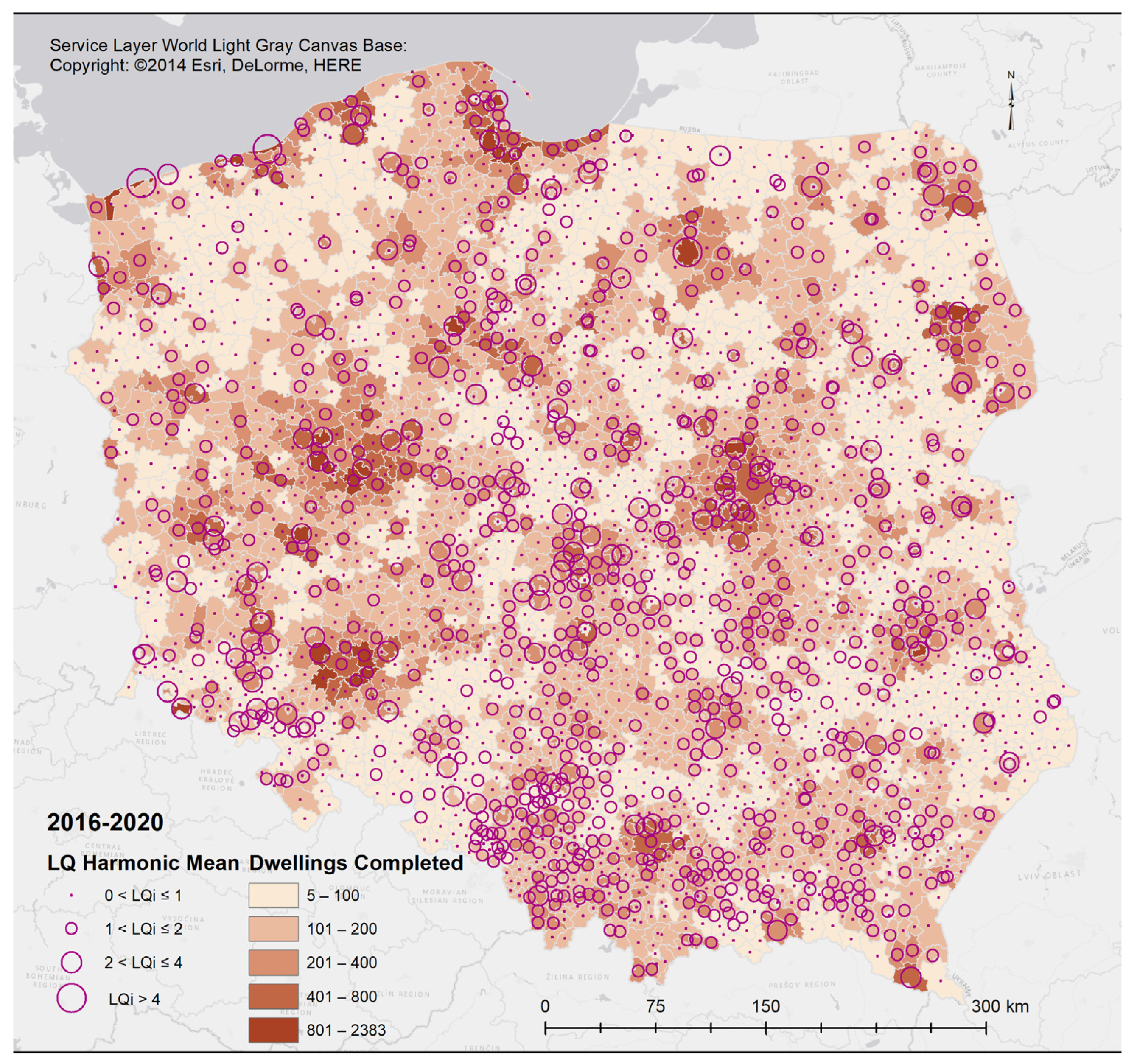
Since 2016, the building sector in Poland has seen a steady increase in the number of houses constructed per 10K. The number of houses built per 10,000 people varied based on the size of the commune and its location. The total number of dwellings that were completed and the harmonic mean of location quotients by communes in Poland from 2016 to 2020 are presented in
Figure 5. The spatial diversity of the absolute values of the total dwellings completed per 10K population by communes reveals specific ‘bagels’—areas surrounding the greatest metropolises that also surpass urban centers. The spatial diversification of the harmonic means of LQs is similar, but not identical to the spatial pattern of total absolute values.
Despite minimal variations over the observed time, the general trend was the continuous growth of dwellings completed per 10K from 2016 in a large number of communes (
Figure 6). Only minor details of the spatial diversity of the examined phenomena were observed throughout the years preceding the COVID-19 pandemic epidemic (2016–2019).
It seems that the first year of the COVID-19 pandemic outbreak in Poland (2020) did not change much in the residential construction sector.
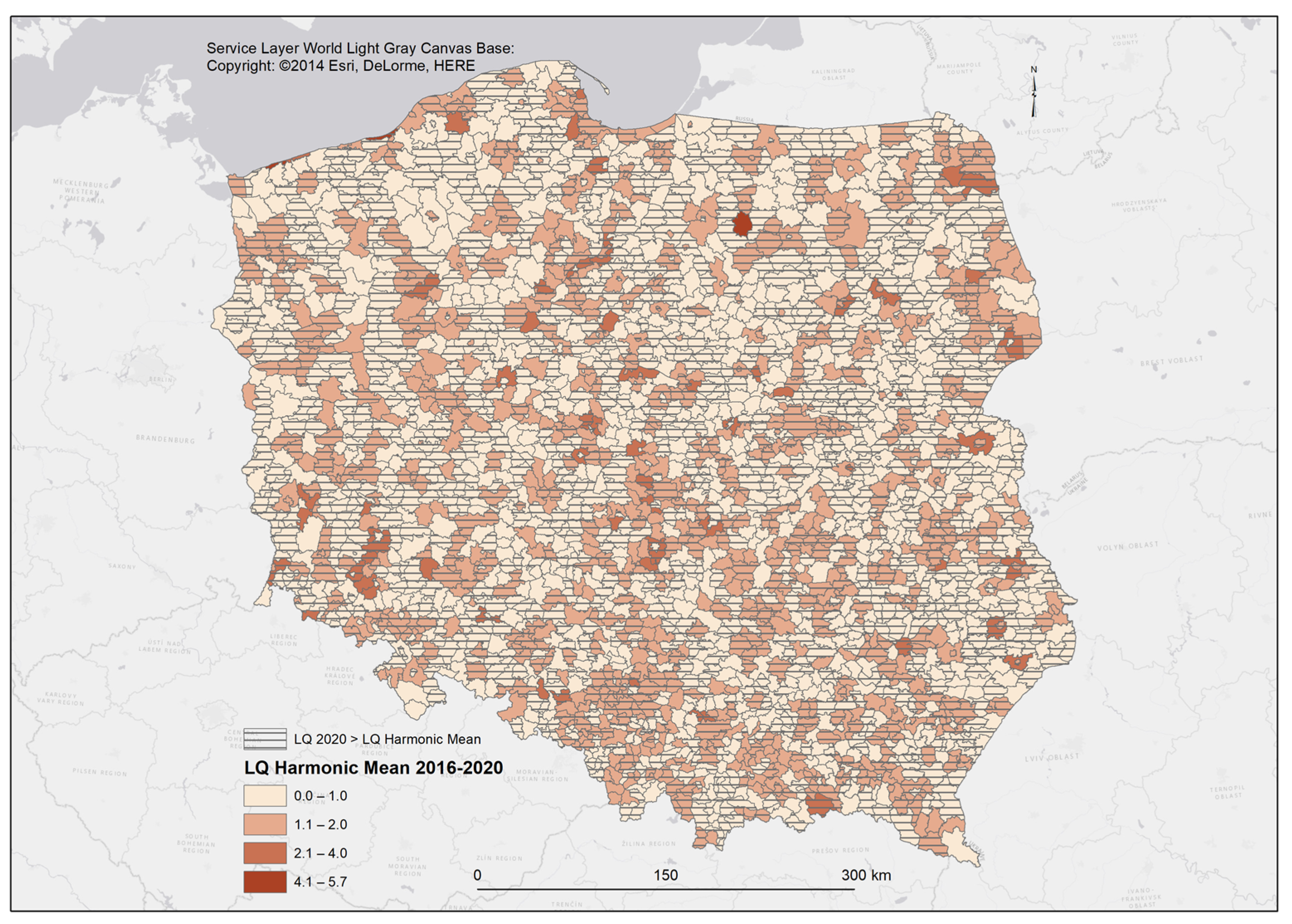
Figure 7 presents the spatial distribution of the location quotient-harmonic means of dwellings that were completed. Communes marked with the lines fill symbol for those LQ in 2020 are greater than the harmonic mean LQ for the whole observed time.
The situation of urban sprawl in Poland in 2021 changed. It should be noted that from August to December, tensions over the ‘push and pull’ of illegal immigrants occurred in the region of North-East Poland near the Belarus state boundary. Visitors were not permitted to enter the special zone along the EU-Belarus-Poland border. The zone along the Poland-Belarus border experienced (locally) the temporary delays in private investments, except for when the state ordered the construction of the temporary border fence in 2021 (a solid fence that continues to be built in 2022). The overall length of the solid fence will be 180 km, 5 m high, and equipped with CCTV monitoring and movement-detection sensors. The only great city in the Podlaskie region, tenth in terms of populated places in Poland is located 60 km from the Belarus border (not in a closed zone).
In turn, from 24 February 2022, external conditions changed drastically. Poland has been the target of the massive influx of Ukrainian refugees fleeing the war. It is probable that the first wave mostly comprised the families of Ukrainian citizens who earlier worked in Poland and thus have a place to shelter themselves. After a few weeks, others fled from Eastern Ukraine. It is unknown how many people will yet flee from Ukraine, targeting or transiting Poland.
The two external forces mentioned above will produce opposing processes. The continuation of global COVID-19 pandemic waves (for example, new SARS-COV2 virus variants in future autumn and winter seasons) poses a new threat to Poland’s economic development, whereas the massive influx of Ukrainians could be a stimulus, especially if they decide to stay in Poland for a longer period. Time will tell how these disastrous events will affect Poland’s residential building sector and rental housing market. There is currently no official published data available on the quantity and location of new residential units and dwellings completed.
7.2. Statistical and Spatial Analysis of Urban Sprawl in Poland Using GHSL Layer
A statistical analysis was carried out using the Zonal Histogram tool and tabulating areas for a defined subset of the GHS-SMOD layer for Poland using GIS software. The intermediate result was the attribute table of the communes’ layer in Poland, involving columns from both input sets: the values of the harmonic means of location quotients, and the cell count (areas) of each distinguished class in the GHS-SMOD layer within the extent of the relevant commune. Due to the nominal scale of both reviewed phenomena, a nonparametric Spearman’s rho association was estimated between the variables. The results are presented in
Table 3.
There were 29 significant (2-tailed) correlation coefficients from 48. A large number of them were very close to zero. However, only one GHS-SMOD layer class—suburban or peri-urban areas or semi-dense areas were relatively higher, and positively correlated to the harmonic mean location quotient (R = 0.402). Similarly, all of the location quotients for the above class were significant and higher than for the other classes within the range [+0.303, +0.344].
A repeated statistical analysis of the correlation between the LQ harmonic means and suburban and peri-urban class using Kendall’s Taub coefficient gave a similar significance but a lower value (R = 0.3). These values are not high but taking into account the range of other Spearman’s rho coefficients [−0.142, +0.155] for other GHS-SMOD classes, it means that a moderate association between LQ harmonic means and sub- and peri-urban areas seems significant.
Spatial analysis geovisualization used a bivariate colors legend for a choropleth map for all the above-enumerated variables. The legend uses the four colors analog that is proposed in the GHS-SMOD layer. The LQ harmonic means values are divided into the classes described above (
Section 6). The intense depth of colors shows low levels of harmonic means of location quotients, contrary to pale colors which relate to high values of LQ harmonic means (2016–2020), which is a metaphor for the anthropogenic pressure that is related to the volume of artificial light emission. Green colors are related to the very low- density rural class (GHSL code 11) and near water (GHSL code 10) within the particular commune. Yellow to orange colors represent the low density rural and rural areas (GHSL codes 12 and 13). Semi-dense urban and sub-urban or peri-urban areas (GHSL codes 21 and 22) are represented by pink colors, and the violet color scales are related to urban centers and dense urban areas. Light shades of colors reveal areas that are the border zones of urban sprawl.
All location quotients by communes are calculated using an annual number of dwellings completed per 10K population to the referenced values for higher administrative units, i.e., annual dwellings completed within the appropriate counties (
Figure 8).
Another study thread involved comparing the estimated LQ, using as a reference the relevant commune values of Dwelling Completed per 10K that were summed up for certain functional urban areas (FUA) in Poland where the commune was located. The average indication was used as the reference value for communes that were outside of the FUAs. The data were presented in a cartographical format to emphasize the differences (
Figure 9).
8. Discussion
In an analysis of the spatial diversity of location quotients’ harmonic means covering the period from 2016 to 2020 (
Figure 5), one must note the evident process of urban sprawl. When interpreting the high values of the harmonic means of LQs as the rate of urban sprawl, almost all communes characterizing the pace of the new dwellings completed are located nearby, outside the main metropolises of Poland and around dense towns, as well as close to the main touristic destinations offshore of the Baltic Sea (in the North), and in mountains (in the South). On the other hand, the centers of urban areas (e.g., Warsaw, Gdansk, Wroclaw, Poznan, and Lodz) and dense smaller cities (Olsztyn, Koszalin, Rzeszow) usually characterize a slightly lower pace and number of dwellings completed. A higher pace of location quotients is also observed near land border crossings. It seems that the first year of the COVID-19 pandemic outbreak in Poland (2020) did not change much in the residential construction sector, and the inertia of previous years’ trends was sustained. This could be a time lag related to the lifecycle of the construction process (from the approval of an investment plan to construction completion). Isolation and lockdown restrictions related to the two-year pandemic situation caused most people living in cities (especially in multi-family houses) to start to look at plots outside of the cities, which had an impact on the prices of the real estate market. However, no officially published recent data are available on dwellings that were completed in 2021. Nevertheless, all the above-mentioned external factors, the pandemic, and the crisis along the Poland–Belarus border (in the North-East, related to an influx of illegal immigrants), as well as growing inflation, resulted in the rising prices of building materials and apartment rentals. These tendencies are reinforced because of the outbreak of the war in Ukraine (the South-East border line of Poland), which again intensified the pace of inflation in 2022. All these critical events may indirectly and strongly affect the urban sprawl in Poland in the forthcoming years.
Significant confirmation of the observed urban sprawl processes in Poland gave a statistical analysis of the Spearman’s rho correlation coefficients between the harmonic means LQ and GHSL classes of main urban and rural regions. This was not in terms of the strength of the association, but by excluding all of the types except only one: suburban and peri-urban areas, which is the direct validation of the observed relation.
Statistical LQ analyses by communes (municipalities) do not give precise information on the precise extent of urban sprawl. As a consequence, the findings of the comparison of two nominal-scale input-raster layers were used: LQs by communes and the GHSL layer, which were reclassified and aimed at a spatial analysis; two approaches were taken into account.
First, a comparison of the harmonic means of LQs of communes referred to counties and a subset of the GHSL layer that was clipped to the borders of Poland. The resulting map (
Figure 8) reveals irregular zones of urban sprawl around the metropolises and dense towns along the main exit routes, which characterize class semi-dense urban cluster spatial entities and suburban or peri-urban with the highest LQs. It also shows insular, separated areas within the rural cluster-spatial entities zones with higher LQs nearby the small towns in the centers (probably the second houses zones or touristic destinations).
Second, a comparison of the harmonic means of LQs of communes referred to functional urban area zones in Poland and a subset of the GHSL layer that was clipped to the borders of Poland. The resulting map (
Figure 9) is more distinct and the zones of urban sprawl are clearer. The shape of zones is more regular.
9. Conclusions
Despite Poland’s strong residential building development trend, it is difficult to predict if urban expansion, particularly suburbanization sprawl, will continue to a larger spatial extent due to insufficient critical spatial-infrastructure investments outside of city limits. Our research is very broad and based on recently acquired and only recently available data, and it appears that there is a need for a deeper understanding of the processes of change in the spatial, social, and economic structure of functional urban areas, which would require unavailable recent data; for example, detailed data of the functional urban areas in Poland (as well as other EU countries) and Global Human Settlement Layer data that only cover the year 2018. Further, the findings of the recently concluded national population census (2021) will be released in full in the near future.
Synergetic (potentiating) effects and feedback that are distinct to various geographic locations are shaped by the action of several elements. For example, urbanization in Ukraine was estimated at 69.6% by the end of 2021, while it was only 60% in Poland by the end of 2020 [
39]. People from Ukrainian cities make up the majority of Ukrainian refugees. Their environment was urban, and they arrived in Poland’s major cities searching for (at least) temporary lodging, or lodging that was comparable to the kind found in Ukraine. This implies that Poland’s cities would be under huge pressure.
The cumulative impact of factors influencing the spatial development of cities is not the simple sum of them, rather, they act in a compounded way. However, the synergy of the influence of a different number of factors in different geographical areas may not be the same. Thus, one can expect different processes and spatial extents of the urban sprawl of Polish cities.
Author Contributions
Conceptualization, P.A.W.; methodology, P.A.W.; software, P.A.W. and M.P.; validation, P.A.W.; formal analysis, P.A.W.; investigation, P.A.W. and V.K.; data curation, P.A.W. and M.P.; writing—original draft preparation, P.A.W. and V.K.; writing—review and editing, P.A.W., V.K. and M.P.; visualization, P.A.W. and M.P.; supervision, P.A.W.; project administration, P.A.W.; funding acquisition, P.A.W. All authors have read and agreed to the published version of the manuscript.
Funding
This study was financed by the IDUB project granted by University of Warsaw under the program Excellence Initiative: Research University (IDUB).
Data Availability Statement
Conflicts of Interest
The authors declare no conflict of interest.
References
- GUS Ludność. Stan i Struktura Ludności Oraz Ruch Naturalny w Przekroju Terytorialnym (Stan w Dniu 30.06.2020). Available online: https://stat.gov.pl/obszary-tematyczne/ludnosc/ludnosc/ludnosc-stan-i-struktura-ludnosci-oraz-ruch-naturalny-w-przekroju-terytorialnym-stan-w-dniu-30-06-2020,6,28.html (accessed on 7 June 2022).
- Ottensmann, J.R. An Alternative Approach to the Measurement of Urban Sprawl. 2018. Available online: https://urbanpatternsblog.files.wordpress.com/2018/06/alternative-sprawl-measurement.pdf (accessed on 26 May 2022).
- Statistics Poland. Available online: https://stat.gov.pl/en/ (accessed on 20 March 2022).
- Górny: Liczba Ukraińców w Polsce Wróciła do Poziomu Sprzed Pandemii; Statystyki Mogą Być Zaburzone. Available online: https://www.bankier.pl/wiadomosc/Gorny-Liczba-Ukraincow-w-Polsce-wrocila-do-poziomu-sprzed-pandemii-statystyki-moga-byc-zaburzone-8239097.html (accessed on 20 March 2022).
- Duszczyk, M. Fleeing the War Zone: Will Open Hearts Be Enough? FreeNetwork, 14 March 2022. [Google Scholar]
- Ilu Naprawdę Jest Uchodźców w Polsce? Próbujemy Ustalić. Available online: https://oko.press/ilu-uchodzcow-z-ukrainy-naprawde-przebywa-w-polsce-ustalamy/ (accessed on 20 May 2022).
- Pumain, D.; Rozenblat, C.; Velasquez, E. (Eds.) International and Transnational Perspectives on Urban Systems, 1st ed.; Advances in Geographical and Environmental Sciences; Springer: Singapore, 2018; ISBN 978-981-10-7799-9. [Google Scholar]
- Hasse, J.E.; Lathrop, R.G. Land resource impact indicators of urban sprawl. Appl. Geogr. 2003, 23, 159–175. [Google Scholar] [CrossRef]
- Jaeger, J.A.; Schwick, C. Improving the measurement of urban sprawl: Weighted Urban Proliferation (WUP) and its application to Switzerland. Ecol. Indic. 2014, 38, 294–308. [Google Scholar] [CrossRef]
- EEA. Urban Sprawl in Europe: The Ignored Challenge; EEA Report No 10/2006; Office for Official Publications of the European Communities: Luxembourg, 2006; ISBN 92-9167-887-2. [Google Scholar]
- OECD. Rethinking Urban Sprawl: Moving towards Sustainable Cities; OECD: Paris, France, 2018; ISBN 978-92-64-18982-9. [Google Scholar]
- Yasin, M.Y.; Mohd Yusoff, M.; Abdullah, J.; Mohd Noor, N. Urban sprawl literature review: Definition and driving force. Geografia 2021, 17, 2. [Google Scholar] [CrossRef]
- Guastella, G.; Oueslati, W.; Pareglio, S. Patterns of Urban Spatial Expansion in European Cities. Sustainability 2019, 11, 2247. [Google Scholar] [CrossRef]
- Selod, H.; Zenou, Y. City Structure, Job Search and Labour Discrimination: Theory and Policy Implications. Econ. J. 2006, 116, 1057–1087. [Google Scholar] [CrossRef]
- Oueslati, W.; Alvanides, S.; Garrod, G. Determinants of urban sprawl in European cities. Urban Stud. 2015, 52, 1594–1614. [Google Scholar] [CrossRef] [PubMed]
- Patacchini, E.; Zenou, Y.; Henderson, J.V.; Epple, D. Urban sprawl in Europe. In Brookings-Wharton Papers on Urban Affairs; Brookings Institution Press: Washington, DC, USA, 2009; pp. 125–149. [Google Scholar]
- Chin, N. Unearthing the Roots of Urban Sprawl: A Critical Analysis of Form, Function and Methodology; CASA Working Paper 47; The Bartlett Centre for Advanced Spatial Analysis: London, UK, 2002. [Google Scholar]
- Jaeger, J.A.G.; Bertiller, R.; Schwick, C.; Kienast, F. Suitability criteria for measures of urban sprawl. Ecol. Indic. 2010, 10, 397–406. [Google Scholar] [CrossRef]
- Sheludkov, A.; Starikova, A. Summer suburbanization in Moscow Region: Investigation with nighttime lights satellite imagery. Environ. Plan. A 2022, 54, 446–448. [Google Scholar] [CrossRef]
- Hlaváček, P.; Kopáček, M.; Horáčková, L. Impact of Suburbanisation on Sustainable Development of Settlements in Suburban Spaces: Smart and New Solutions. Sustainability 2019, 11, 7182. [Google Scholar] [CrossRef]
- Taleb, N.N. The Black Swan: The Impact of the Highly Improbable, 1st ed.; Random House: New York, NY, USA, 2007; ISBN 978-1-4000-6351-2. [Google Scholar]
- Werner, P.A.; Kęsik-Brodacka, M.; Nowak, K.; Olszewski, R.; Kaleta, M.; Liebers, D.T. Modeling the Spatial and Temporal Spread of COVID-19 in Poland Based on a Spatial Interaction Model. ISPRS Int. J. Geo-Inf. 2022, 11, 195. [Google Scholar] [CrossRef]
- Werner, P.A.; Skrynyk, O.; Porczek, M.; Szczepankowska-Bednarek, U.; Olszewski, R.; Kęsik-Brodacka, M. The Effects of Climate and Bioclimate on COVID-19 Cases in Poland. Remote Sens. 2021, 13, 4946. [Google Scholar] [CrossRef]
- Spillovers—Definition of Spillovers by the Free Dictionary. Available online: http://www.thefreedictionary.com/spillovers (accessed on 14 July 2016).
- Warf, B. (Ed.) Encyclopedia of Human Geography; Sage Publications: Thousand Oaks, CA, USA, 2006; ISBN 978-0-7619-8858-8. [Google Scholar]
- Marshall, A. Principles of Economics: Unabridged, 8th ed.; Cosimo, Inc.: New York, NY, USA, 2009; ISBN 1-60520-802-7. [Google Scholar]
- Pigou, A. The Economics of Welfare; Routledge: Abingdon-on-Thames, UK, 2017; ISBN 1-351-30435-6. [Google Scholar]
- Mishan, E.J. The postwar literature on externalities: An interpretative essay. J. Econ. Lit. 1971, 9, 1–28. [Google Scholar]
- Hoover, E.; Giarratani, F. An Introduction to Regional Economics; Wholbk, Regional Research Institute, West Virginia University: Morgantown, WV, USA, 1999. [Google Scholar]
- Hagoort, M.; Geertman, S.; Ottens, H. Spatial externalities, neighbourhood rules and CA land-use modelling. Ann. Reg. Sci. 2008, 42, 39–56. [Google Scholar] [CrossRef]
- Harrop, K.J. Nuisances and Their Externality Fields; Seminar Papers; Department of Geography, University of Newcastle upon Tyne: Newcastle upon Tyne, UK, 1973. [Google Scholar]
- Krugman, P. The role of geography in development. Int. Reg. Sci. Rev. 1999, 22, 142–161. [Google Scholar] [CrossRef]
- Maier, G.; Sedlacek, S. (Eds.) Spillovers and Innovations: Space, Environment, and the Economy; Interdisciplinary Studies in Economics and Management; Springer: Vienna, Austria, 2005; Volume 4, ISBN 978-3-211-20683-6. [Google Scholar]
- Hagoort, M.J. The Neighbourhood Rules: Land-Use Interactions, Urban Dynamics and Cellular Automata Modelling; Koninklijk Nederlands Aardrijkskundig Genootschap: Utrecht, The Netherlands, 2006; ISBN 90-6809-374-6. [Google Scholar]
- Tobler, W.R. Cellular Geography. In Philosophy in Geography; Gale, S., Olsson, G., Eds.; Springer: Dordrecht, The Netherlands, 1979; pp. 379–386. ISBN 978-94-009-9394-5. [Google Scholar]
- Czyż, T. Metoda wskaźnikowa w geografii społeczno-ekonomicznej. Rozw. Reg. Polityka Reg. 2016, 34, 9–19. [Google Scholar]
- European Commission, Joint Research Centre. GHSL Data Package 2019: Public Release GHS P2019; Publications Office of the EU: Luxembourg, 2019. [Google Scholar]
- Pesaresi, M.; Florczyk, A.; Schiavina, M.; Melchiorri, M.; Maffenini, L. GHS Settlement Grid, Updated and Refined REGIO Model 2014 in Application to GHS-BUILT R2018A and GHS-POP R2019A, Multitemporal (1975-1990-2000-2015), R2019A 2019. Available online: https://ghsl.jrc.ec.europa.eu/ghs_smod2019.php (accessed on 26 May 2022).
- Statista—The Statistics Portal. Available online: https://www.statista.com/ (accessed on 26 March 2022).
| Publisher’s Note: MDPI stays neutral with regard to jurisdictional claims in published maps and institutional affiliations. |
© 2022 by the authors. Licensee MDPI, Basel, Switzerland. This article is an open access article distributed under the terms and conditions of the Creative Commons Attribution (CC BY) license (https://creativecommons.org/licenses/by/4.0/).


