Extraction of Photovoltaic Plants Using Machine Learning Methods: A Case Study of the Pilot Energy City of Golmud, China

Abstract

Solar energy is an abundant, clean, and renewable source that can mitigate global climate change, environmental pollution, and energy shortage. However, comprehensive datasets and efficient identification models for the spatial distribution of photovoltaic (PV) plants locally and globally over time remain limited. In the present study, a model that combines original spectral features, PV extraction indexes, and terrain features for the identification of PV plants is established based on the pilot energy city Golmud in China, which covers 71,298.7 km² and has the highest density of PV plants in the world. High-performance machine learning algorithms were integrated with PV plant extraction models, and performances of the XGBoost, random forest (RF), and support vector machine (SVM) algorithms were compared. According to results from the investigations, the XGBoost produced the highest accuracy (OA = 99.65%, F1score = 0.9631) using Landsat 8 OLI imagery. The total area occupied by PV plants in Golmud City in 2020 was 10,715.85 ha based on the optimum model. The model also revealed that the area covered by the PV plant park in the east of Golmud City increased by approximately 10% from 2018 (5344.2 ha) to 2020 (5879.34 ha). The proposed approach in this study is one of the first attempts to identify time-series large-scale PV plants based on a pixel-based machine learning algorithm with medium-resolution free images in an efficient way. The study also confirmed the effectiveness of combining original spectral features, PV extraction indexes, and terrain features for the identification of PV plants. It will shed light on larger- and longer-scale identification of PV plants around the world and the evaluation of the associated dynamics of PV plants.

1. Introduction

Owing to issues such as global climate change, environmental pollution, and energy shortage, the demand for renewable energy is continuously increasing, and solar energy is among the sources that can contribute to addressing these problems [1]. In recent years, photovoltaic (PV) power plants have been constructed in many countries because of the non-polluting and renewable nature of the associated energy [2]. Since 2009, global photovoltaic (PV) solar power production has increased at an annual rate of 41% and will increase nearly tenfold by 2040 [3]. In recent years, the Chinese government has promoted the development of the solar industry, and PV has experienced rapid expansion since 2012, with a surge in the installation of new PV capacity. In particular, large-scale terrestrial PV installations remain an important concern [4]. However, large-scale PV deployment may also increase instability in ecologically fragile areas, thereby creating new vulnerabilities related to energy security, biodiversity loss, and food sovereignty [5,6,7,8]. Large PV plants, which often comprise many PV arrays with dark, sunlight-absorbing panels that cover the ground, may cause local climatic changes and remain controversial [9,10,11]. In addition, whether PV installations produce a ‘heat island’ effect that warms the surrounding area, potentially affecting wildlife habitats and wilderness ecosystem functions, is a growing concern [12,13]. PV installations can also contribute to vegetation recovery by altering soil surface microhabitats in arid sandy ecosystems [10]. Spatially explicit location and distribution data for PV installations provide a solid foundation for addressing the potential impacts of large-scale centralized PV panels on the regional climate and ecosystems. However, PV plant-related data currently available to researchers consists only of aggregated statistics [3]. In addition, most spatial databases have limited geographic scopes. Therefore, efficiently updating the spatial distribution data and generating dynamic data regarding PV plants using remote sensing images and machine learning approaches is broadly beneficial to the research field, including studies of the impacts of land-use changes on local climatic change.

In recent years, supervised machine learning algorithms have been applied to high-resolution remote sensing imagery and aerial photographs for the extraction of information on PV plants. For instance, neural networks, such as CNN [14], UNet [15], and SegNet [16], are currently the main approaches for the extraction of PV plants from remote sensing imagery that are associated with high accuracy values (approximately 0.89–0.94 [14,15,16]). In fact, hyperspectral imagery can be employed for distinguishing rooftops of PV plants using a non-negative matrix (NMF) [17]. However, most PV extraction approaches are based on relatively small study areas, high acquisition costs of imagery, and extensive processing times [18]. These issues hinder the extension of these methods for larger spatial coverage and temporal analysis of the emergence of PV plants.

In contrast, non-deep machine learning algorithms utilized on medium-resolution remote sensing imagery for the identification of PV plants are advantageous because of the lower acquisition costs of imagery and shorter processing times. Non-deep learning classifiers such as the support vector machine (SVM), random forest (RF), and extreme gradient boosting (XGBoost) are commonly used in remote sensing image classification. Nevertheless, these methods are still in the experimental testing stage, and thus, their accuracy values require improvements. For instance, an SVM model integrating spectral features, waveforms, textural features, and band ratios was used to identify two PV plants covering an area of 5.4 km² in Gansu, and the overall accuracy was 91.39% [19]. However, even though the accuracy of the RF model for the identification of PV plants is improved by using textural features, the enhancement is insignificant [18]. The XGBoost, which originated from the conventional boosting algorithm, is a superior algorithm for a decision tree involving the gradient boosting framework [20]. This advanced classifier relies on the multi-threading of the central processor and the introduction of regularization terms, which are currently prominent in popular machine learning schemes [21]. Considering that the XGBoost has been utilized to obtain results superior to those of deep learning models for the extraction of crop data from satellite imagery [20], it was employed as a potential approach for the extraction of PV plants in the present study.

Spectral features of PV panels are similar to those of buildings and bare and sandy lands [18,19]. Therefore, distinguishing these using multispectral imagery is important to generate additional data to facilitate the extraction of PV plants from imagery. According to previous studies, the utilization of normalized indexes to characterize spectral features can improve the accuracy of extracting diverse features [22,23,24,25,26,27,28,29,30,31]. For example, the normalized difference vegetation index (NDVI) and normalized building index (NDBI) derived from the thematic mapper (TM) imagery enable the identification of built-up areas, and the associated accuracy exceeds 92.6% [29]. Relatedly, the built-up area index (BUAI) combined with the modified normalized difference water index (MNDWI) produced an accuracy greater than 92.27% in the identification of impervious surfaces [31]. Moreover, topographic features (e.g., slope, orientation, and altitude) significantly influence the location of PV plants [32], and thus, these features are also important for the extraction of PV plants using satellite imagery.

An optimal approach for the identification of PV plants must incorporate a short processing time, low computing power requirements, and high identification accuracy. Therefore, the main objective of the present study was to compare results from different identification methods, including XGBoost, RF, and SVM, and subsequently establish an efficient and effective model for the identification of PV plants in extensive areas. In addition, the impacts of the type of spectral data and terrain variables on the performances of different PV plant extraction models were evaluated. PV plants were extracted for an area covering approximately 71,298.7 km² (area of the country of Ireland) using the optimum model. The present study enhances the understanding of the dynamics of PV plant construction and the suitability, potential, and environmental impacts of these plants.

2. Study Area and Data

2.1. Study Area

The Qaidam Basin in Golmud City (35°31′–37°46′N and 90°42′–95°48′E), which is described as a pilot energy city in China, was selected as the study area (Figure 1). Golmud City is in the west of Qinghai Province and it constitutes part of the Haixi Mongolian and Tibetan Autonomous Prefecture. The study was conducted in an area covering approximately 71,298.7 km², which represents nearly 10% of the surface area of Qinghai province. Therefore, the study area is larger than provinces, such as the Ningxia Hui Autonomous Region. The topography of the area is complex and involves varying landscapes including mountains, plains, and hills. In the area, the highest elevation is 6226 m, while the lowest is 2530 m, which indicates a difference of approximately 4000 m. Land cover types in the area include the following: Bare ground, built-up areas, PV power stations, shrubs, roads, gullies, water bodies, and snow. The southern edge of the Qaidam Basin is characterized by thin air, dryness, low rainfall, long hours of sunshine, and abundant solar radiation. In recent years, the construction of PV power stations in Golmud has ranked first in China, and the area assigned for such projects is approximately 721 km². The administration of Golmud City recently constructed 12 new PV power stations, which provide 4051 MW of grid-connected power. Therefore, the Golmud region is ideal for testing the extraction of PV plants using satellite imagery.

2.2. Remote Sensing Images Selection

In the present study, free Landsat 8 OLI images involving a spatial resolution of 30 m were utilized. These images were obtained from the United States Geological Survey (USGS), and these covered the entire Golmud City in Qinghai Province, China (WRS2 path/rows, 136/034, 136/035, 137/034, 137/035, 138/034, 138/035, 139/034, and 139/035). The images comprised 11 wavebands, but bands 1–7 were selected for investigations in the present study. Images from December 2020 to January 2021 (winter season) were selected because of the low cloudiness (approximately 1%).

3. Methodology

3.1. General Workflow

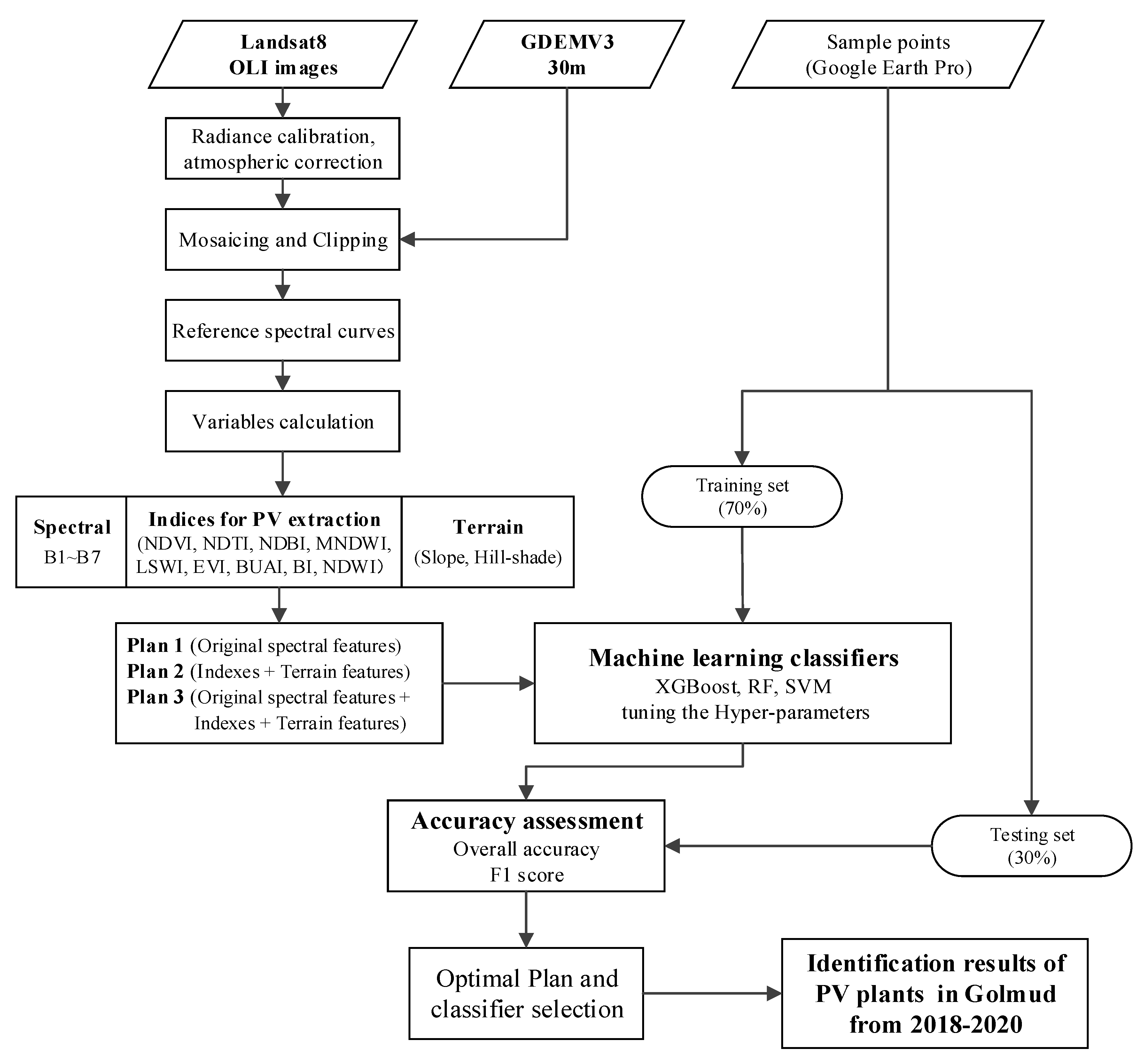
The approach pursued in the present study is shown as a flowchart in Figure 2. Medium-resolution OLI images and the GDEMV3 were utilized. First, the images were preprocessed using radiation calibration, atmospheric correction, and cropping. Indexes for the extraction of PV plants were then computed, and three plans were set. In Plan 1, unprocessed raw spectral features were utilized. Plan 2 included normalized indices derived from specific band intervals after processing the raw data to highlight or suppress the effects of different factors. 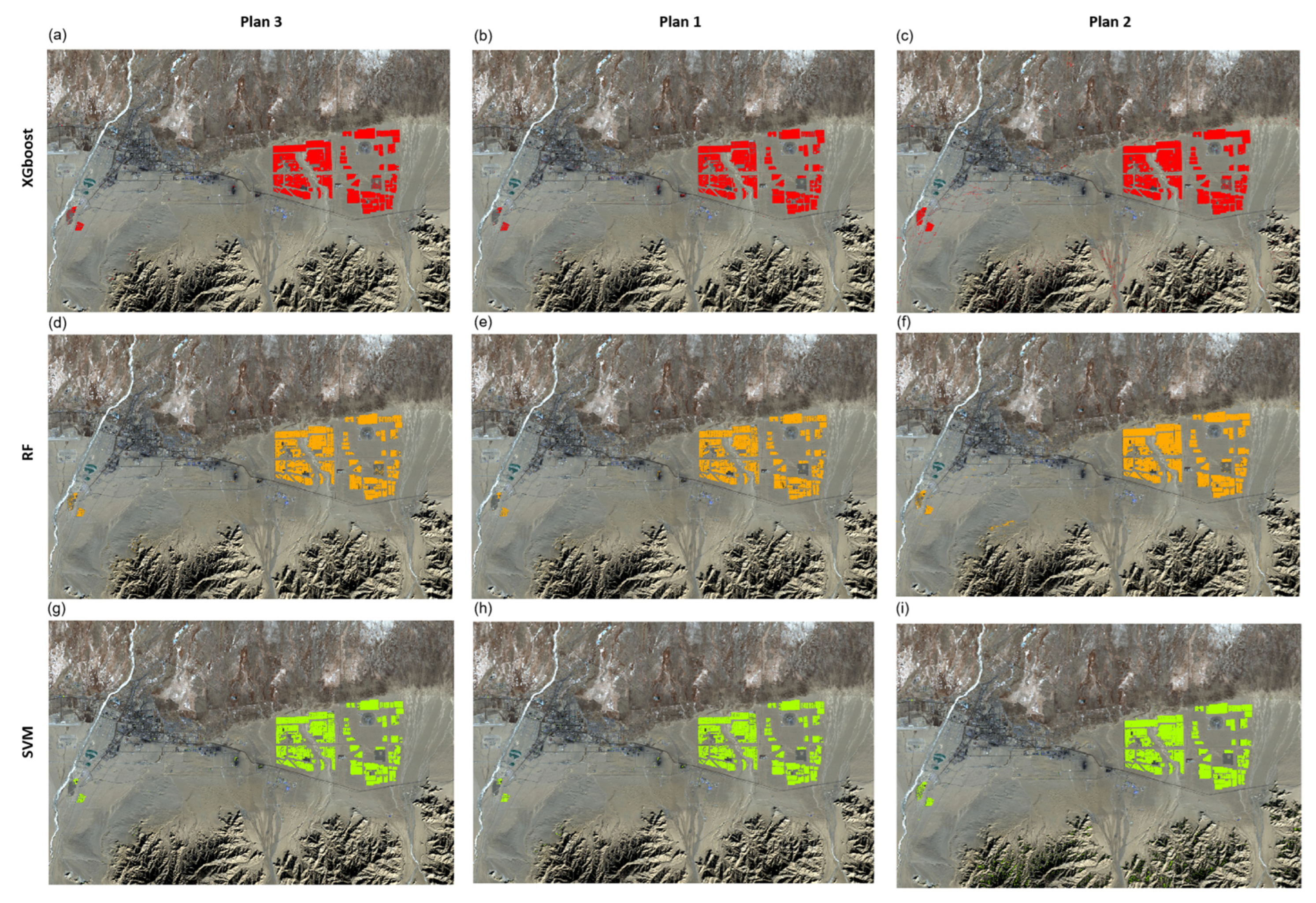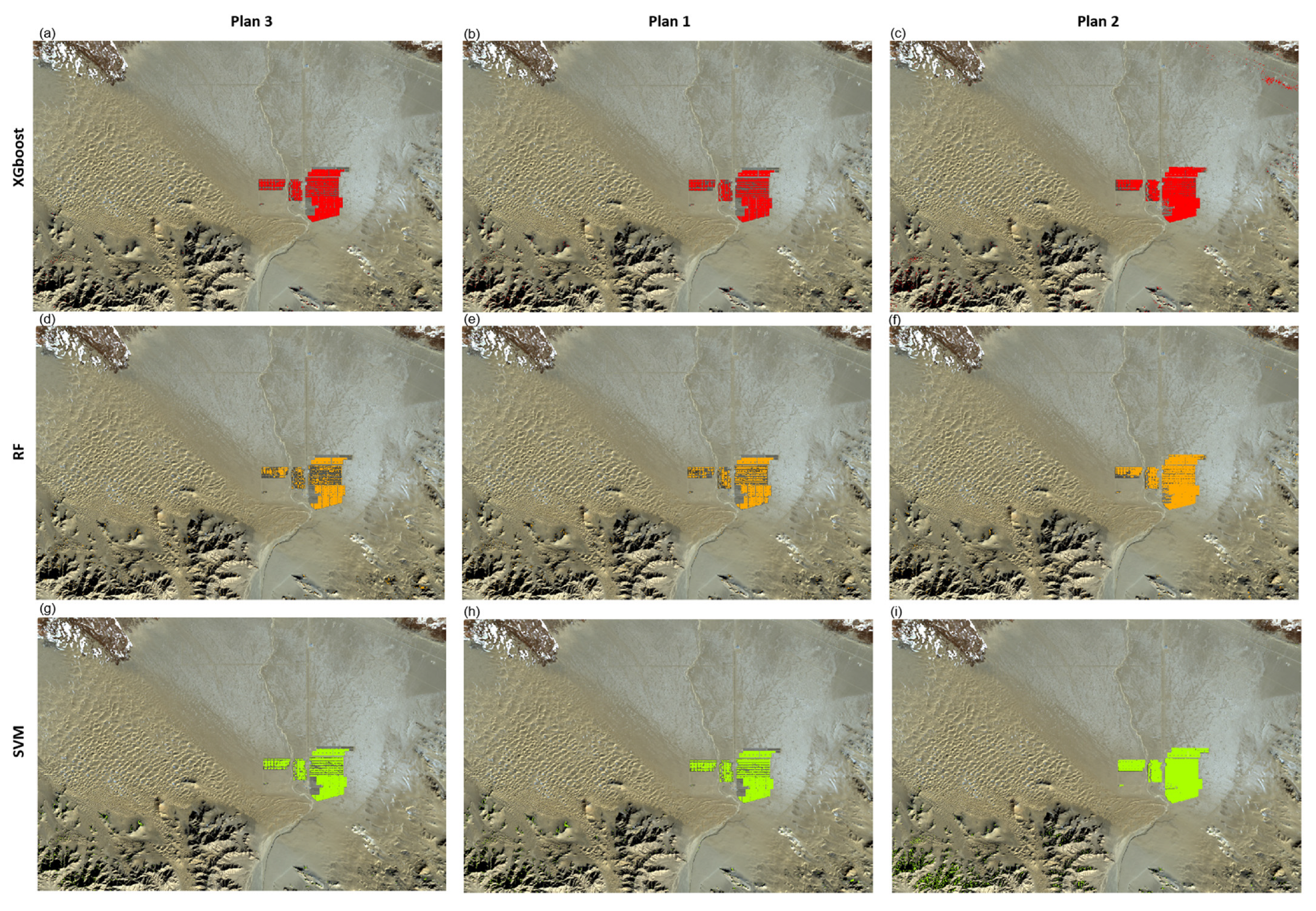Plan 3 used a combination of raw spectral data, index information, and topographic features (Figure 2). In the present study, the performances for the extraction of PV plants using XGBoost, RF, and SVM classifiers were compared using the overall accuracy values and F1 scores. Google Earth Pro was used for the collection of training and test data samples.

3.2. Collection of Training and Test Samples

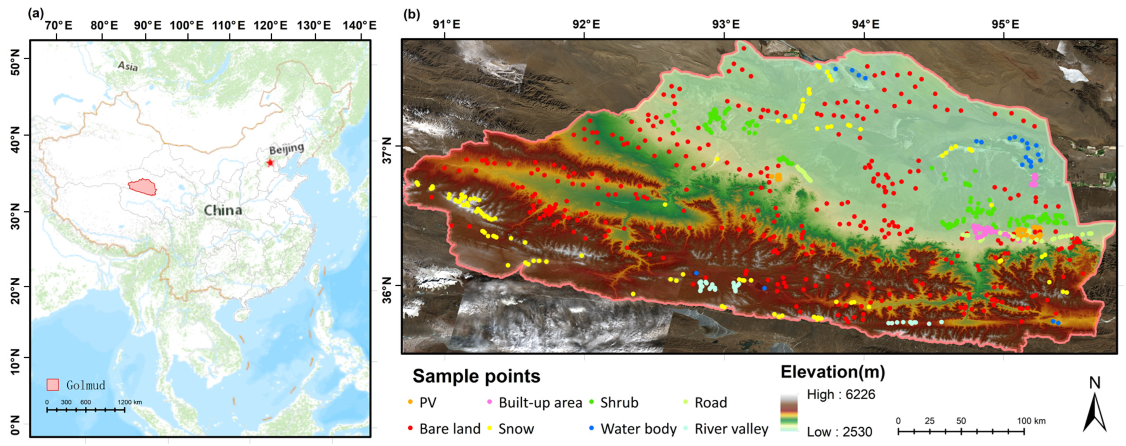
To ensure the accuracy of the classification and the stability of the model, many samples that adequately reflect the parameter space are required. In the present study, based on the distribution of land cover types, attention was devoted to those that are easily confused with PV plants, such as bare land and roads. The land in the area was partitioned into the following categories: Built-up areas, roads, PV plants, bare land, river valleys, shrubs, water bodies, and snow cover.

For specific calibrations at the sample sites, we first used the Global Power Plant Database to target the locations of PV plant construction in the Golmud region. We then used Google Earth Pro to mark 2059 PV sample sites in the study area based on the specific shape and concentrated distribution of PVs, which are easily observed in high-resolution imagery. In the meantime, we carried out a field survey of the selected PV plants and compared the PV sample points on Google Earth with the measured GPS coordinates data to ensure the reliability of the PV sample points and the feasibility of using Google Earth to sample the PV plants. Samples were then collected evenly across carefully selected typical land types in the study area, resulting in a total of 63,323 sample points: PVs (2059), built-up land (1461), roads (397), bare land (41,607, e.g., deserts, semi-deserts, and the Gobi), river valleys (2210), shrubs (965), water bodies (12,830), and snow (1095).

To ensure consistency and robustness, the sample points were selected independently by two technicians with remote sensing backgrounds and then cross-validated. If both agreed, the point was incorporated into the final selection. A third technician was consulted for points that were ambiguous and then discussed until the results of the sample points were agreed upon. We used Google Earth Pro for sample point selection, and contemporaneous historical Landsat8 OLI images were used as references. In addition to visually assessing the accuracy of the sample site selection, we also ensured adequate separation between the sampled features (

Table 1. Classification categories with examples of high-resolution imagery from Google Earth.

Category	Reference Images from Google Earth	Category	Reference Images from Google Earth
PV		Snow
Built-up land		Water body
Road		Shrub
Bare land		River valley

). We calculated the Jeffries–Matusita and Transformed Divergence separability of the ROI using ENVI (all ≥ 1.9), demonstrating the good separation of the sample points [33]. Finally, a stratified random sample of the eight land classes was used to allocate the training and validation datasets, ensuring that 70% of the random samples for each class were used for training, while the remaining 30% were used for validation. The training and validation datasets were evenly distributed throughout the study area, which was conducted using ArcGIS.

3.3. Spectral Characteristics of Confusing Features

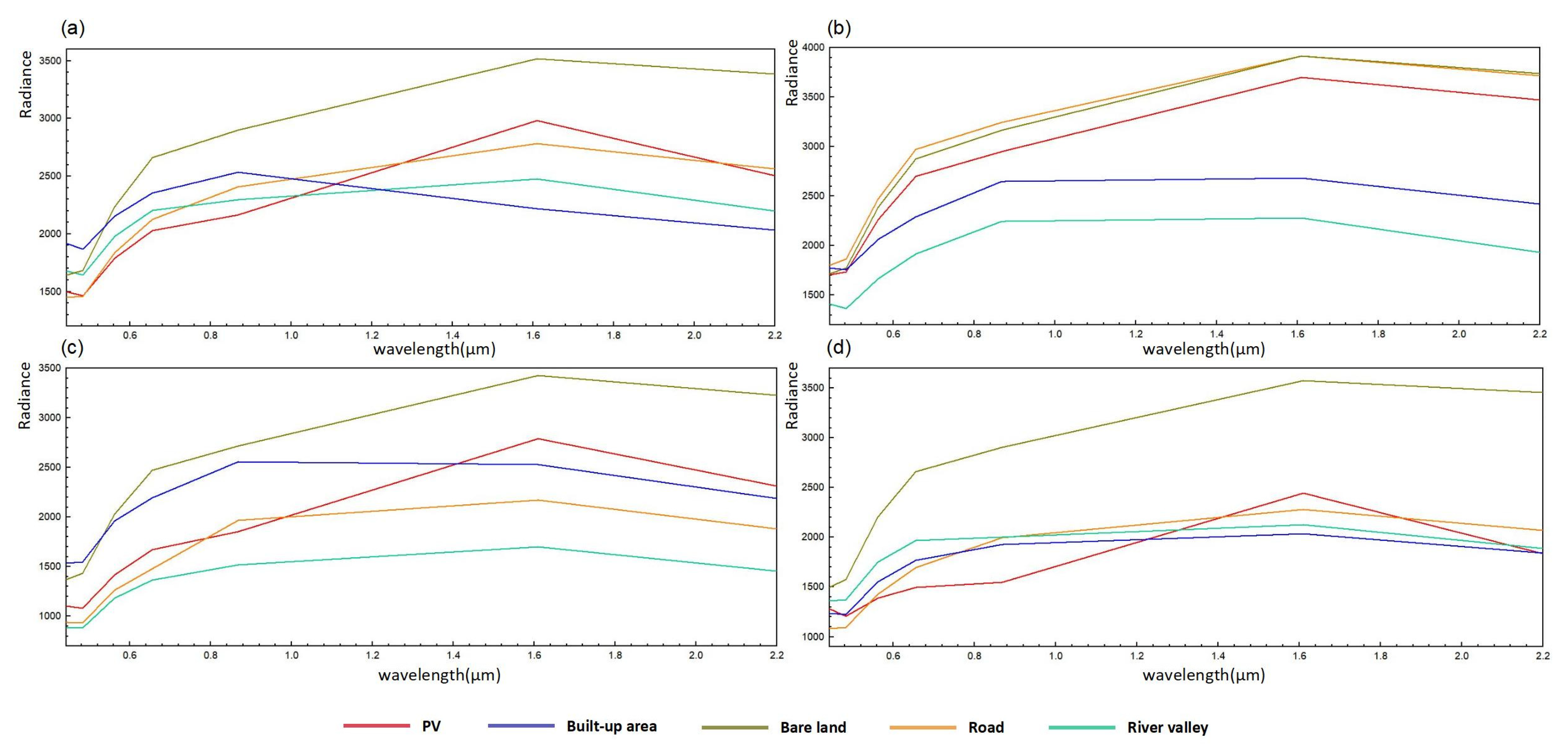
In the present study, PV plants were easily confused with the surrounding bare land (especially between mountain ranges). Spectral curves of land cover types vary according to the spectral reflectance of materials on the surface. Therefore, the surrounding environment, temperature, and land cover types can also cause changes in spectral profiles. Spectral curves of PV plants and land cover types, such as water bodies, snow, and built-up areas significantly differ, and thus, these can be easily distinguished. Those of PV plants and land cover types containing high Si, such as bare land and roads, are similar. However, even though spectral profiles of confusing features exhibit an overall similarity, some differences exist. In particular, the spectral curve of PV plants rises sharply from the near-infrared (NIR) to the short-wave infrared (SWIR) region (0.85–1.65 μm), and it falls significantly in the SWIR region (1.65–2.2 μm).

To evaluate the impacts of seasons on different land cover types, spectral curves were generated for the samples for four months (Figure 3). In general, the curves for PV plants are stable throughout the year, but these plants were distinguished more easily from confusing land cover types in December (winter).

3.4. Selection of Principal PV Extraction Variables

The variables were divided into the following groups: Raw reflectance spectral, PV extraction index, and terrain features (

Table 2. Summary of the categories of variables used to classify PV plants in the study area.

	Variable	Description	Formula	Reference
Spectral	B1	Blue1	B1	[22]
	B2	Blue2	B2
	B3	Green	B3
	B4	Red	B4
	B5	Near-infrared	B5
	B6	Shortwave infrared1	B6
	B7	Shortwave infrared2	B7
Indexes for PV extraction	NDVI	Normalized Difference Vegetation Index	NDVI = (B5 − B4)/(B5 + B4)	[27]
	EVI	Enhanced Vegetation Index	EVI = [2.5 × (B5 − B4)]/(B5 + B6 × 4 − 7.5 × B2 + 1)	[26]
	NDBI	Normalized Built-up Index	NDBI = (B6 − B5)/(B6 + B5)	[29]
	LSWI	Land Surface Water Index	LSWI = (B5 − B7)/(B5 + B7)	[23]
	NDTI	Normalized Difference Tillage Index	NDTI = (B6 − B7)/(B6 + B7)	[30]
	NDWI	Normalized Difference Water Index	NDWI = (B3 − B5)/(B3 + B5)	[25]
	MNDWI	Modified NDWI	MNDWI = (B3 − B6)/(B3 + B6)	[24]
	BUAI	Built-up area Index	BUAI = NDBI − NDVI	[31]
	BI	Bare Soil index	SI = (B6 + B4 − B5 − B2)/(B6 + B4 + B5 + B2)	[28]
Terrain	Slope	Slope	Slope	[32]
	Hill-shade	Hill-shade	Hill-shade

). The raw reflectance spectral variables comprised seven bands including the aerosol, blue, green, red, and NIR as well as two SWIR (1 and 2). The nine indexes associated with PV plants extraction (NDVI, EVI, NDBI, LSWI, NDTI, NDWI, MNDWI, BUAI, and BI) were selected by observing changes in the spectral curves (Figure 3). These indexes are sensitive to changes in the PV plants, surrounding vegetation, soil, built-up areas, impervious surfaces, water bodies, and bare ground. The terrain variables, such as the slope and hill-shade, were calculated using the ASTER GDEM elevation data with a resolution of 30 m.

To highlight the effects of different features on the identification of PV plants, three experimental schemes (Plans 1, 2 and 3) based on features were designed (

Table 3. Categories involved in the experimental schemes.

Experimental Scheme	Feature
Plan 1	original spectral
Plan 2	indexes + terrain
Plan 3	original spectral + indexes + terrain

). In Plan 1, the original spectral features were utilized, and thus, it involved all band values. Conversely, Plan 2 comprised normalized indexes derived from specific band intervals after processing the original data to highlight or suppress the impact of different factors. Plan 3 is a combination of the original spectral and index information as well as terrain features, and thus, it is associated with the most information. Owing to the relatively coarse resolution of OLI imagery, the widths of and distances between PV panels are within a few meters, and textures are almost undetectable. Therefore, the inclusion of textures minimally enhanced the accuracy of the model.

3.5. Machine Learning Models

In the present study, the XGBoost, RF, and SVM models were tested for the identification of PV plants, and their performances were compared. The SVM model is mainly used to solve problems based on the optimization theory. This approach principally involves finding a hyperplane, such that a sub-hyperplane adequately separates data points of two classes and ensures the separated data points of both classes are furthest from the classification plane. Consequently, the SVM model is characterized by a good generalization capability for classification problems. Moreover, in SVM models, kernel functions can be utilized for nonlinear classifications [34]. Conversely, an RF model is a collection of decision trees based on bagging techniques, and it involves the construction of several decision trees from a random subset of the training data [35]. Therefore, the RF model produces good results in feature-based classifications [36], and it is the most effective model for the recognition of features from remote sensing data using the Google Earth Engine (GEE) [37]. The XGBoost is a recently proposed advanced decision-tree gradient-boosting framework. This classifier involves multi-threading of the central processor and the introduction of regularization terms, which are mainstream in popular machine learning schemes [21]. This model has shown high performance in the identification of crops, and it is described as superior to some deep learning models [20]. The XGBoost model runs fast and involves high computational accuracy and low complexity. However, to date, no large-area pixel-based recognition of PV plants has been reported using this model.

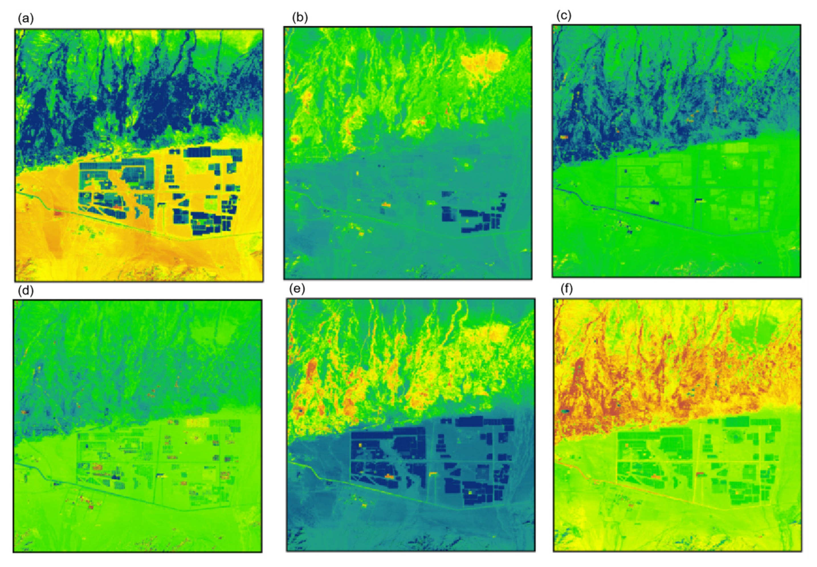
To compare the performance of the three machine learning classifiers, the Python packages “XGBoost” (https://xgboost.readthedocs.io/en/latest/python/index.html, accessed on 24 December 2021) and “Scikit-learn” (https://scikit-learn.org/stable/index.html, accessed on 24 December 2021) were used to process the remote sensing images. The processing of the OLI images, evaluation of the DEM datasets, and raster calculation of normalized indexes were performed using ENVI 5.3 (Figure 4). During the development of the classification model, hyperparameters (

Table 4. Summarized data for hyperparameters for three machine learning classifiers.

Classifier	Hyperparameter	Candidate Values (X0, Xn, i)	Plan 1	Plan 2	Plan 3
XGBoost	n_estimators	(10, 510, 20)	310	310	310
	subsample	(0.7, 1, 0.01)	0.95	0.97	0.95
	eta	(0, 0.30, 0.01)	0.12	0.13	0.11
	gamma	[0.05, 0.1, 0.2, 0.3, 0.5, 0.7, 1, 2, 3, 5, 7, 10] *	0.05	0.05	0.05
	max_depth	(2, 50, 2)	15	15	12
	colsample_bytree	(0.7, 1, 0.01)	0.97	1	0.93
	lambda	[1] *	1	1	1
	alpha	[0] *	0	0	0
RF	n_estimators	(10, 510, 20)	270	190	210
	max_depth	(2, 50, 2)	18	18	16
	min_samples_leaf	[1, 2, 5, 10, 15, 20, 30, 50] *	1	1	1
	min_samples_split	[2, 5, 10, 15, 20, 30, 50] *	2	2	2
	max_features	[‘log2′, ‘sqrt’, None] *	sqrt	sqrt	sqrt
SVM	C	[0.1, 0.3, 1, 3, 10, 30, 100] *	1	5	5
	gamma	[‘auto’] *	auto	auto	auto

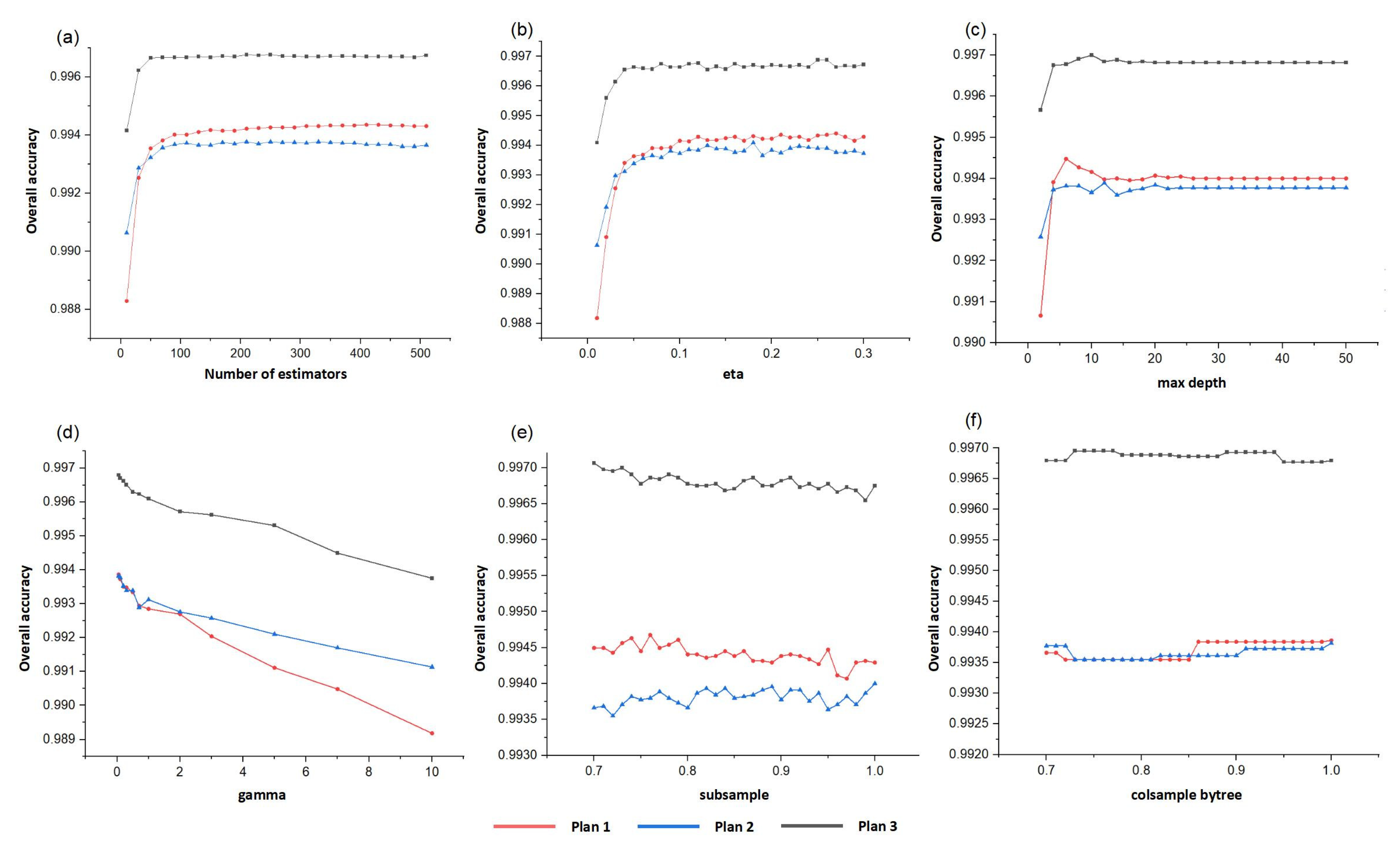
* X₀ is the initial value, X_n denotes the final value, i represents the step size, and [] * stands for all values that can be selected. The naming of all parameters follows rules documented for the corresponding software packages.

) must be configured for each classifier. A combination of “grid search” and “learning curve” strategies was utilized to optimize and select the best values of the main hyperparameters for a chosen classifier (Figure 5 and Figure 6), and the classifier was trained via several iterations. Considering that the performance of a classifier is mainly controlled by the subset of hyperparameters, a grid search improves the efficiency of the hyperparameter optimization according to test results.

The parameters were adjusted by selecting the training set (70%), and the objective function was the overall accuracy (OA). To eliminate the effect of sample selection on the results for a model, cross-validation associated with stratified random sampling (k = 5) was utilized for the parameter evaluation. The accuracy of each model was the average overall accuracy of five tests.

Considering that the grid search is an exhaustive method, parameter optimization can be performed using the GridSearchCV module in the “Scikit-learn”. However, the model in the present study involved many hyperparameters, and because of limitations in the computing power, a one-on-one optimization strategy was adopted. After many experiments, we optimized each of the models (Table 4). After a parameter was optimized, the optimal value was transferred to the next step in the optimization process, thereby traversing all parameters (Table 4; Figure 5 and Figure 6). This parameter was then chosen as the highest OA value in the relative stability interval.

To optimize the performance of the XGBoost model, parameters of the n_estimators, subsample, eta, gamma, max_depth, etc. were tuned. First, we adjusted the three important hyperparameters of the integration algorithm itself: “n_estimators”, “subsample”, and “eta”. The “n_estimators parameter” is the number of weak estimators in the integration, which must be adjusted first. The “subsample” controls the random sampling, and in each put-back process, the weight of samples that were misjudged by a previous tree increases. The new decision tree then favors the samples with higher weights that are likely to be judged incorrectly, and this elevates the accuracy of the model. The “eta” is the step size (also known as the “learning rate”) process of an iterative decision tree. The higher the value of the eta, the faster the iteration; however, this is associated with the risk of non-optimal convergence. In contrast, the lower the value of eta, the higher the chance of finding the best value; however, the iterations may be slower. Therefore, to select an appropriate eta, a trade-off is necessary. In gradient boosting, the “gamma” is a regularization hyperparameter that controls complexity, and thus, it is an influential parameter in XGBoost. Therefore, as the gamma increases, the regularization also increases, and the algorithm becomes more conservative. The “max_depth” determines the maximum number of end nodes in the leaves of trees (Figure 5). These hyperparameters were calculated based on the grid search and cross-validation in Python, and the best results after tuning using the XGBoost are presented in Table 4.

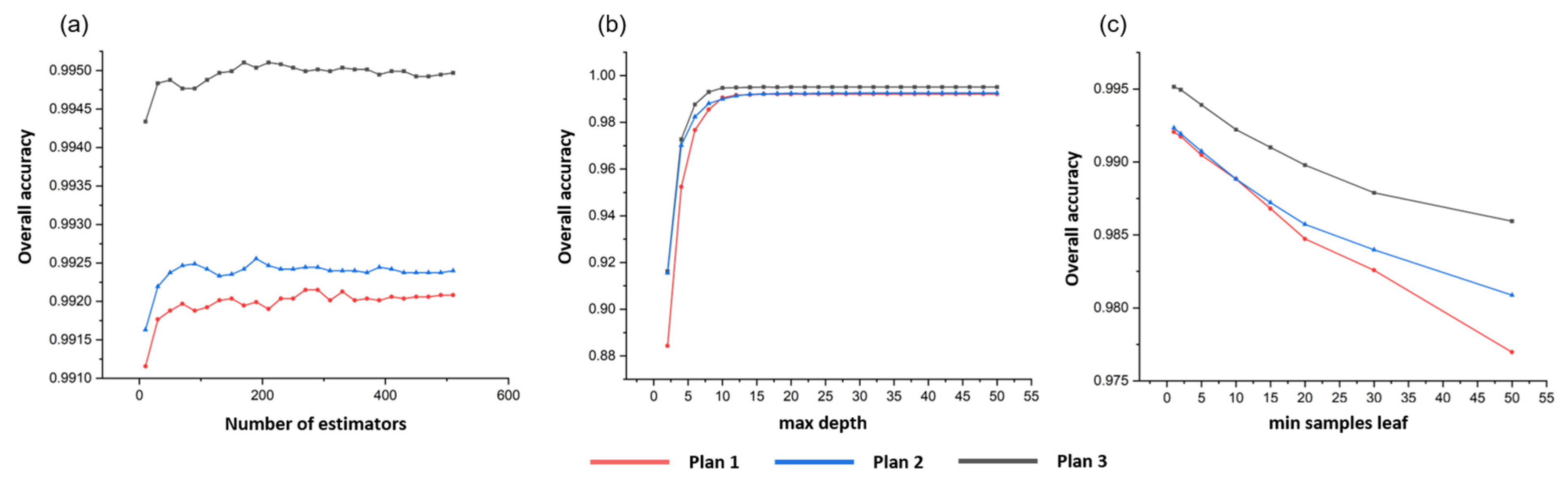
We also adjusted the parameters of the RF and SVM models. Larger n_estimators values indicate that the model learns more and that it is easier to over-fit in RF. Therefore, n_estimators was the first parameter tuned in the RF model, and the remaining parameters were tuned in a similar way for XGBoost (Figure 6). In the adopted SVM model, the radial basis function kernel (RBF) produced an outstanding performance. The model was optimized using the hyperparametric “gamma” and “C” (cost) to address nonlinearity and overfitting. The optimal model was obtained using limited computational power, and the results were satisfactorily validated.

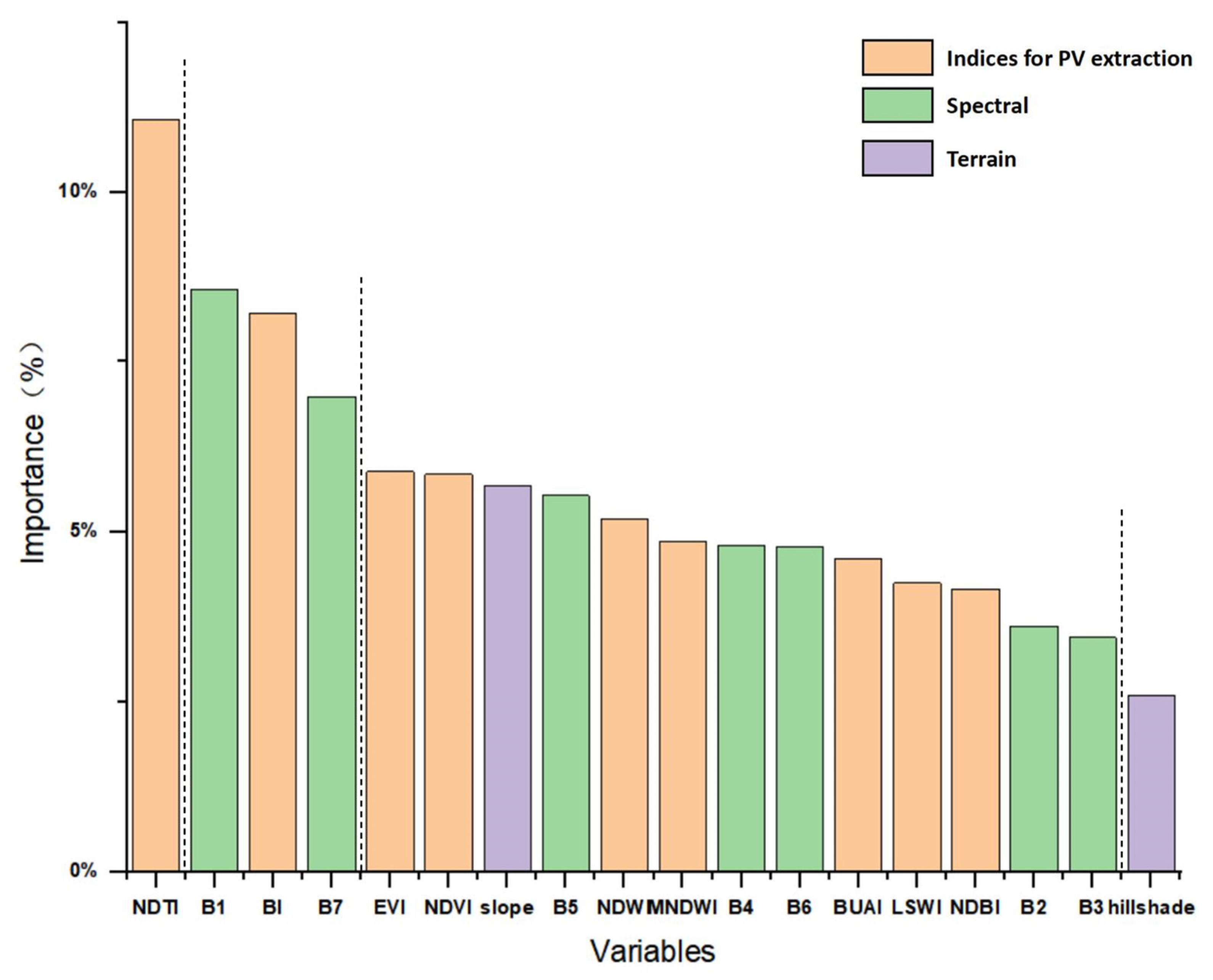
In addition, the XGBoost algorithm can be used to retrieve the importance scores of the variables, thereby obtaining the importance ranking of the independent variables. When more variables are used for key decisions in the decision tree, the relative importance score is higher. This importance score is calculated explicitly for each variable in the dataset, allowing the variables to be ranked and compared. The key influences for the simulation were filtered by calculating and ranking the importance of independent variables using the XGBoost algorithm [38]. The independent variable importance (Equation (1)) was calculated as follows:

$$F_{\left(X\right)}=\frac{x_i}{{{\displaystyle \sum }}_1^n{x}_i} \left(i\in \left[1,n\right]\right).$$

(1)

where x_i denotes the characteristic information gain.

3.6. Model Evaluation

First, a confusion matrix was constructed, and the overall accuracy (Equation (2)) was calculated. The Macro F1 score (Equation (4)) was then used to evaluate the performance of the three classifiers.

The OA is an important parameter for testing the accuracy of a model. In the present study, it was used to assess the model by evaluating the proportion of correctly classified samples relative to all samples, and this is expressed as follows:

$$OA= \frac{TP+TN}{TP+FN+FP+TN}.$$

(2)

Regarding each class, the F1 score was co-determined using the producer and user precision values as follows:

$$F{1}_{class i}= \frac{2}{\left(\frac{1}{P{A}_{class i}}+\frac{1}{U{A}_{class i}}\right)}.$$

(3)

whereas the Macro F1 score, which represents the average result of all classes, was calculated as follows:

$$Macro F1 score=\frac{1}{n}{\displaystyle {{\displaystyle \sum }}_1^n}F{1}_{class i}(i\in [1,n]).$$

(4)

In the test set, an accuracy of 1% corresponded to an area of approximately 17 km².

3.7. Image Post-Processing

As the target subject was concentrated PVs, the PV pixels were centrally distributed, and no isolated pixel points were present. We therefore used 3 × 3 median filtering to eliminate isolated noise points after classification. Median filtering is a non-linear smoothing technique in which the value of each pixel is replaced by the median of the values of all pixels in a neighborhood window such that the surrounding pixel values are similar to the true value, thereby eliminating isolated noise points [39].

4. Results

4.1. Model and Plan Comparison and Selection

Following the determination of the appropriate hyperparameters for each model, the remaining 30% of the test data were utilized to identify PV plants in each of the nine experimental plans (i.e., three classifiers × three plans), and the impacts of the different variables on the performance of the models were further evaluated (

Table 5. Data for the overall accuracy and macro F1_score (in brackets) associated with different classification experiments.

OA	Plan 1	Plan 2	Plan 3
XGBoost	99.37% (0.9412)	99.47% (0.9458)	99.65% (0.9631)
RF	99.23% (0.9253)	99.12% (0.9292)	99.47% (0.9499)
SVM	97.94% (0.7988)	98.43% (0.8569)	98.32% (0.8405)

).

The XGBoost model is superior to those of the RF and SVM, irrespective of the plan, and this produced the highest OA (99.65%) and F1_score (0.9631). The best accuracy values achieved using the RF and SVM models are 99.47% and 98.32%, respectively.

The results also reveal that the performances of the XGBoost and RF models are improved (higher OA and Macro F_scores) under Plan 3 compared to those under Plans 1 (spectral only) and 2 (PV extraction indices and terrain). Regarding the SVM model, the highest accuracy was obtained under Plan 2 instead of Plan 3. Variations in the macro F1_score exhibit a trend similar to that for the OA value. Moreover, the results indicate that a combination of the spectral, index, and terrain features provides adequate data for the identification of PV plants, and thus, a classification characterized by a better accuracy compared to those based on texture features utilized in a previous study was achieved [18].

To enhance the display of the classification results based on various models, two representative PV plants in the east and center of Golmud City and the surrounding complex terrain were utilized to show the classification for 2020 (Figure 7 and Figure 8).

The PV identification results for two areas were compared using high-resolution images obtained from the GEE for the same period. In Plan 1, the pixels attributed to PV plants are adequately separated from the surrounding area, bare land, and vegetation. However, some associated pixels within the PV plant (e.g., buildings, concrete surfaces, PV panels, and roads) were missed. In fact, many PV panels were regarded as concrete and roads, and thus, these were not identified (Figure 7). In Plan 2, PV extraction indexes and terrain features were utilized for the extraction of information within PV plants; however, the associated misclassification is even higher. This is because, within the PV plants, concrete surfaces and buildings were commonly extracted as PV pixels (Figure 8). Concurrently, misclassified pixels attributed to PV plants are numerous in the mountains, bare land, and river valleys in the northwest corner of the images.

Areas occupied by PV plants in both sites were also calculated (

Table 6. Calculated areas occupied by PV plants in Site 1/Site 2 based on different models and plans (unit: ha).

Area1/ha	Plan 1	Plan 2	Plan 3
XGBoost	5552.1/1018.71	6949.44/2598.21	5934.78/1085.13
RF	5349.78/1035.72	6480.81/1974.06	5496.39/1022.13
SVM	5568.03/1340.55	6811.74/2698.74	5644.8/1241.01

).

Table 7. Confusion matrix of the highest overall accuracy classifications.

Category	PV	Bare Lands	Built-Up Areas	Snow Cover	Shrubs	Water Bodies	Roads	River Valleys	Total	User’s Accuracy
PV	617	0	0	0	0	0	1	0	618	99.84%
Bare lands	1	12479	0	0	0	0	2	0	12,482	99.98%
Built-up areas	2	0	428	0	3	0	4	1	438	97.72%
Snow cover	0	0	1	327	0	0	0	0	328	99.70%
Shrubs	0	2	1	0	286	0	0	0	289	98.96%
Water bodies	0	0	0	0	0	3849	0	0	3849	100.00%
Roads	1	18	18	0	0	0	74	0	111	66.67%
River valleys	0	5	7	0	0	0	0	869	881	98.64%
Total	621	12504	455	327	289	3849	81	870	18,996
Producer‘s Accuracy	99.36%	99.80%	94.07%	100.00%	98.96%	100.00%	91.36%	99.89%
Overall Accuracy (OA): 99.65% macro F1_score: 0.9631

shows the confusion matrix with the highest overall PV extraction accuracy (XGBoost, Plan 3). The table indicates that the land types most confused with PV were bare land, built-up areas, and roads; however, the overall classification accuracy reached 99.65%, the macro F1_score reached 0.9631, and the user (99.84%) and producer accuracies (99.36%) for PV extraction were above 99%, which generally meets the requirements of PV thematic information extraction.

4.2. Influence of Variables on the Model

Following the determination of the optimal model and plan, the impact of each variable on the performance of the model was evaluated, using the XGBoost model. The 18 variables in the three categories contributed variably to the extraction of the PV plant (Figure 9). Overall, the variable importance can be divided into four levels, with a substantial span between the levels. The first level is NDTI (>10%), followed by B1, BI, and B7 (~7.5%), and the third level is EVI-B3 (~5%) and hillshade (~2.5%). As OLI remote sensing imagery was used in this study, the number of bands was small, and nine indices were pre-selected based on their specific roles. Only 18 variables were constructed, which did not affect the model calculations enough to make the data redundant. Although hillshade was the least important variable, it was retained because concentrated PVs in the study area are generally located on plains with low slopes, and the hillshade variable is used to distinguish between confusing mountainous areas and plain areas.

Indexes associated with the extraction of PV plants displayed distinct effects, and the importance of the NDTI, BI, EVI, and NDVI were ranked first, third, fifth, and sixth, respectively. In addition to these four indices, the top three variables for individual reflectance spectra are B1, B7, and B5, which overall ranked second, fourth, and eighth, respectively. These results are consistent with those of previous studies and the patterns exhibited by the spectral curves in Figure 8. The slope variable ranked seventh in importance, and this indicates a topographic influence on the location of PV systems. Flat areas characterized by gentle slopes are suitable for the construction of PV plants, whereas, in areas with steep slopes, the installation and maintenance of PV panels are challenging.

4.3. Extraction of PV Plants in Golmud City

PV plants in Golmud City were extracted and mapped using the XGBoost model associated with Plan 3 because it yielded the highest accuracy (Figure 10). PV plants are concentrated in the three parts of the city, as demonstrated using enlarged images of the specific regions enclosed in small rectangles in Figure 9. Obviously, some areas near the PV plants were misclassified, especially in relatively concentrated regions. Accordingly, a median filter was used to remove these points to eliminate random errors. The calculated extracted area occupied by PV plants in the Qaidam Basin of Golmud City was approximately 10,715.85 ha (107.16 km²).

The identification of PV plants in the east of Golmud City in 2018 and an analysis of the construction of PV plants from 2018 to 2020 were also conducted. The extraction results reveal that the area covered by PV plants increased from 5344.2 ha in 2018 to 5879.34 ha in 2020 (Figure 11). As a pilot energy city, Golmud exhibits the highest density of PV plants in the world. In 2018, 90 grid-connected PV projects involving a capacity of 2804 MW had been completed in the city. Additional PV power projects were ongoing in the city, and 12 were earmarked for completion by the end of 2020.

5. Discussion

5.1. PV Extraction Model

In the classifications of the eight land cover types, higher accuracy values were obtained using the XGBoost model relative to those obtained using the SVM and RF models. The XGBoost model improved the accuracy by iteratively elevating the loss residuals [21]. Thus, the weights of incorrect sample points were enhanced in successive iterations, and incorrectly learned information was reinforced. Therefore, the XGBoost model produced an optimal performance for land cover classification, and the performance improved as the input data changed from Plan 1 to Plan 3. In contrast, the SVM model, which is a binary scheme for building hyperplanes to achieve classification, was less effective when multiple data sources were incorporated. In addition, the performance of the SVM model was substantially affected by mixed pixels and/or mislabeled training samples. This model was more sensitive to noisy data compared to the other algorithms [40], and the accuracy decreased for the three data categories under Plan 3.

The results presented herein, particularly those for the XGBoost model, indicate the superiority of the method, compared to previous studies in Ningxia and Gansu [18,19]. In terms of accuracy, the PV extraction accuracy was substantially improved. The Gansu study used the SVM model and obtained an overall accuracy of 91.39%, while the Ningxia study used the RF model and obtained an accuracy of 98.47%, both of which were lower than the results obtained in this study (99.65%). This study also built on previous research by discarding texture features, which have little influence, and focused on the spectral features of PVs. We were unable to identify interpolated texture features of PVs using medium-resolution images, which reduced the complexity of the model [18]. In addition, previous studies have not tuned the model hyperparameters [19], while we improved the algorithm in this study to maintain very good extraction accuracy, even when the study area was expanded to 71,298.7 km². In contrast, previous studies that used local machines were limited to the areas around the PV plant.

Some researchers have used deep learning methods, including convolutional neural networks (CNNs) and recurrent neural networks (RNNs), to extract PV plants worldwide, using over 10⁶ CPU hours and 20,000 GPU hours, which actually took nearly 2 months [3]. Other researchers have also proposed a PV recognition workflow, but the process of visual interpretation alone has been labor-intensive and time-consuming (the team spent dozens of hours of visual interpretation work filtering the misclassification regions with commission error) [41]. In our study, satisfactory results were achieved using only a local machine (AMD Ryzen™ 9 5950X 16-core 32-thread), computing for approximately 25 h.

5.2. The Importance of Spectral Characteristics on the XGBoost Model to Extract PV PLANTS

The spectral curves of different features were utilized to analyze the differences between areas hosting PV plants and the surrounding land cover types. PV plants can be easily distinguished from other features, including water bodies, snow, vegetation, and built-up areas, owing to the large differences in their spectral shapes. However, the spectral shapes of PV plants are more similar to those of surrounding bare land and river valley roads. Consequently, distinguishing between these features using the overall waveform is impossible. Owing to the strong absorption of crystalline silicon (C-Si), which is a basic component of PV cells, the PV modules produce low reflectivity values in the visible (VIS) range. The absorption decreased between 0.99 and 1.15 μm, which is reflected by a rapid decrease between bands 6 and 7 compared to the other features [42]. The NDTI, which captures this feature, is crucial for identifying PV plants. The BI was used to distinguish PV panels from the surrounding bare land, while the NDVI and EVI were used to identify vegetation. The BUAI, which is used to identify built-up areas in detail, can effectively highlight the characteristics of PV panels as special objects, which differ substantially from commonly confused land types. The results demonstrate that medium-resolution OLI imagery is suitable for investigating the dynamics of clustered PV plants. Considering the lower acquisition cost, lower computation requirements, suitability for long-term retention of the imagery, and the fact calculations can be conducted in a Python environment, the approach proposed herein can be extended to larger spatial areas and longer time scales. However, the medium-resolution OLI imagery provides high accuracy for relatively small areas, owing to the data availability and low processing time [15]. As a result of the coarser resolution of OLI imagery, clustered PV plants are easily identified, even though the identification of distributed PV panels remains challenging [42,43]. Meanwhile, because of the release of PV plant datasets, high-quality training data for models are readily available [44].

This study did have some limitations, including the small number of bands used in the OLI imagery, particularly the lack of detail in the NIR–SWIR interval, which plays an important role in PV extraction, the small number of indices that can be selected, and the limited information obtained from these parameters. Further research should experiment with additional wavelengths and higher-resolution remote sensing images for extraction. In addition to medium-resolution OLI imagery, high-resolution multi-spectral imagery (e.g., Sentinel-2 images) are suitable for distinguishing PV plants from other ground objects [45].

6. Conclusions

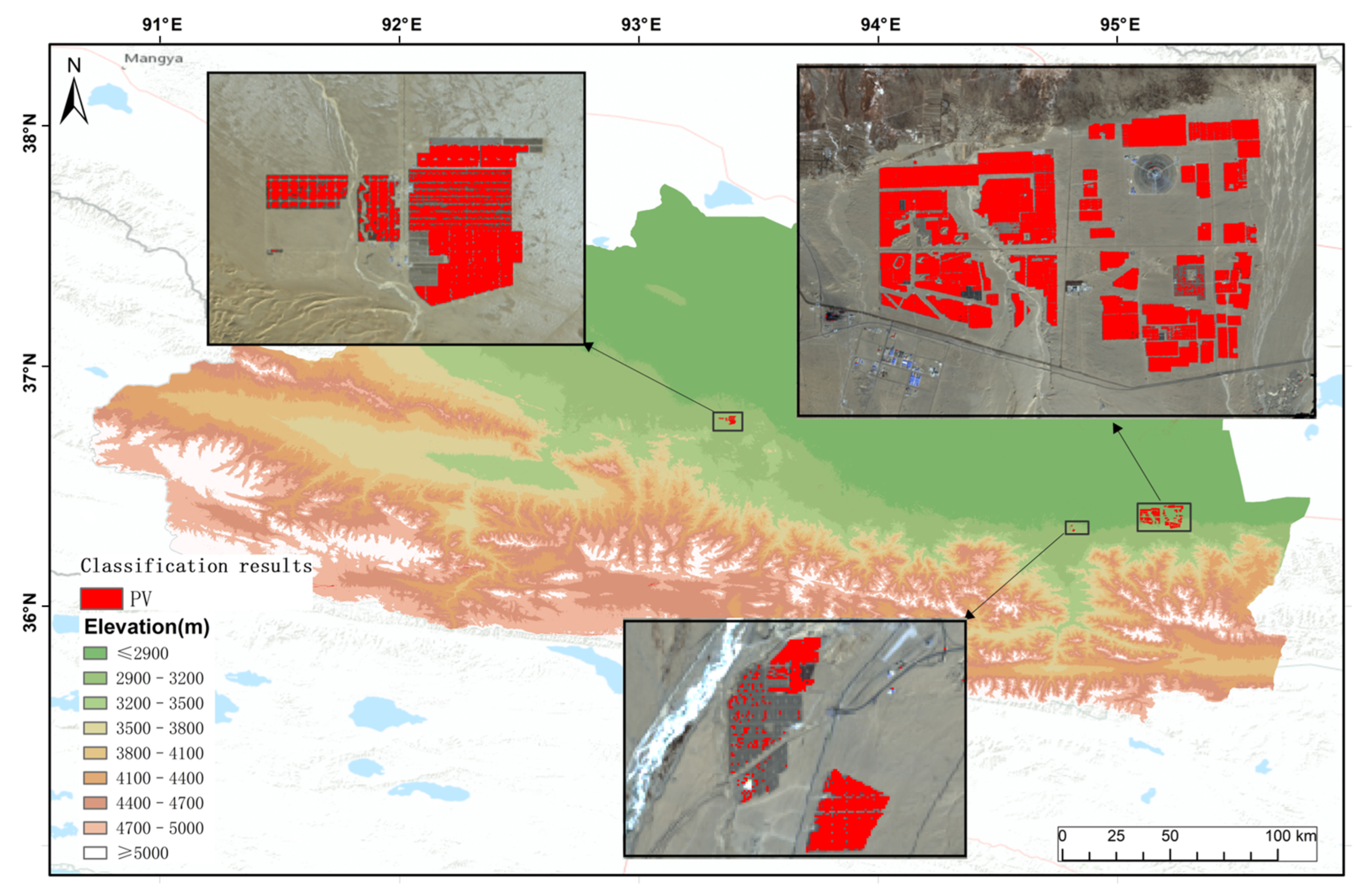
In the present study, PV extraction models were established using indexes, such as the NDTI, BI, NDVI, BUAI, NDWI, etc., and terrain variables. A scheme integrating original spectral features, PV extraction indexes, and terrain features provided optimum results. High-performance machine learning algorithms were combined with the PV extraction models and utilized to compare the performance of the XGBoost, RF, and SVM algorithms. The XGBoost model produced the highest accuracy ((OA = 99.65%, F1score = 0.9631) for a raster-based extraction of PV plants using OLI imagery involving a resolution of 30 m. This approach reduces the reliance on high-resolution imagery and high-performance computers during the extraction of PV plants from satellite imagery.

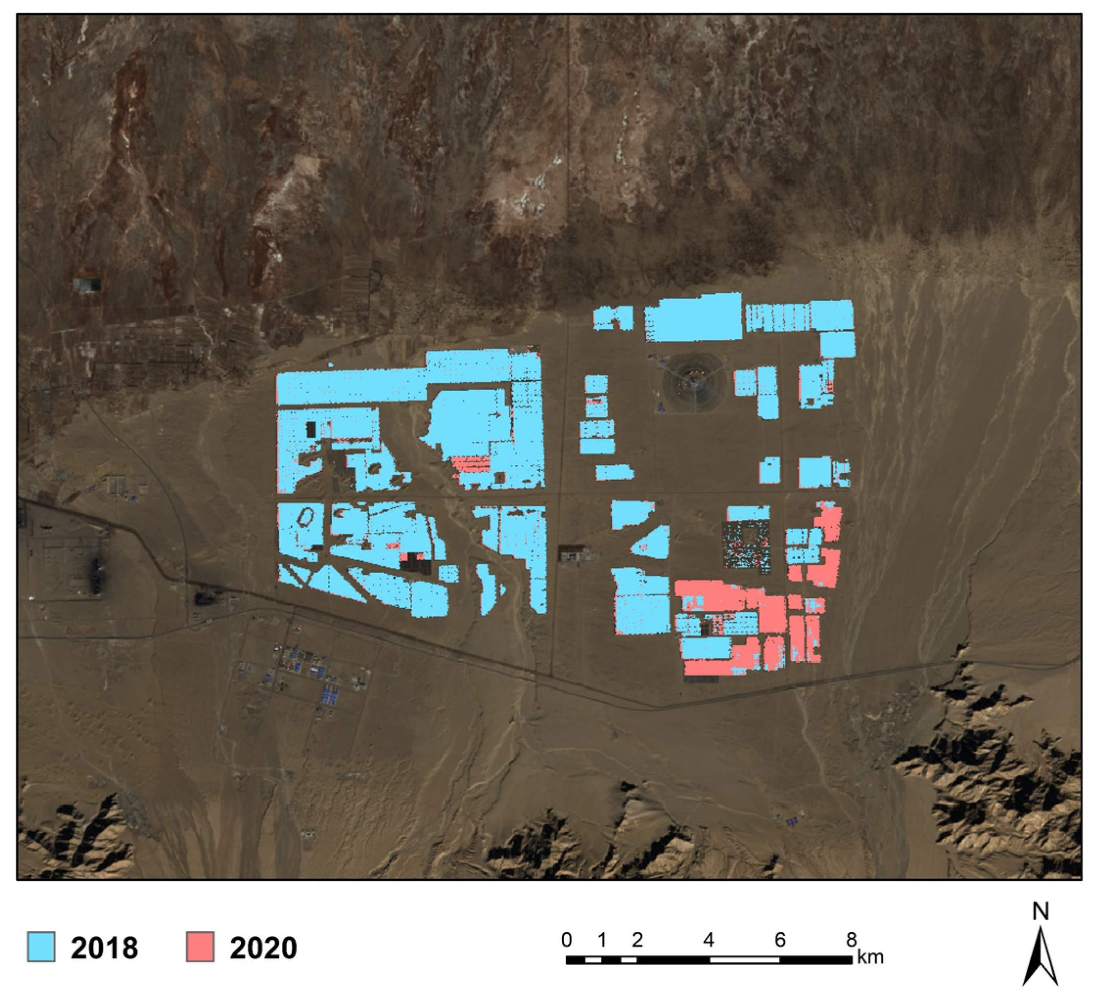
The calculated area occupied by PV plants in the Golmud region in 2020 was 10,715.85 ha. A comparison of the area associated with PV plants in the east of the region based on 2018 imagery revealed an increase of 10% from 2018 (5344.2 ha) to 2020 (5879.34 ha), and this demonstrated the robustness of the proposed approach. The present study represents the foundation for future studies involving longer durations and larger areas.

References

1. Parida, B.; Iniyan, S.; Goic, R. A review of solar photovoltaic technologies. Renew. Sustain. Energy Rev. 2011, 15, 1625–1636. [Google Scholar] [CrossRef]
2. Li, Y.; Nie, D.; Zhao, X.; Li, Y. Market structure and performance: An empirical study of the Chinese solar cell industry. Renew. Sustain. Energy Rev. 2017, 70, 78–82. [Google Scholar] [CrossRef]
3. Kruitwagen, L.; Story, K.T.; Friedrich, J.; Byers, L.; Skillman, S.; Hepburn, C. A global inventory of photovoltaic solar energy generating units. Nature 2021, 598, 604–610. [Google Scholar] [CrossRef] [PubMed]
4. Sahu, A.; Yadav, N.; Sudhakar, K. Floating photovoltaic power plant: A review. Renew. Sustain. Energy Rev. 2016, 66, 815–824. [Google Scholar] [CrossRef]
5. Johansson, B. Security aspects of future renewable energy systems–A short overview. Energy 2013, 61, 598–605. [Google Scholar] [CrossRef] [Green Version]
6. Mackay, D.J.C. Solar energy in the context of energy use, energy transportation and energy storage. Philos. Trans. R. Soc. Lond. Ser. A Math. Phys. Eng. Sci. 2013, 371, 20110431. [Google Scholar] [CrossRef]
7. Scheidel, A.; Sorman, A.H. Energy transitions and the global land rush: Ultimate drivers and persistent consequences. Glob. Environ. Chang. 2012, 22, 588–595. [Google Scholar] [CrossRef]
8. Capellán-Pérez, I.; de Castro, C.; Arto, I. Assessing vulnerabilities and limits in the transition to renewable energies: Land requirements under 100% solar energy scenarios. Renew. Sustain. Energy Rev. 2017, 77, 760–782. [Google Scholar] [CrossRef] [Green Version]
9. Zhang, X.; Xu, M. Assessing the Effects of Photovoltaic Powerplants on Surface Temperature Using Remote Sensing Techniques. Remote Sens. 2020, 12, 1825. [Google Scholar] [CrossRef]
10. Liu, Y.; Zhang, R.; Huang, Z.; Cheng, Z.; López-Vicente, M.; Ma, X.; Wu, G. Solar photovoltaic panels significantly promote vegetation recovery by modifying the soil surface microhabitats in an arid sandy ecosystem. Land Degrad. Dev. 2019, 30, 2177–2186. [Google Scholar] [CrossRef]
11. Broadbent, A.M.; Krayenhoff, E.S.; Georgescu, M.; Sailor, D.J. The Observed Effects of Utility-Scale Photovoltaics on Near-Surface Air Temperature and Energy Balance. J. Appl. Meteorol. Clim. 2019, 58, 989–1006. [Google Scholar] [CrossRef]
12. Hosenuzzaman, M.; Rahim, N.A.; Selvaraj, J.; Hasanuzzaman, M.; Malek, A.B.M.A.; Nahar, A. Global prospects, progress, policies, and environmental impact of solar photovoltaic power generation. Renew. Sustain. Energy Rev. 2015, 41, 284–297. [Google Scholar] [CrossRef]
13. Wu, Z.; Hou, A.; Chang, C.; Huang, X.; Shi, D.; Wang, Z. Environmental impacts of large-scale CSP plants in northwestern China. Environ. Sci. Process. Impacts 2014, 16, 2432–2441. [Google Scholar] [CrossRef] [PubMed]
14. Yu, J.; Wang, Z.; Majumdar, A.; Rajagopal, R. DeepSolar: A Machine Learning Framework to Efficiently Construct a Solar Deployment Database in the United States. Joule 2018, 2, 2605–2617. [Google Scholar] [CrossRef] [Green Version]
15. Castello, R.; Roquette, S.; Esguerra, M.; Guerra, A.; Scartezzini, J.-L. Deep learning in the built environment: Automatic detection of rooftop solar panels using Convolutional Neural Networks. J. Phys. Conf. Ser. 2019, 1343, 012034. [Google Scholar] [CrossRef]
16. Badrinarayanan, V.; Kendall, A.; Cipolla, R. SegNet: A Deep Convolutional Encoder-Decoder Architecture for Image Segmentation. IEEE Trans. Pattern Anal. Mach. Intell. 2017, 39, 2481–2495. [Google Scholar] [CrossRef]
17. Karoui, M.S.; Benhalouche, F.Z.; Deville, Y.; Djerriri, K.; Briottet, X.; Houet, T.; Le Bris, A.; Weber, C. Partial Linear NMF-Based Unmixing Methods for Detection and Area Estimation of Photovoltaic Panels in Urban Hyperspectral Remote Sensing Data. Remote Sens. 2019, 11, 2164. [Google Scholar] [CrossRef] [Green Version]
18. Zhang, X.; Zeraatpisheh, M.; Rahman, M.; Wang, S.; Xu, M. Texture Is Important in Improving the Accuracy of Mapping Photovoltaic Power Plants: A Case Study of Ningxia Autonomous Region, China. Remote Sens. 2021, 13, 3909. [Google Scholar] [CrossRef]
19. Wang, S.L.; Zhang, L.P.; Zhu, S.H.; Ji, L.; Chai, Q.; Shen, Y.; Zhang, R. Extraction of photovoltaic power plants from Landsat 8 OLI remote sensing images by combining multiple common features. Bull. Surv. Mapp. 2018, 46–52. [Google Scholar] [CrossRef]
20. Liheng, Z.; Lina, H.; Hang, Z. Deep learning based multi-temporal crop classification. Remote Sens. Environ. 2019, 221, 430–443. [Google Scholar]
21. Chen, T.; Guestrin, C. XGBoost: A Scalable Tree Boosting System. In Proceedings of the 22nd ACM SIGKDD International Conference on Knowledge Discovery and Data Mining, San Francisco, CA, USA, 13–17 August 2016; pp. 785–794. [Google Scholar]
22. Roy, D.P.; Wulder, M.A.; Loveland, T.R.; Woodcock, C.E.; Allen, R.G.; Anderson, M.C.; Helder, D.; Irons, J.R.; Johnson, D.M.; Kennedy, R.; et al. Landsat-8: Science and product vision for terrestrial global change research. Remote Sens. Environ. 2014, 145, 154–172. [Google Scholar] [CrossRef] [Green Version]
23. Qin, Y.; Xiao, X.; Dong, J.; Zhou, Y.; Zhu, Z.; Zhang, G.; Du, G.; Jin, C.; Kou, W.; Wang, J.; et al. Mapping paddy rice planting area in cold temperate climate region through analysis of time series Landsat 8 (OLI), Landsat 7 (ETM+) and MODIS imagery. ISPRS J. Photogramm. Remote Sens. 2015, 105, 220–233. [Google Scholar] [CrossRef] [PubMed] [Green Version]
24. Xu, H. Modification of normalised difference water index (NDWI) to enhance open water features in remotely sensed imagery. Int. J. Remote Sens. 2006, 27, 3025–3033. [Google Scholar] [CrossRef]
25. Gao, B.-C. NDWI—A normalized difference water index for remote sensing of vegetation liquid water from space. Remote Sens. Environ. 1996, 58, 257–266. [Google Scholar] [CrossRef]
26. Huete, A.; Didan, K.; Miura, T.; Rodriguez, E.P.; Gao, X.; Ferreira, L.G. Overview of the radiometric and biophysical performance of the MODIS vegetation indices. Remote Sens. Environ. 2002, 83, 195–213. [Google Scholar]
27. Tucker, C.J. Red and photographic infrared linear combinations for monitoring vegetation. Remote Sens. Environ. 1979, 8, 127–150. [Google Scholar] [CrossRef] [Green Version]
28. Rikimaru, A.; Roy, P.S.; Miyatake, S. Tropical forest cover density mapping. Trop. Ecol. 2002, 43, 39–47. [Google Scholar]
29. Zha, Y.; Gao, J.; Ni, S. Use of normalized difference built-up index in automatically mapping urban areas from TM imagery. Int. J. Remote Sens. 2003, 24, 583–594. [Google Scholar] [CrossRef]
30. VanDeventer, A.P.; Ward, A.D.; Gowda, P.H.; Lyon, J.G. Using thematic mapper data to identify contrasting soil plains and tillage practices. Photogramm. Eng. Remote Sens. 1997, 63, 87–93. [Google Scholar]
31. He, J.; Liu, X.; Tu, L.; Xu, K.; He, Z.; Song, H.; Liu, H. Automatic extraction of impermeable surface information in Nanchang. Bull. Surv. Mapping 2020, 1–4. [Google Scholar] [CrossRef]
32. Rediske, G.; Siluk, J.C.M.; Gastaldo, N.G.; Rigo, P.D.; Rosa, C.B. Determinant factors in site selection for photovoltaic projects: A systematic review. Int. J. Energy Res. 2018, 43, 1689–1701. [Google Scholar] [CrossRef]
33. Richards, J.A. Remote Sensing Digital Image Analysis; Springer: Berlin, Germany, 1999. [Google Scholar]
34. Dai, A.; Zhou, X.; Wu, Z. Design of an intelligent controller for a grain dryer: A support vector machines for regression inverse model proportional–integral–derivative controller. Food Sci. Nutr. 2020, 8, 805–819. [Google Scholar] [CrossRef] [PubMed]
35. Lawrence, R.L.; Wood, S.D.; Sheley, R.L. Mapping invasive plants using hyperspectral imagery and Breiman Cutler classifications (randomForest). Remote Sens. Environ. 2006, 100, 356–362. [Google Scholar] [CrossRef]
36. Belgiu, M.; Drăguţ, L. Random forest in remote sensing: A review of applications and future directions. ISPRS J. Photogramm. Remote Sens. 2016, 114, 24–31. [Google Scholar] [CrossRef]
37. Blickensdörfer, L.; Schwieder, M.; Pflugmacher, D.; Nendel, C.; Erasmi, S.; Hostert, P. Mapping of crop types and crop sequences with combined time series of Sentinel-1, Sentinel-2 and Landsat 8 data for Germany. Remote Sens. Environ. 2022, 269, 112831. [Google Scholar] [CrossRef]
38. Cao, D.; Ma, Y.; Sun, L.; Gao, L. Fast observation simulation method based on XGBoost for visible bands over the ocean surface under clear-sky conditions. Remote Sens. Lett. 2021, 12, 674–683. [Google Scholar] [CrossRef]
39. George, G.; Oommen, R.M.; Shelly, S.; Philipose, S.S.; Varghese, A.M. A Survey on Various Median Filtering Techniques For Removal of Impulse Noise from Digital Image. In Proceedings of the 2018 Conference on Emerging Devices and Smart Systems (ICEDSS), Tiruchengode, India, 2–3 March 2018; pp. 235–238. [Google Scholar] [CrossRef]
40. Mountrakis, G.; Im, J.; Ogole, C. Support vector machines in remote sensing: A review. ISPRS J. Photogramm. Remote Sens. 2011, 66, 247–259. [Google Scholar] [CrossRef]
41. Zhang, X.; Wang, S.; Huang, Y.; Xie, Z.; Xu, M. Mapping photovoltaic power plants in China using Landsat, Random Forest, and Google Earth Engine. Earth Syst. Sci. Data 2022. [Google Scholar] [CrossRef]
42. Ji, C.; Bachmann, M.; Esch, T.; Feilhauer, H.; Heiden, U.; Heldens, W.; Hueni, A.; Lakes, T.; Metz-Marconcini, A.; Schroedter-Homscheidt, M.; et al. Solar photovoltaic module detection using laboratory and airborne imaging spectroscopy data. Remote Sens. Environ. 2021, 266, 112692. [Google Scholar] [CrossRef]
43. Moudrý, V.; Beková, A.; Lagner, O. Evaluation of a high resolution UAV imagery model for rooftop solar irradiation estimates. Remote Sens. Lett. 2019, 10, 1077–1085. [Google Scholar] [CrossRef]
44. Jiang, H.; Yao, L.; Lu, N.; Qin, J.; Liu, T.; Liu, Y.; Zhou, C. Multi-resolution dataset for photovoltaic panel segmentation from satellite and aerial imagery. Earth Syst. Sci. Data 2021, 13, 5389–5401. [Google Scholar] [CrossRef]
45. Drusch, M.; Del Bello, U.; Carlier, S.; Colin, O.; Fernandez, V.; Gascon, F.; Hoersch, B.; Isola, C.; Laberinti, P.; Martimort, P.; et al. Sentinel-2: ESA’s Optical High-Resolution Mission for GMES Operational Services. Remote Sens. Environ. 2012, 120, 25–36. [Google Scholar] [CrossRef]
Figure 1. Maps showing (a) the location of the study area and (b) a sample of the land cover classes.
Remotesensing 14 02697 g001
Figure 2. Illustration of the general workflow utilized for the extraction of PV plants in Golmud City.
Remotesensing 14 02697 g002
Figure 3. Spectral curves of PV plants and confusing land cover types in (a) March, (b) May, (c) August, and (d) and December.
Remotesensing 14 02697 g003
Figure 4. Images associated with different indices for areas hosting PV plants in Golmud including (a) NDTI, (b) BI, (c) NDVI, (d) EVI (e) BUAU, and (f) NDWI.
Remotesensing 14 02697 g004
Figure 5. XGBoost model hyperparameter conditioning curves. (a) Number of estimators; (b) eta; (c) max depth; (d) gamma; (e) subsampl; and (f) colsample bytree.
Remotesensing 14 02697 g005
Figure 6. Conditioning curves of hyperparameters for the RF model. (a) Number of estimators; (b) max dept; and (c) min sample leaf.
Remotesensing 14 02697 g006
Figure 7. Images of extraction results based on different models showing the concentration of PV plants in contiguous areas in the east of Golmud City (the models (XGBoost, RF, and SVM) and plans (1, 2, and 3) are correspondingly shown as rows and columns). Red (ac), yellow (df), and green (gi) represent the PV extraction results for XGBoost, RF, and SVM, respectively, with Plan 3 yielding the best results for red (XGBoost).
Remotesensing 14 02697 g007
Figure 8. Images showing results of the extraction of PV plants in the central part of the Qaidam Basin using different models (shown as rows) and plans (displayed at the top of columns). Red (ac), yellow (df), and green (gi) represent the PV extraction results for XGBoost, RF, and SVM, respectively, with Plan 3 yielding the best results for red (XGBoost).
Remotesensing 14 02697 g008
Figure 9. Plot highlighting the importance of different variables involved in the XGBoost model.
Remotesensing 14 02697 g009
Figure 10. Illustration of the PV plants extraction results using the XGBoost model based on Plan 3.
Remotesensing 14 02697 g010
Figure 11. Image exhibiting the dynamics in areas occupied by PV plants in the east of the Golmud region from 2018–2020.
Remotesensing 14 02697 g011