Article

Strain Field Features and Three-Dimensional Crustal Deformations Constrained by Dense GRACE and GPS Measurements in NE Tibet

1
College of Resources and Environmental Science and Engineering, Hubei University of Science and Technology, 88 Xianning Avenue, Xianning 437100, China
2
School of Geodesy and Geomatics, Wuhan University, Wuhan 430079, China
3
State Key Laboratory of Information Engineering in Surveying, Mapping and Remote Sensing, Wuhan University, Wuhan 430079, China
4
Faculty of Geomatics, Lanzhou Jiaotong University, Lanzhou 730070, China
*
Author to whom correspondence should be addressed.
Remote Sens. 2022, 14(11), 2638; https://doi.org/10.3390/rs14112638
Submission received: 11 April 2022 / Revised: 22 May 2022 / Accepted: 30 May 2022 / Published: 31 May 2022

Abstract

:
The continuing impact between the Eurasia Plate and India results in the thickening and shortening of the N-S Tibetan Plateau. There has been strong tectonic movement along the boundary of the zones of deformation of the NE corner of the Tibetan plateau (NET) since the new tectonic period, with its dynamic mechanisms remaining controversial. Here, we use observations of 39 Continuous Global Positioning System (CGPS) gauges and 451 Crustal Movement Observation Network of China (CMONOC) campaign-mode stations to detect the three-dimensional deformation of the crust in the NET. Improved processing procedures are implemented to strengthen the patterns of strain throughout the NET. The principal component analysis (PCA) technique is introduced to decompose the time series into spatial eigenvectors and principal components (PCs), and the first three PCs are used to estimate and rectify common mode errors (CMEs). In addition, GRACE observations are used to detect deformation changes that account for non-tidal oceanic mass loading, hydrological loading, and surface pressure. The rectified deformation of the crust indicates the anisotropic nature of both the subsidence and uplift, and that the highest uplift rate of the Longmen Shan fault uplift reaches 7.13 ± 0.53 mm/yr. Finally, the horizontal velocity is further used to enumerate the strain rates throughout the NET. The results show that the shear band retained property in line with the strike-slip fault along the Altyn Tagh fault, the Qilian Shan faults, the Haiyuan fault, the West Qinling fault, the East Kunlun fault, and the Longmen Shan fault. In addition, the results further indicate that the whole NET shows a strong relationship with the mean principal rates of horizontal shortening strain. Extension and compression of the crust reasonably describe its sinking and uplifting.

1. Introduction

The Tibetan Plateau (TP) is a unique geophysical feature due to its extreme size and elevation. It is one of the most active regions in the world, with competing climatic and geodynamic processes. The orogen was formed by the ongoing collision of India and Eurasia continental plates over the last 50–55 My [1,2,3]. Over the continental collision period, the TP has experienced >2000 km shortening, gained >4 km elevation, and undergone crustal thickening that is twice the world’s continental average [1], resulting in a nonlinear crustal uplift of 4 km over the last 50 My. This plateau’s processes of uplift and expansion are linked with complex tectonic movements.
The deformation areas of the NE corner of the Tibetan plateau (NET) are between the South China block, the Tibet block, the Alxa block, and the Ordos block [4]. Tectonic movements of the NET have been extreme since the new tectonic period and play an essential role in geotectonic activities [3]. Tectonic background reveals that the NET experiences seismic activity and shows complicated topographic relief, as illustrated in Figure 1.
Although the shortening of the TP related to compression in a N-S direction and its vertical thickening are indisputable facts, whether the intense activities of the large strike-slip fault and the large lateral movements of the strip fault in Tibet and its surroundings are the dominant deformation mode or a late secondary phenomenon is still a continental dynamics problem. Similarly, as the front part of the TP expansion to the mainland, the NE boundary of the TP is the latest forming and essential area. The complex geological structure and the severe deformation of the TP provide an ideal experimental place for studying the uplift evolution mechanism of the whole TP. Although it is known that the NET is experiencing crustal shortening and strike-slip shear deformation, the deformation mode, amplitude, and slip rate of the fault remain controversial [5].
With fast improvements in space geodetic technologies, several site position time series over multiple years, acquired from GPS, are utilized to identify local and global seasonal deformations and their loading effects [6,7,8,9,10,11]. Over the last two decades, many Continuous Global Positioning System (CGPS) stations have been constructed in this region by the China Earthquake Administration (CEA) as part of the Crustal Movement Observation Network of China (CMONOC). The data from these stations have been widely used to detect the TP’s three-dimensional crustal deformations, study the movement of the crustal and tectonic activities in this region, and identify the danger posed by future strong earthquakes in this region [6,7]. In 2021, Qu et al. [8] retrospectively analyzed the high precision GPS data processing strategies of the TP and deeply analyzed the present crustal movement and deformation characteristics of the TP from both shallow and deep aspects. Wang and Shen in 2020 and Wu et al. in 2022 derived a comprehensive crustal velocity field in the TP [9,10].
With the development of GRACE and GRACE follow-on, its measurements can be utilized to detect variations in the surface of the earth resulting from non-tidal oceanic mass loading, surface pressure, and hydrological loading, which represent the non-tectonic deformation observed by GPS. GRACE provides a new strategy for detecting 3D surface deformations, by combining GRACE with GPS techniques. Van Dam et al. [11] contrasted the observed heights of annual GPS with those derived from GRACE for 36 European sites. Fu and Freymueller [12] utilized an enhanced strategy to process GPS information and acquired a considerable quantity of information for seasonal indicators of hydrology in Nepal to link GRACE and GPS systems. Hao et al. [13] studied the vertical movement of the crust around the southeastern TP inhibited by GPS and GRACE data, finding that vertical displacements derived from GRACE showed strong relationships with GPS-simulated vertical semiannual and annual displacements. Pan et al. [14] obtained three-dimensional crustal velocity and strain fields over the Qinghai-Tibet Plateau and its surrounding areas based on GPS and GRACE data, and proposed reasonable explanations for the dynamic process of crustal vertical tectonic deformation in this region.
This study established the relevance of combining GPS measures and seasonal nonlinear variations in GRACE, which could be primarily attributed to the effects of hydrology. To assess the secular vertical crustal deformation velocity throughout NET, the GRACE-derived vertical deformation resulting from the surface hydrological, atmosphere, and non-tidal model surface loading were also filtered from CGPS observed vertical deformations, with an improved processing strategy. GPS-derived horizontal velocity fields were transformed into the velocity field, referring to the Eurasian framework using a seven-parameter transformation method. The strain rates were then calculated from the horizontal velocity obtained from both CGPS and campaign-mode GPS stations. Finally, a detailed analysis of the regional crustal vertical deformation mechanism could be given.

2. Geodetic Data and Processing Approaches

2.1. GPS Data and Processing

The present study collected data from 39 CGPS stations and 451 campaign-mode stations of the CMONOC to calculate the three-dimensional crustal deformation velocities and strain field features, as shown in Figure 2. All campaign-mode GPS stations have reinforced concrete monuments with forced-centering apparatus for GPS antennae. In each survey, dual-frequency GPS receivers and choke ring antennae were used, with an occupation of at least 3 days for each station; most of the stations have at least five observational campaigns over a ten-year span [15]. Examples of GPS time series have also been provided in the attached file.
All of the CGPS and campaign-mode GPS data were processed with the software GPS-Inferred Positioning System (GIPSY)/Orbit Analysis and Simulation Software-Ⅱ(OASIS) (version 6.2) [16], using the precise point positioning (PPP) technique [17]. During the preparation of GPS data, the final, non-fiducial daily JPL products, including lock estimates, GPS satellite orbit time-pole parameters, transformation parameters to terrestrial reference frame, absolute antenna phase center models (igs08.atx), and GPS satellite eclipse times for satellite and receiver antennae were utilized [18]. The International Earth Rotation and Reference System’s (IERS) 2010 conventions have been used to correct the pole tides and solid earth tides [19]. The elevation of the satellite cutoff was fixed at 7°, and the data processing sampling rate was 300 s. A priori Global Pressure and Temperature (GPT) model was utilized to identify the zenith total tropospheric delay, and the Global Mapping Function (GMF) was used to identify wet and hydrostatic delay [17,20]. The Finite Element Solution 2004 (FES2004) model with elastic Green’s function in the reference frame with respect to the center of the mass (CM) of the whole earth was used to correct ocean tide loading effects [12,13,21,22,23]. All GPS daily network solutions were transformed into the reference frame of the 2014 International Terrestrial Reference Frame System (ITRF2014) [17,24].
Research suggests that removing the common mode component can improve the identification of non-tectonic deformation of the crust, particularly on the vertical component, thereby enhancing the reliability of the GPS time series, improving the deformation analysis, and obtaining high precision geodetic applications [25,26]. Therefore, the filtering of CMEs (common mode errors) from the GPS time series should be implemented initially to increase the general dependability and to identify accurate rates of deformation.

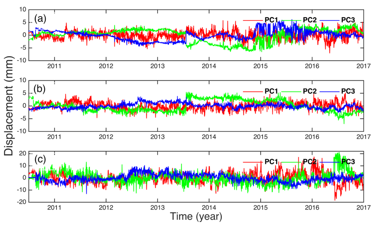
2.2. Common Mode Errors

The Global Navigation Satellite System (GNSS) provides an effective technique for monitoring the movement of the crust. Previous studies found that time series produced from CGPS arrays (after fitting and removing the linear trend) reveal significant seasonal variations [26,27,28,29,30]. The strong seasonal annual and semiannual signals identified at the majority of sites are believed to be driven by redistributions of temporal mass [27,31,32]. Dong et al. [27] showed that the coupled contributions from surface redistribution are the primary drivers of the observed seasonal oscillation of site positions; these mass loadings and pole tides can contribute about 66 % of the power of the observed seasonal signals. A large proportion of residual seasonal power is probably still induced by the effects of both unmodeled and mismodeled seasonal errors (i.e., common mode errors). These sources of error are the prominent residuals in GPS daily solutions: the inaccuracies in GPS measures consistently manifested as mixed time series seasonal variations, and different GPS stations presenting spatial correlation errors, which can likely be attributed to the uncorrected environmental effects of loading, satellite orbit biases, errors in the system, and other mismodeled residual faults, or a mixture of these GPS signals. These lead to biased interpretations of certain geophysical phenomena. These mismodeled effects in continuous GPS time series can be well described as colored noise [33,34]. The effective of the removal and destruction of CMEs plays a vital role in further enhancing the correctness of GPS data analysis [35].
Methods of filtering have been produced to eliminate CMEs from the GPS time series. Spatial filtering can effectively improve the accuracy of a coordinate time series for regional GPS networks by weakening CMEs, thereby supplying improved resolution for identifying transient or weak signals of deformation [36]. A spatial filtering method based on principal component analysis (PCA) was introduced by Dong et al. [27] to reduce the CMEs and offsets from the GPS residual time series. Here, we adopted the PCA technique to decompose time series into temporal principal components (PCs) and spatial eigenvectors, which are arranged according to the powers contributed by each PC. The regional temporal variation characteristics of the station network can be well illustrated by the contributions of the first several PCs, and the corresponding eigenvectors of these PCs also indicate the distribution in the space of the strength of the variations over time. In general, the signals impact the calculations of velocities using the GPS time series over the long term. Therefore, there is a requirement to employ only the lower-order PCs. Based on the results by other researchers, the first three PCs of our results were investigated to calculate the CME corrections [17,25,26,36,37]. Briefly, the processing steps are illustrated as follows:
Step 1: Quasi-Observation Combination Analysis (QOCA) software has been adopted to eliminate the CMEs within the time series of GPS measures [38]. The trend terms, seasonal signals of deformation from the raw GPS time series, and offsets have been removed to obtain GPS daily residual time series. Any postseismic and coseismic effects mixed in the raw GPS time series will be calculated as an offset and must be removed before applying spatial filtering [17,26]. Times series of the first three PCs are presented in Figure 3.
Step 2: The maximum likelihood estimation (MLE) method was applied to analyze the GPS uncertainties and velocities; the Create and Analyse Time Series (CATS, version, Manufacturer, Liverpool, UK) software was used to identify the velocities of all GPS stations. Research suggests that campaign-mode GPS stations could be described as white noise mode [25], and noise in the GPS time series is better described as a combination of white and flicker noises [26,33,39,40]. In this paper, a white noise model for campaign-mode GPS stations and a white noise plus flicker noise model for the continuous GPS stations were used to calculate velocities and associated representative uncertainties. As the ITRF 2014 is a non-rotating frame, to study the horizontal crustal movement of the NET, all the GPS horizontal velocities were converted to the Eurasian frame based on the rotating Euler pole transformation parameters [41]. Figure 4 shows the results of the uncertainties in velocity on the three components with unfiltered and filtered CMEs in the GPS time series presented in Figure 3; the horizontal velocity derived from the GPS time series is shown in Figure 5.

3. GRACE Data and Processing

Mass of non-tidal ocean redistribution, changes in global atmospheric surface pressure, and conversion of terrestrial water storage (snow, soil moisture, and groundwater) resulted in periodic and long-term deformation of the crust [42]. In this study, in order to match the GPS time series, the 2018 Grace Static Field Geopotential Coefficients CSR V 6.0 (RL06) product (University of Texas Center for Space Research) was applied from April 2002 to June 2017 to identify the oscillating signal of hydrological seasonal loading (Link to RL06 using the http://icgem.gfz-potsdam.de/series/10.5067/GRGSM-20C06, accessed on 20 September 2021). Like the RL05 GSM product, the RL06 GSM contains the contribution of hydrological variations, changes to the cryosphere, episodic processes, alterations to the background gravity models, and glacial isostatic adjustment (GIA). The new RL06 GRACE gravity field solutions applied improved parameters, processing algorithms, and data editing, and non-tidal variability in the atmosphere and ocean was removed by using the AOD1B Released-06 product [25,43]. With the new GRACE release 06 solution, the estimation quality and accuracy of mass redistribution have been significantly improved, and the noise in the GRACE gravity field solutions has been reduced considerably [44,45,46].
The geocenter motion corresponding to degree-1 Stokes coefficients was replaced [47] to increase the precision of spherical harmonic coefficients of low degree. Additionally, the C20 terms were substituted with the outputs of the satellite laser-ranging (SLR) experiments [48,49].
Then, equivalent water height (EWH) expresses the change in surface density (i.e., mass/area), retrieved from changes in the geoid coefficients [50]:
Δ σ θ , ϕ = a ρ e 3 ρ w l = 0 2 l + 1 1 + k l × m = 0 l Δ C l m cos m ϕ + Δ S l m sin m ϕ P ¯ l m cos θ
where ρ e represents the mean density of the entire earth and the ρ w is water density; a represents the average radius of the earth; Δ C l m and Δ S l m are changes in the monthly Stokes coefficients relating to the mean field; θ and ϕ are colatitude and longitude, respectively; k l   of degree l represents the loading Love number accounting for the elastic deformation of the earth under the particular mass load; and P ¯ l m represents the completely normalized Legendre functions, order m and degree l .
The non-tidal ocean and atmospheric loading were not removed from the GPS time series. Therefore, the AOD1B release 06 product GAC has been added to the GSM products to retain the vertical deformation consistency inferred from both GRACE and GPS measurements [43]. Then, the elastic displacement in height that is mainly caused by the surface mass load changes of hydrological, non-tidal, and atmospheric loading can be calculated using spherical harmonic coefficients of the gravity field and Love numbers [11,12,51]:
Δ h θ , ϕ = a l = 1 m = 0 l P ¯ l m cos θ Δ C l m cos m ϕ + Δ S l m sin m ϕ h l 1 + k l
where k l and h l are load Love numbers, respectively. A 300 km radius Gaussian smoothing and P4M6 (order m = 6 with a polynomial of degree 4) decorrelation filter have been applied to suppress the north-south stripe noise in the GRACE data [45,52].

4. Results and Discussion

4.1. Influence of CMEs on the Evaluation of GPS Velocities

At present, the mechanism of the geophysical response of nonlinear signals in CGPS time series has always been one of the focuses of GPS time series research; due to the regional differences in physical mechanism, it is difficult to model effectively. The mechanism of CMEs in the GPS time series is also one of the unsolved problems; studies have shown that the regional surface mass load may contribute to the CMEs present in the GPS time series, but this could not be satisfactorily explained [25,26]. Therefore, to obtain more reliable three-dimensional velocities, the residual CMEs were filtered out from the original GPS time series.
Following Dong et al. [36], the principal components and the spatial eigenvectors were applied to conduct the correction of GPS time series and the regional filtering [48]. Figure 3a–c shows the PC1–PC3 for east, north, and up components decomposed by PCA from regional GPS time series; their corresponding power spectral densities are normalized for comparison in Figure 6(a1,b1,c1). The average response of the spatial eigenvectors of PC1–PC3 for the east component were 75.87%, −14.35%, and 16.22%, respectively; for the north component, the figures were 79.22%, −13.21%, and −31.15%, respectively; for the up component, the figures were 90.95%, 14.68%, and −24.51%, respectively. This clearly indicates that PCA decomposition is based on a criterion of pattern power; PC contained the pattern with the highest power, and so on for subsequent PCs [53]. Therefore, we truncated the frequency band from 0 to 1.8 cpy of PC1, as shown in Figure 6(a2,b2,c2). The figures show that the power spectra of the CME time series obtained in the present study are consistent with the loading-induced time series; the seasonal signals are evident for the east, north, and up elements. A significant quasi-biennial oscillation (QBO) signal was detected in both the east and up elements, and the amplitude in the north component was nearly twice as much as that of the east component, which may be the quasi-periodic oscillation of the wind component in the lower stratosphere from the equatorial region [54]. Additionally, a quasi-8.5 year signal was detected in both the north and up components, which had been confirmed by Ding et al. [55,56] in the length of day variations (LOD), but the mechanism is still unclear. Results indicate that the effect of CMEs represents an additional driver of the seasonal variations in the GPS time series [26].
Figure 4 illustrates the impacts of CME filtering on the GPS velocity uncertainties; after the CMEs are filtered out, the signal-to-noise ratio of the GPS time series is considerably increased. The large discrepancies are noted for stations with short time durations, in which regional filtering advances the estimation of velocity due to the east component, at which short-term estimates of velocity can be biased by systematic errors [53], and sites with longer observation periods could get more high precision. After filtering out the CMEs, uncertainties in velocity ranged from 0.043 to 0.300 mm/yr, 0.038 to 0.248 mm/yr, and 0.111 to 0.910 mm/yr for the east, north, and up components, respectively, with a corresponding standard deviation of 0.045 mm/yr, 0.038 mm/yr, and 0.144 mm/yr, respectively. Differences in the uncertainty of velocities calculated from the unfiltered and filtered time series are significant differences; the vertical velocity uncertainly reduced by about 82.05%, while the east and north components improved by about 21.42% and 40.21%, respectively. The above results show that removing the CMEs using PCA analysis could more effectively and reliably suppress the signals of regional impact and achieve a significant improvement in the signal-to-noise ratio of the GPS time series. Therefore, they were chosen as the applications for the analysis of deformation and other GPS geophysical analyses.

4.2. Analysis of Surface Vertical Seasonal Loading

Figure 7 shows that substantial mass variations have been detected by GRACE, with clear negative mass loss signals in the southwestern area and positive mass increase signals in the middle area. Previous research suggests that the mass loss may attribute to deglaciation and snowmelt, while the mass increase may contribute to the significant lake level rise in the TP [57,58,59,60]. Kuang et al. (2016) indicated that observations in several previous studies from meteorological stations over the long term suggested that the TP’s temperature significantly increased over different periods since the 1950s, ranging from 0.16 to 0.67 °C decades−1. Meanwhile, there were increases in annual precipitation in most areas of the TP [57]. In particular, higher sensitivity to warming was exhibited by areas of higher elevation, showing accelerated glacier melting [58]. Jacob et al. [59] indicated that much of the high mountains of Asia is permafrost, and the limited capacity of the frozen ground would inhibit local recharge. Zhang et al. [60] used four to seven years of ICESat data and GRACE data in finding that the GRACE measurements of increased mass could be mainly attributed to the increased water level/mass in lakes. A major driver of this phenomenon is glacier melting; however, glacier melting should not increase the overall mass, as a fraction of meltwater would be evaporated or will flow downriver leaving the TP. In particular, precipitation in the TP over the last few decades shows a significant increase [60,61,62]. Additionally, a broad-scale tectonic uplift would be isostatically compensated by an increasing mass deficiency at depth, with attribute little effect attributed to gravity, as well as the impact of the ongoing viscoelastic response of the earth to past glacial unloading [59].
According to Equation (2), we obtained the long-term elastic vertical displacement mainly caused by redistribution of terrestrial water storage, as shown in Figure 7 of black arrows. All of the non-tectonic processes (e.g., alterations in the surface pressure of the global atmosphere, redistribution of the mass of the non-tidal ocean, and alteration of terrestrial water storage) and the deep tectonic processes can be attributed to the surface ground deformation; all of these signals could be well detected by GPS observations. As a result, the GPS time series may include incorrect signals. These signals may impact the precision of the estimated rates of vertical deformation of the crust. Therefore, the linear vertical rates derived from GRACE, resulting from the redistribution of mass, have been eliminated from actual GPS-derived vertical rates to constrain the tectonic deformation, as represented in Figure 8.

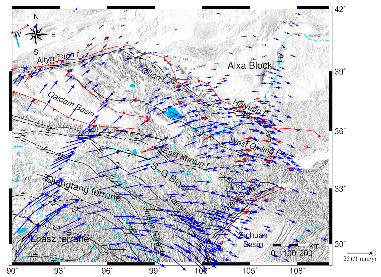
4.3. Three Dimensional Crustal Deformation Rates

Figure 5 shows the horizontal velocity derived from the GPS time series. All of the GPS horizontal velocities have been converted to the Eurasian frame based on the rotating Euler pole transformation parameters. The entire NET presents an overall clockwise rotation from north to south. The Qaidam Basin is moving northeastward about 8 mm/yr, and the horizontal velocities in the Northern Qilian mountains, between the main Qilian faults and the northern Qilian faults, are showing a significant decreasing trend, while the crustal shortening rates have increased significantly, indicating that the Northern Qilian area may experience strong compressive thrust nappe tectonic movements. The velocity field shows an east-west trend along the Altyn Tagh fault (i.e., the junction of the Northern margin NET and the Tarim Basin), which is in line with the strike-slip characteristic of the fault, and its strike-slip speed is about 5–10 mm/yr.
The NET is blocked by the northern Alxa and Orods Craton blocks, and the crust has been significantly shortened in the Qilian Mountains and the Longmen Mountains, with a horizontal convergence rate reaching about 10 mm/yr. The horizontal movement from the east of the Qaidam Basin to the northeastern margin of the Liupan Shan area is complex; the movement direction on the west side is NE; in the central part, it changed to an approximate EW direction; then, it gradually changed to an ES direction to the east. The movement has sinistral shearing in the entire Qilian Mountains due to the eastward escaping of the NET, which is a strong earthquake belt in the NET. This reveals that the tectonic activities are distributed throughout the whole Qilian mountains. Horizontal velocities are relatively consistent: in the south of the Haiyuan fault, the horizontal velocity approximately 8–10 mm/yr, while it is approximately 5 mm/yr in the north of the Haiyuan fault.
Blocked by the Yangtze block, the crust was significantly shortened in the Longmen Shan area. With the Longmen Shan and Xiaojiang faults as the boundary, the crust moved southeastward at a speed of 5–10 mm/yr. Compared with the velocity vector of movement on the eastern margin of the TP, it can be seen that the Yangtze block craton, as a rigid block blocking the eastward movement of the plateau, is the key to the uplift of the plateau and the material migration pattern in the Sichuan-Yunnan region.
Figure 8 shows the corrected vertical velocity field, highlighting the complex vertical crustal deformation. In this study, 39 continuous GPS time series and GRACE data have been applied with improved processing strategies to constrain the vertical tectonic deformations of the entire NET and its surroundings. This reveals the current vertical movement characteristics of the NET. From the boundary effect of the impact between the Eurasian and Indian plates to the slow crustal uplift caused by the compression inside the plateau, several movement patterns have been formed in the eastern marginal area, such as crustal compression and internal block thrusting.
The vertical crustal deformation fields have been calculated to help explain their dynamics process in our experiment. The results indicate that the whole NET is mainly uplifting after eliminating the elastic deformation effects from the GPS velocities. Rates of crustal uplift of about 1–4 mm/yr in the Qaidam Basin and the Qilian Mountains. Inland basins have played a vital role in the growth of the TP, such as the Tarim Basin, the Qaidam Basin, and the Sichuan Basin. Under the current geological structure, a basin will continue to show a downward trend due to the compression of the surrounding mountains (e.g., the Tarim Basin and the Qaidam Basin both express a different degree of crust subsidence). Figure 8 shows that two GPS stations are subsiding at the junction of the northern margin of the Altyn Tagh fault and the Qadim Basin, revealing the dynamic process of the Tarim Basin’s thrusting into the TP after the internal collision.
The southeastern part of the TP is an essential channel for materials to escape eastward, which adjusts the mass change of the entire TP. As the Sichuan Basin is located in the Yangtze block, its primary function is to block the eastward movement of the TP, leading to the north-south diversion of crustal materials. By thrusting beneath the Longmen Shan, the Sichuan Basin plays a vital role in the evolution and growth of the Longmen Shan faults. As a result, under the strong compression and thrust between eastern Tibet and the surrounding rigid blocks, the unusual crustal uplift rates reached about 7.13 ± 0.53 mm/yr in the Longmen Shan fault.

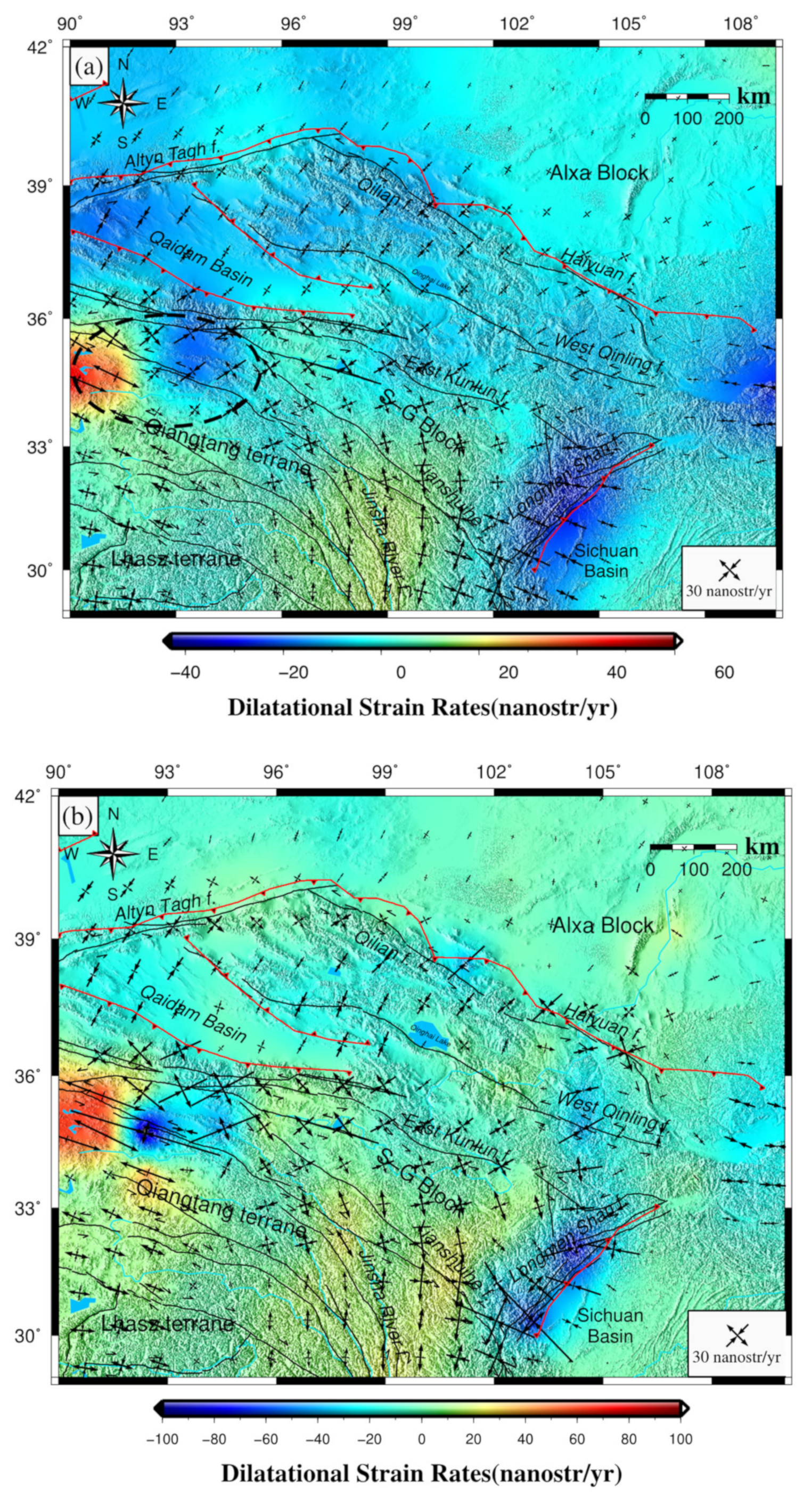
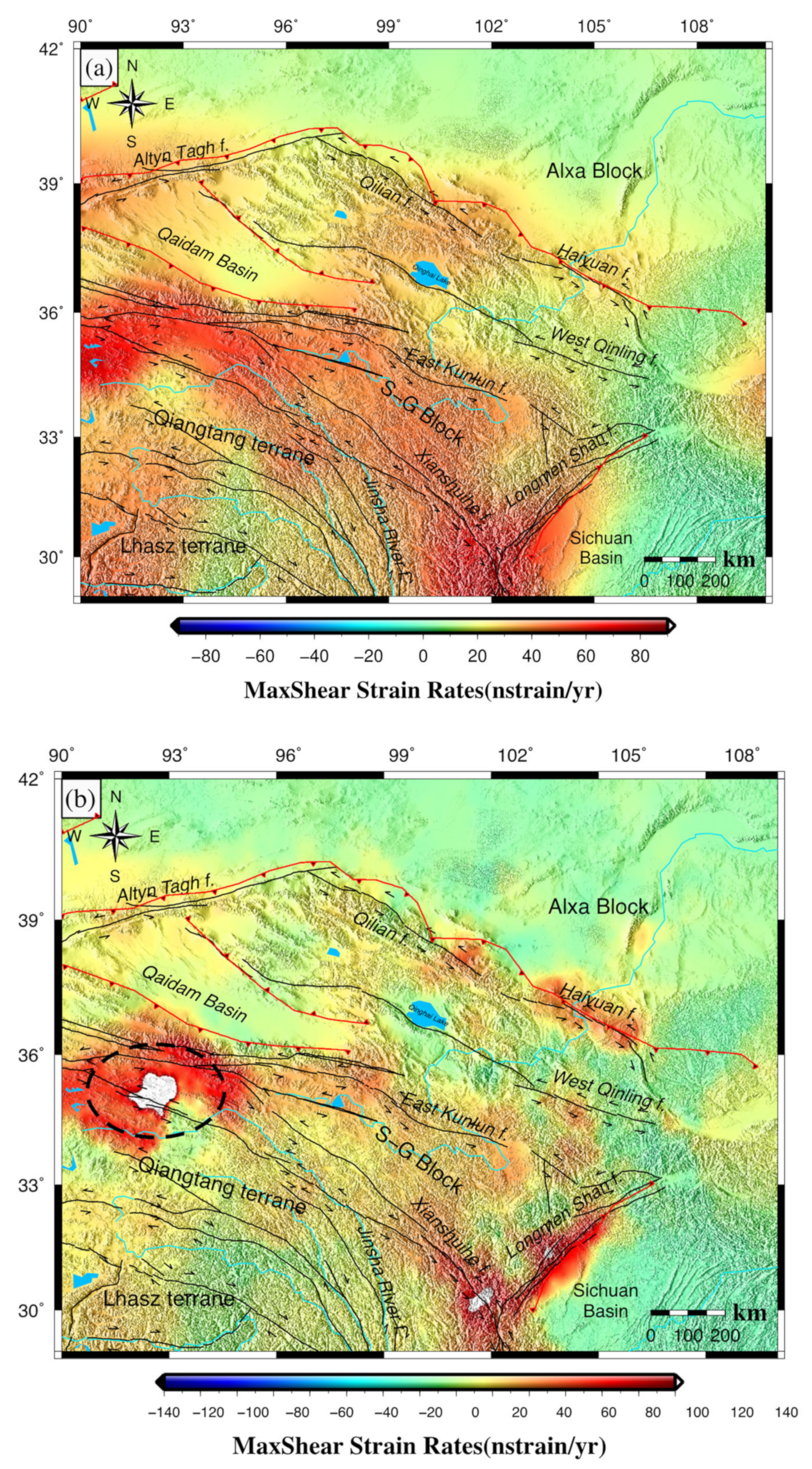
4.4. Dilatation Strain and Maximum Shear Strain Rates of the Plateau

The continental impact between the Eurasian and Indian plates has driven crustal shortening of the Tibetan Plates and their surroundings, and this shortening is mainly absorbed by the crustal thickening and strike-slip of the TP. Consequently, tectonic movement is the most direct dynamic manifestation of continental collision. As the surface displacement is only the change in the spatial geometric quantity, the strain that causes displacement always needs to be considered. Therefore, estimating the 2D strain field based on GPS observations of horizontal velocities is crucially essential in explaining the dynamic mechanism of the TP. The strain field of the crust could reflect the regional tectonic characteristics, and at the same time could be used to reveal the regional tectonic dynamics process and provide valuable parameters for the study of fault strain accumulation, crustal uplift or subsidence, and seismic risk assessment.
The main theory for calculating 2D principal strain, maximum shear strain, and dilatational strain is shown by the following equations:
Δ U E Δ U N = U E E U E N U N E U N N Δ E Δ N = U E E 1 2 U E N + U N E 1 2 U N E + U E N U N N + U E E 1 2 U E N U N E 1 2 U N E U E N U N N = ε Δ P + d R Δ P  
where Δ U = Δ U E , Δ U N T is horizontal displacement between two points, Δ P = ( Δ E , Δ N ) T is the difference of latitude and longitude, and ε and d R are strain tensor and rotation tensors. The maximum and minimum principal strains are:
ε 1 = ε e + ε n 2 + 1 2 ε e ε n 2 + 2 ε e n 2 ε 2 = ε e + ε n 2 1 2 ε e ε n 2 + 2 ε e n 2  
maximum shear strain:
γ m a x = ε 1 ε 2 = ε e ε n 2 + 2 ε e n 2
dilatational strain:
Δ = ε 1 + ε 2 = ε e + ε n
In this study, the SSPX software was applied to determine the 2D strain field (available at http://homepage.mac.com/nfcd/work/programs.html, accessed on 10 April 2022), following the processing strategies provided by Cardozo and Allmendinger [63]. The grid-distance weighted routine with α = 100 km and the grid-nearest neighbor routine with 12 neighbors and a maximum radius = 300 km were applied to obtain the dilatational rates of strain, as shown in Figure 9a,b, as well as in Figure 10. We found that the grid-nearest neighbor routine has better spatial characteristics than the grid-distance weighted routine, which might be due to distance smoothing.
The results suggest that horizontal compressive strain and dilatation are distributed throughout the whole plateau. In particular, Figure 9a shows that dilatation in the Altyn Tagh fault, the northern part of the Qaidam Basin, the middle area of the Qilian Mountains, the East Kunlun fault, the West Qinling fault, and the Longmen Shan fault are mainly negative, which coincides with the distribution of earthquakes illustrated in Figure 1. Generally, earthquakes are products of long-term strain accumulation and energy release in crustal movement; they always occur in areas with significant movement differences (i.e., areas with various tectonic rates and directions). Previous studies also suggested that areas with compression may be a response to the strain accumulation, while areas with extension may be a response to the magnitude of earthquakes [8]. Combining the corrected vertical crustal velocity with the dilatational strain field from the horizontal velocity, we conclude that Northeastern Tibetan is suffering from crustal shortening and thickening. Meanwhile, the compression strain is significant under the strong interaction between eastern Tibetan and the surrounding rigid blocks, corresponding to the unusual crustal uplift rates.
Figure 10 shows that areas with high maximum shear strain rates are mainly distributed in the Altyn Tagh fault, the Qilian Shan faults, the Haiyuan fault, the West Qinling fault, the East Kunlun fault, and the Longmen Shan fault; these areas also coincide with the distribution of earthquakes as illustrated in Figure 1. Notably, there have abnormal maximum shear strain rate values in the west of the East Kunlun fault (e.g., the area with the blue-dashed ellipse in Figure 10b); this may be due to the lack of GPS observations that are able to illustrate satisfactorily the strain characteristics of this area [8]. This could also explain the abnormal dilatation, which is circled by a red-dashed ellipse, as shown in Figure 9a. Additionally, the northern margin of the TP shows sinistral strike-slip movement in the Altyn Tagh fault, the Qilian Shan faults, the Haiyuan fault, and the West Qinling fault. In the eastern TP, which is blocked by the rigid Sichuan block and bounded by the Longmen Shan fault, the crustal has been divided mainly into two channels. One is extruded along the Xianshui He and Xiaojiang fault in the EEN direction, which results in good mutual authenticating with the dilatation, and the other way is extruded along the Longmen Shan fault in the EN direction.

5. Conclusions

We used 39 continuous and 451 campaign-mode GPS stations of the CMONOC to estimate the 3D crustal deformation velocities and strain field features in and around NET. Comparing the difference in velocities with unfiltered and filtered CMEs confirmed that the vertical rate uncertainty had reduced by about 82.05%, while the east and north components have improved by approximately 21.42% and 40.21%, respectively. This could suppress the regional effect signals more effectively and reliabily and obtain a significant gain in the GPS time series signal-to-noise ratio.
The contemporary 3D velocity was presented to interpret the plateau’s crustal deformation and dynamic processes. The results suggest that the entire NET shows an overall clockwise movement from EN to ES and is bounded by the Qilian and Haiyuan faults; the relative compression from NE to NEE between the blocks on both sides is evident. Corrected vertical crustal deformation results indicate that both the crustal uplift and the subsidence are anisotropic in NET, and that the maximum uplift rate in the Longmen Shan fault reaches 7.13 ± 0.53 mm/yr. According to the correct velocities and the horizontal strain fields of the NET, this revealed that the crustal vertical uplift and subsidence are closely related to the characteristics of the strain field. Due to the subduction and compression of the inland, the entire crust is uplifting in the margin, indicating that the shortening of the crust is the main driver of the uplift of the TP. A combined analysis of the shortening of the crust and the maximum shear strain pattern allowed an understanding of the tectonic processes within the NET.
It should be noted that there was an abnormal rate of strain values in the areas that were lacking GPS observations, and that we are unable to illustrate the strain characteristics of this area well. Therefore, it is necessary to adopt more observation methods (e.g., we are currently using the InSAR method) to obtain higher-precision and higher-resolution 3D crustal movements and strain fields in further research.

Author Contributions

Conceptualization, T.Z. and L.H.; methodology, T.Z.; software, T.Z.; validation, Z.S. and W.L.; writing—original draft preparation, T.Z.; writing—review and editing, L.H. and Z.S.; supervision, W.S. All authors have read and agreed to the published version of the manuscript.

Funding

This research was funded by the National Natural Science Foundation of China (NSFC) (Grant Nos. 42030105, 41804012, 42104023, 42004006), the Natural Science Foundation of Hubei Province (Grant No. 2019CFB611), the Education Commission of Hubei Province of China (Grant No. Q20212801), the Space Station Project (2020)228, the PhD Research Start-up Foundation of Hubei University of Science and Technology (Grant Nos. L07903/170468, L07903/170469), and the Open Research Fund Program of the Key Laboratory of Geospace Environment and Geodesy, Ministry of Education, China (Grant No. 20-01-03). Support was also received from the Key Laboratory of Geography and National Condition Monitoring, the Ministry of Natural Resources (2022NGCM01), the Natural Science Foundation of Gansu Province (20JR10RA271), “Tianyou Youth Talents Supporting Project” Program of Lanzhou Jiaotong University (Li Wei) and China Postdoctoral Science Foundation (2019M660091XB).

Data Availability Statement

The data that used in this study can be requested by contacting the first author.

Acknowledgments

The authors gratefully appreciate the “Crustal Movement Observation Network of China” for providing the GPS data and JPL for providing the GIPSY/OASIS-II software. We also thank NASA via the Center of Space Research (CSR) for providing the monthly gravity field products. Some of the figures were plotted using the Generic Mapping Tools (GMT) software, developed by Wessel and Smith (1991).

Conflicts of Interest

The authors declare no conflict of interest.

References

  1. Yin, A.; Harrison, T.M. Geologic Evolution of the Himalayan-Tibetan Orogen. Ann. Rev. Earth Planet. 2003, 28, 211–280. [Google Scholar] [CrossRef] [Green Version]
  2. Molnar, P.; England, P.; Martinod, J. Mantle Dynamics, Uplift of the Tibetan Plateau, and the Indian Monsoon. Rev. Geophys. 1993, 31, 357–396. [Google Scholar] [CrossRef]
  3. Tapponnier, P. Oblique Stepwise Rise and Growth of the Tibet Plateau. Science 2001, 294, 1671–1677. [Google Scholar] [CrossRef]
  4. Zhao, Q.; Wu, W.; Wu, Y. Using Combined GRACE and GPS Data to Investigate the Vertical Crustal Deformation at the Northeastern Margin of the Tibetan Plateau. J. Asian Earth Sci. 2017, 134, 122–129. [Google Scholar] [CrossRef]
  5. Zhou, M.D.; Zhang, Y.S.; Shi, Y.L.; Zhang, S.X.; Fan, B. Three-Dimensional Crustal Velocity Structure in the Northeastern Margin of the Qinghai-Tibetan Plateau. Prog. Geophys. 2006, 21, 127–134. [Google Scholar]
  6. Shen, Z.K.; Lü, J.; Wang, M.; Bürgmann, R. Contemporary Crustal Deformation around the Southeast Borderland of the Tibetan Plateau. J. Geophys. Res. Solid Earth 2005, 110. [Google Scholar] [CrossRef] [Green Version]
  7. Wang, Q. Present-Day Crustal Deformation in China Constrained by Global Positioning System Measurements. Science 2001, 294, 574–577. [Google Scholar] [CrossRef] [PubMed] [Green Version]
  8. Qu, W.; Gao, Y.; Chen, H.; Liang, S.; Han, Y.; Zhang, Q.; Wang, Q.; Hao, M. Review on Characteristics of Present Crustal Tectonic Movement and Deformation in Qing- Hai-Tibet Plateau, China Using GPS High Precision Monitoring Data. J. Earth Sci. Environ. 2021, 43, 182–204. [Google Scholar]
  9. Wang, M.; Shen, Z. Present-Day Crustal Deformation of Continental China Derived From GPS and Its Tectonic Implications. J. Geophys. Res. Solid Earth 2020, 125, e2019JB018774. [Google Scholar] [CrossRef] [Green Version]
  10. Wu, Y.; Zheng, Z.; Nie, J.; Chang, L.; Su, G.; Yin, H.; Liang, H.; Pang, Y.; Chen, C.; Jiang, Z.; et al. High-Precision Vertical Movement and Three-Dimensional Deformation Pattern of the Tibetan Plateau. J. Geophys. Res. Solid Earth 2022, 127, e2021JB023202. Available online: https://agupubs.onlinelibrary.wiley.com/doi/epdf/10.1029/2021JB023202 (accessed on 10 April 2022). [CrossRef]
  11. van Dam, T.; Wahr, J.; Lavallée, D. A Comparison of Annual Vertical Crustal Displacements from GPS and Gravity Recovery and Climate Experiment (GRACE) over Europe. J. Geophys. Res. 2007, 112. [Google Scholar] [CrossRef] [Green Version]
  12. Fu, Y.; Freymueller, J.T. Seasonal and Long-Term Vertical Deformation in the Nepal Himalaya Constrained by GPS and GRACE Measurements. J. Geophys. Res. Solid Earth 2012, 117. [Google Scholar] [CrossRef]
  13. Hao, M.; Freymueller, J.T.; Wang, Q.; Cui, D.; Qin, S. Vertical Crustal Movement around the Southeastern Tibetan Plateau Constrained by GPS and GRACE Data. Earth Planet. Sci. Lett. 2016, 437, 1–8. [Google Scholar] [CrossRef]
  14. Pan, Y.; Shen, W.-B.; Shum, C.K.; Chen, R. Spatially Varying Surface Seasonal Oscillations and 3-D Crustal Deformation of the Tibetan Plateau Derived from GPS and GRACE Data. Earth Planet. Sci. Lett. 2018, 502, 12–22. [Google Scholar] [CrossRef]
  15. Liang, S.; Gan, W.; Shen, C.; Xiao, G.; Liu, J.; Chen, W.; Ding, X.; Zhou, D. Three-dimensional Velocity Field of Present-day Crustal Motion of the Tibetan Plateau Derived from GPS Measurements. J. Geophys. Res. Solid Earth 2013, 118, 5722–5732. [Google Scholar] [CrossRef]
  16. Zumberge, J.F.; Heflin, M.B.; Jefferson, D.C.; Watkins, M.M.; Webb, F.H. Precise Point Positioning for the Efficient and Robust Analysis of GPS Data from Large Networks. J. Geophys. Res. 1997, 102, 5005–5017. [Google Scholar] [CrossRef] [Green Version]
  17. Zhang, T.; Shen, W.B.; Pan, Y.; Wei, L. Study of Seasonal and Long-Term Vertical Deformation in Nepal Based on GPS and GRACE Observations. Adv. Space Res. 2018, 61, 1005–1016. [Google Scholar] [CrossRef]
  18. Schmid, R.; Dach, R.; Collilieux, X.; Jäggi, A.; Schmitz, M.; Dilssner, F. Absolute IGS Antenna Phase Center Model Igs08.Atx: Status and Potential Improvements. J. Geod. 2016, 90, 343–364. [Google Scholar] [CrossRef] [Green Version]
  19. Petit, G.; Luzum, B. (Eds.) IERS Conventions (2010); IERS Technical Note; No. 36; Verlag des Bundesamts für Kartographie und Geodäsie: Frankfurt am Main, Germany, 2010. [Google Scholar]
  20. Boehm, J.; Heinkelmann, R.; Schuh, H. Short Note: A Global Model of Pressure and Temperature for Geodetic Applications. J. Geod. 2007, 81, 679–683. [Google Scholar] [CrossRef]
  21. Zhang, K.L.; Liang, S.M.; Gan, W.J. Crustal Strain Rates of Southeastern Tibetan Plateau Derived from GPS Measurements and Implications to Lithospheric Deformation of the Shan-Thai Terrane. Earth Planet. Phys. 2019, 3, 47–54. [Google Scholar] [CrossRef]
  22. Farrell, W.E. Deformation of the Earth by Surface Loads. Rev. Geophys. 1972, 10, 761–797. [Google Scholar] [CrossRef]
  23. Zheng, G.; Wang, H.; Wright, T.J.; Lou, Y.; Zhang, R.; Zhang, W.; Shi, C.; Huang, J.; Wei, N. Crustal Deformation in the India-Eurasia Collision Zone From 25 Years of GPS Measurements: Crustal Deformation in Asia From GPS. J. Geophys. Res. Solid Earth 2017, 122, 9290–9312. [Google Scholar] [CrossRef]
  24. Altamimi, Z.; Rebischung, P.; Métivier, L.; Collilieux, X. ITRF2014: A New Release of the International Terrestrial Reference Frame Modeling Nonlinear Station Motions. J. Geophys. Res. Solid Earth 2016, 121, 6109–6131. [Google Scholar] [CrossRef] [Green Version]
  25. Pan, Y.; Chen, R.; Ding, H.; Xu, X.; Zheng, G.; Shen, W.; Xiao, Y.; Li, S. Common Mode Component and Its Potential Effect on GPS-Inferred Three-Dimensional Crustal Deformations in the Eastern Tibetan Plateau. Remote Sens. 2019, 11, 1975. [Google Scholar] [CrossRef] [Green Version]
  26. He, X.; Hua, X.; Yu, K.; Xuan, W.; Lu, T.; Zhang, W.; Chen, X. Accuracy Enhancement of GPS Time Series Using Principal Component Analysis and Block Spatial Filtering. Adv. Space Res. 2015, 55, 1316–1327. [Google Scholar] [CrossRef]
  27. Dong, D.; Fang, P.; Bock, Y.; Cheng, M.K.; Miyazaki, S. Anatomy of Apparent Seasonal Variations from GPS-Derived Site Position Time Series. J. Geophys. Res. B Solid Earth 2002, 107, ETG 9-1–ETG 9-16. [Google Scholar] [CrossRef] [Green Version]
  28. Ray, J.; Altamimi, Z.; Collilieux, X.; Van Dam, T. Anomalous Harmonics in the Spectra of GPS Position Estimates. GPS Solut. 2008, 12, 55–64. [Google Scholar] [CrossRef]
  29. Van Dam, T.; Collilieux, X.; Wuite, J.; Altamimi, Z.; Ray, J. Nontidal Ocean Loading: Amplitudes and Potential Effects in GPS Height Time Series. J. Geod. 2012, 86, 1043–1057. [Google Scholar] [CrossRef] [Green Version]
  30. Jiang, W.-P.; Deng, L.; Li, Z.; Zhou, X.; Liu, H. Effects on Noise Properties of GPS Time Series Caused by Higher-Order Ionospheric Corrections. Adv. Space Res. 2014, 53, 1035–1046. [Google Scholar] [CrossRef]
  31. Blewitt, G.; Lavallee, D.; Clarke, P.; Nurutdinov, K. A New Global Mode of Earth Deformation: Seasonal Cycle Detected. Science 2001, 294, 2342–2345. [Google Scholar] [CrossRef] [Green Version]
  32. Jiang, W.-P.; Li, Z.; Van Dam, T.; Ding, W. Comparative Analysis of Different Environmental Loading Methods and Their Impacts on the GPS Height Time Series. J. Geod. 2013, 87, 687–703. [Google Scholar] [CrossRef]
  33. Williams, S.; Bock, Y.; Fang, P.; Jamason, P.; Nikolaidis, R.M.; Prawirodirdjo, L.; Miller, M.; Johnson, D.J. Error Analysis of Continuous GPS Time Series. J. Geophys. Res. Solid Earth 2004, 109. preprint. [Google Scholar] [CrossRef] [Green Version]
  34. Amiri-Simkooei, A.; Tiberius, C.C.J.M.; Teunissen, P. Assessment of Noise in GPS Coordinate Time Series: Methodology and Results. J. Geophys. Res. 2007, 112. [Google Scholar] [CrossRef] [Green Version]
  35. Bian, Y.; Yue, J.; Ferreira, V.G.; Cong, K.; Cai, D. Common Mode Component and Its Potential Effect on GPS-Inferred Crustal Deformations in Greenland. Pure Appl. Geophys. 2021, 178, 1805–1823. [Google Scholar] [CrossRef]
  36. Dong, D.; Fang, P.; Bock, Y.; Webb, F.; Prawirodirdjo, L.; Kedar, S.; Jamason, P. Spatiotemporal Filtering Using Principal Component Analysis and Karhunen-Loeve Expansion Approaches for Regional GPS Network Analysis: SPATIOTEMPORAL FILTERING GPS NETWORK. J. Geophys. Res. 2006, 111, B03405. [Google Scholar] [CrossRef] [Green Version]
  37. Ming, F.; Yang, Y.; Zeng, A.; Zhao, B. Spatiotemporal Filtering for Regional GPS Network in China Using Independent Component Analysis. J. Geod. 2017, 91, 419–440. [Google Scholar] [CrossRef]
  38. Dong, D.; Herring, T.A.; King, R.W. Estimating Regional Deformation from a Combination of Space and Terrestrial Geodetic Data. J. Geod. 1998, 72, 200–214. [Google Scholar] [CrossRef]
  39. Mao, A.; Harrison, C.; Dixon, T. Noise in GPS Coordinate Time Series. J. Geophys. Res. 1999, 104, 2797–2816. [Google Scholar] [CrossRef] [Green Version]
  40. Zhang, J.; Bock, Y.; Johnson, H.; Fang, P.; Williams, S.; Genrich, J.; Wdowinski, S.; Behr, J. Southern California Permanent GPS Geodetic Array: Error Analysis of Daily Position Estimates and Site Velocities. J. Geophys. Res. Solid Earth 1997, 102, 18035–18055. [Google Scholar] [CrossRef]
  41. Altamimi, Z.; Collilieux, X.; Métivier, L. ITRF2008: An Improved Solution of the International Terrestrial Reference Frame. J. Geod. 2011, 85, 457–473. [Google Scholar] [CrossRef] [Green Version]
  42. Tapley, B.D.; Bettadpur, S.; Ries, J.C.; Thompson, P.F.; Watkins, M.M. GRACE Measurements of Mass Variability in the Earth System. Science 2004, 305, 503–505. [Google Scholar] [CrossRef] [Green Version]
  43. University of Texas Center For Space Research (UTCSR). Grace Static Field Geopotential Coefficients CSR Release 6.0; UTCSR: Austin, TX, USA, 2018. [Google Scholar] [CrossRef]
  44. Dobslaw, H.; Bergmann-Wolf, I.; Dill, R.; Poropat, L.; Thomas, M.; Dahle, C.; Esselborn, S.; Knig, R.; Flechtner, F. A New High-Resolution Model of Non-Tidal Atmosphere and Ocean Mass Variability for de-Aliasing of Satellite Gravity Observations: AOD1B RL06. Geophys. J. Int. 2017, 221, 169–263. [Google Scholar] [CrossRef] [Green Version]
  45. Save, H.; Tapley, B.; Bettadpur, S. GRACE RL06 Reprocessing and Results from CSR; EGU General Assembly: Vienna, Austria, 2018. [Google Scholar]
  46. Göttl, F.; Schmidt, M.; Seitz, F. Mass-Related Excitation of Polar Motion: An Assessment of the New RL06 GRACE Gravity Field Models. Earth Planets Space 2018, 70, 195. [Google Scholar] [CrossRef]
  47. Swenson, S.C.; Chambers, D.P.; Wahr, J. Estimating Geocenter Variations from a Combination of GRACE and Ocean Model Output. J. Geophys. Res. Solid Earth 2008, 113(B8). [Google Scholar] [CrossRef] [Green Version]
  48. Cheng, M.; Tapley, B.D. Variations in the Earth’s Oblateness during the Past 28 Years. J. Geophys. Res. Solid Earth 2005, 109. [Google Scholar] [CrossRef]
  49. Cheng, M.; Tapley, B.D.; Ries, J.C. Deceleration in the Earth’s Oblateness. J. Geophys. Res. Solid Earth 2013, 118, 740–747. [Google Scholar] [CrossRef]
  50. Wahr, J.; Molenaar, M.; Bryan, F. Time Variability of the Earth’s Gravity Field: Hydrological and Oceanic Effects and Their Possible Detection Using GRACE. J. Geophys. Res. Solid Earth 1998, 103, 30205–30229. [Google Scholar] [CrossRef]
  51. Kusche, J.; Schrama, E. Surface Mass Redistribution Inversion from Global GPS Deformation and Gravity Recovery and Climate Experiment (GRACE) Gravity Data. J. Geophys. Res. Solid Earth 2005, 110, B09409. [Google Scholar] [CrossRef] [Green Version]
  52. Chen, J.L.; Wilson, C.R.; Li, J.; Zhang, Z. Reducing Leakage Error in GRACE-Observed Long-Term Ice Mass Change: A Case Study in West Antarctica. J. Geod. 2015, 89, 925–940. [Google Scholar] [CrossRef]
  53. Serpelloni, E.; Faccenna, C.; Spada, G.; Dong, D.; Williams, S.D.P. Vertical GPS Ground Motion Rates in the Euro-Mediterranean Region: New Evidence of Velocity Gradients at Different Spatial Scales along the Nubia-Eurasia Plate Boundary. J. Geophys. Res. Solid Earth 2013, 118, 6003–6024. [Google Scholar] [CrossRef] [Green Version]
  54. Belmont, A.D.; Dartt, D.G. Variation with Longitude of the Quasi-Biennial Oscillation. Mon. Weather Rev. 1968, 96, 767–777. [Google Scholar] [CrossRef] [Green Version]
  55. Ding, H. Attenuation and Excitation of the ∼6 Year Oscillation in the Length-of-Day Variation. Earth Planet. Sci. Lett. 2019, 507, 131–139. [Google Scholar] [CrossRef]
  56. Ding, H.; Jin, T.; Li, J.; Jiang, W. The Contribution of a Newly Unraveled 64 Years Common Oscillation on the Estimate of Present-Day Global Mean Sea Level Rise. J. Geophys. Res. Solid Earth 2021, 126, e2021JB022147. [Google Scholar] [CrossRef]
  57. Kuang, X.; Jiao, J.J. Review on Climate Change on the Tibetan Plateau during the Last Half Century. J. Geophys. Res. Atmos. 2016, 121, 3979–4007. [Google Scholar] [CrossRef]
  58. Guo, D.; Yu, E.; Wang, H. Will the Tibetan Plateau Warming Depend on Elevation in the Future? J. Geophys. Res. Atmos. 2016, 121, 3969–3978. [Google Scholar] [CrossRef] [Green Version]
  59. Jacob, T.; Wahr, J.; Pfeffer, W.T.; Swenson, S. Recent Contributions of Glaciers and Ice Caps to Sea Level Rise. Nature 2012, 482, 514–518. [Google Scholar] [CrossRef]
  60. Zhang, G.; Yao, T.; Xie, H.; Kang, S.; Lei, Y. Increased Mass over the Tibetan Plateau: From Lakes or Glaciers? Geophys. Res. Lett. 2013, 40, 2125–2130. [Google Scholar] [CrossRef]
  61. Zhang, G.; Xie, H.; Kang, S.; Yi, D.; Ackley, S.F. Monitoring Lake Level Changes on the Tibetan Plateau Using ICESat Altimetry Data (2003–2009). Remote Sens. Environ. 2011, 115, 1733–1742. [Google Scholar] [CrossRef]
  62. Xu, Z.X.; Gong, T.L.; Li, J.Y. Decadal Trend of Climate in the Tibetan Plateau-Regional Temperature and Precipitation. Hydrol. Process. 2010, 22, 3056–3065. [Google Scholar] [CrossRef]
  63. Cardozo, N.; Allmendinger, R.W. SSPX: A Program to Compute Strain from Displacement/Velocity Data. Comput. Geosci. 2009, 35, 1343–1357. [Google Scholar] [CrossRef]
Figure 1. Tectonic background in NET. The earthquake focal mechanisms are from the Global CMT (Centroid Moment Tensor) catalogue from 1 January 1976 to 1 January 2017. Main faults are annotated as black curves, and subduction zones are annotated as red curves.
Remotesensing 14 02638 g001
Figure 2. GPS site locations in northeastern Tibet, with 39 continuous stations and 451 campaign-mode stations. The red stars denote the continuous stations, and the green triangles denote the campaign-mode stations, with records spanning from March 2009 to January 2017.
Remotesensing 14 02638 g002
Figure 3. Time series of the first three principal components decomposed by PCA from regional GPS time series. (ac) denote the east, north, and up directions, respectively.
Remotesensing 14 02638 g003
Figure 4. The velocity uncertainly of the GPS time series in three different directions, east, north, and up, over NET. Blue and red circles represent the GPS time series unfiltered CMEs and filtered GPS time series, respectively.
Remotesensing 14 02638 g004
Figure 5. GPS-derived horizontal velocity field relative to stable Eurasia in NET; blue arrows and red arrows represent the velocities for campaign-mode stations and CGPS, respectively; the light gray ellipse at each velocity vector is 95% confidence.
Remotesensing 14 02638 g005
Figure 6. Normalized power spectra density of the first three principal components. (a1,b1,c1) denote the east, north, and up directions, respectively. (a2,b2,c2) denote the corresponding amplitude spectra of pc1, and the frequency ranges from 0 to 1.8 cycles per year (cpy).
Remotesensing 14 02638 g006
Figure 7. The CSR RL06 GRACE-derived mass change in terms of the secular trend of gravity change (colored background) from April 2002 to June 2017; black arrows denote elastic displacement in height, mainly caused by the surface mass redistribution, and thin black vertical lines are the rms. Glaciers on the Tibetan Plateau are marked as white dots, and lakes are marked as light blue patches.
Remotesensing 14 02638 g007
Figure 8. The CGPS-derived vertical velocity field relative to ITRF 2014 in NET Tibet; the blue vectors denote uplift, and the red vectors denote subsidence; the thin black vertical lines are the rms.
Remotesensing 14 02638 g008
Figure 9. GPS-derived rates of principal strain (arrow pairs) and dilatational rate of strain as continuous background color patterns using (a) the grid-distance weighted routine with α = 100 km, and (b) the grid-nearest neighbor routine with 12 neighbors and a maximum radius = 300 km, respectively. The color bars are different in each sub-figure to identify regional strain patterns. The red-dashed ellipse in sub-figure (a) represents the area with abnormal dilatational values.
Remotesensing 14 02638 g009
Figure 10. GPS-derived rates of maximum shear strain as a continuous background color pattern using (a) the grid-distance weighted routine with α = 100 km, and (b) the grid-nearest neighbor routine with 12 neighbors and a maximum radius = 300 km, respectively. The color bars are different in each sub-figure for the identification of regional strain patterns. The blue-dashed ellipse in sub-figure (b) represents the area with abnormal rates of maximum shear strain values.
Remotesensing 14 02638 g010
Publisher’s Note: MDPI stays neutral with regard to jurisdictional claims in published maps and institutional affiliations.

