Technical Note

An Improved Multi-Baseline Phase Unwrapping Method for GB-InSAR

1
Radar Research Lab, School of Information and Electronics, Beijing Institute of Technology, Beijing 100081, China
2
Key Laboratory of Electronic and Information Technology in Satellite Navigation (Beijing Institute of Technology), Ministry of Education, Beijing 100081, China
3
Beijing Institute of Technology Chongqing Innovation Center, Chongqing 401120, China
4
Advanced Technology Research Institute, Beijing Institute of Technology, Jinan 250300, China
*
Author to whom correspondence should be addressed.
Remote Sens. 2022, 14(11), 2543; https://doi.org/10.3390/rs14112543
Submission received: 19 April 2022 / Revised: 17 May 2022 / Accepted: 24 May 2022 / Published: 26 May 2022
(This article belongs to the Special Issue Advances in Synthetic Aperture Radar Remote Sensing)

Abstract

:
Ground-based interferometric synthetic aperture radar (GB-InSAR) technology can be applied to generate a digital elevation model (DEM) with high spatial resolution and high accuracy. Phase unwrapping is a critical procedure, and unwrapping errors cannot be effectively avoided in the interferometric measurements of terrains with discontinuous heights. In this paper, an improved multi-baseline phase unwrapping (MB PU) method for GB-InSAR is proposed. This method combines the advantages of the cluster-analysis-based MB PU algorithm and the minimum cost flow (MCF) method. A cluster-analysis-based MB PU algorithm (CA-based MB PU) is firstly utilized to unwrap the clustered pixels with high phase quality. Under the topological constraints of a triangulation network, the connectivity graph of any non-clustered pixel is established with its adjacent unwrapped cluster pixels. Then, the absolute phase of these non-clustered pixels can be identified using the MCF method. Additionally, a spatial-distribution-based denoising algorithm is utilized to denoise the data in order to further improve the accuracy of the phase unwrapping. The DEM generated by one GB-InSAR is compared with that generated by light detection and ranging (LiDAR). Both simulated and experimental datasets are utilized to verify the effectiveness and robustness of this improved method.

Graphical Abstract

1. Introduction

Synthetic aperture radar (SAR) is a microwave sensor with the advantages of all-weather observation, high resolution, and high precision [1]. Interferometric synthetic aperture radar (InSAR) technology has wide airborne and satellite applications and plays an important role in terrain mapping and deformation measurement [2,3,4,5]. Compared with airborne InSAR or satellite InSAR, ground-based interferometric synthetic aperture radar (GB-InSAR) has the advantages of short observation intervals [6], flexible operation, and high resolution.
GB-InSAR technology can be applied to generate a digital elevation model (DEM) with high spatial resolution and high accuracy. In 2001, Pieraccini M et al. used one GB-InSAR with two antennas with a vertical baseline to obtain the DEM of a slope [7]. Due to the influence of the periodicity of the complex phase, the GB-InSAR interferogram must be accurately unwrapped in order to generate a high-quality DEM. Phase unwrapping (PU) is one of the most important techniques in GB-InSAR processing [8]. PU methods can be divided into two types according to the number of baselines [9]: single-baseline phase unwrapping (SB PU) and multi-baseline phase unwrapping (MB PU).
The PU problem is an ill-posed inverse problem. Many SB PU methods have been proposed, and one representative method is the minimum cost flow (MCF) algorithm [10]. This method combines the advantages of the path segmentation method and the minimum norm method and transforms the minimization problem in phase unwrapping into solving the MCF problem in the network. However, almost all the SB PU algorithms depend on the phase continuity assumption, i.e., the assumption that the absolute phase differences between neighboring pixels are less than π [11]. When there are complex terrains with rapid changes, such as cliffs and buildings, this assumption is commonly invalid. Therefore, the unwrapping accuracy of the abovementioned SB methods may be low for scenes with complex terrains.
MB PU technology is based on repeated observations with different interferometric parameters. It can take advantage of baseline diversity to significantly increase the ambiguity intervals of interferometric phases which completely overcomes the limitation of the Itoh condition. MB PU methods can be divided into two types. One type is parametric-based methods, which utilizes maximum likelihood estimation [12] or maximum posteriori probability criterion [13] to build a statistical framework to estimate the phase ambiguity. Another is the nonparametric-based method, which translates the MB PU problem into an unsupervised-learning problem. In 2011, Yu proposed a cluster-analysis-based multi-baseline phase unwrapping algorithm (CA-based MB PU). This algorithm is realized by clustering pixels with the same ambiguity vector into a cluster, and then the cluster center is used to unwrap the phases of pixels cluster by cluster [14].
In GB-InSAR, interferograms with different baselines can be acquired and unwrapped with CA-based MB methods. For the permanent scatterers (PSs) selected with the amplitude dispersion method, due to the disturbances of noise and the atmosphere, not all PSs can be accurately clustered, and this affects the unwrapping accuracy.
Therefore, this paper proposes an improved MB PU method which combines the advantages of the CA-based MB PU method and the MCF. Based on the CA-based MB PU, a spatial-distribution-based denoising algorithm (SD-based DA) is utilized to filter out isolated error pixels in each cluster and then establish the connectivity graph between any non-clustered pixel and its adjacent unwrapped cluster pixels. Then, the MCF unwrapping method can be used to solve each non-clustered pixel. Simulated and experimental datasets are processed with the proposed method and they illustrate that the improved method is effective and robust to noise.

2. Interferometry Principle

By varying the height of GB-InSAR, interferometric images of different baselines can be obtained. With knowledge of the GB-InSAR geometry, the phase difference can be converted into an altitude for each image pixel [15]. A schematic of interferometric geometry is shown in Figure 1. h is the terrain height of the target, R 1 and R 2 are the slant range of the target from the antenna in different measurements, θ is the elevation angle, and B is the vertical baseline. Therefore, the absolute phase can be given by:
ϕ = 4 π λ R 1 R 2
where λ is the wavelength. According to the cosine law, the relationship between R 1 , R 2 , B , and θ can be given by:
cos π 2 θ = R 1 2 + B 2 R 2 2 2 B R 1 = B 2 + 2 Δ r R 1 Δ r 2 2 B R 1
Because 2 Δ r R 1 B 2 and 2 Δ r R 1 Δ r 2 , θ is given by:
θ = sin 1 λ ϕ 4 π B
According to the elevation angle and slant range, the real terrain h is given by [16]:
h = R 1 sin θ = λ R 1 4 π B ϕ
In actual data processing, due to the influence of the periodicity of the complex phase, we can only get the wrapped phase:
φ = ϕ 2 k π
where φ π , π and integer k is the ambiguity number. The purpose of PU is to recover the absolute phase from the wrapped phase. Then, the accurate terrain information can be obtained according to Equation (4).

3. CA-Based MB PU Algorithm

CA-based MB PU transforms the phase unwrapping problem into an unsupervised learning problem. Pixels with the same ambiguity vector can be clustered into one cluster based on a recognizable mathematical pattern. The terrain heights of all pixels in the same cluster can be estimated through the cluster center cluster by cluster [14].
In the case of two interferograms with different baselines, for a pixel with the terrain height h , it can be calculated from (4) that:
λ R 1 4 π B 1 φ 1 + 2 k 1 π = λ R 1 4 π B 2 φ 2 + 2 k 2 π
where B 1 and B 2 are the vertical baselines and k 1 and k 2 are the ambiguity numbers of this pixel in each interferogram. MB PU essentially solves the phase ambiguity through the Chinese remainder theorem, so it is critical to ensure that the baselines are relatively prime.
Simplifying (6), we get:
B 2 φ 1 + 2 k 1 π = B 1 φ 2 + 2 k 2 π
This phase restriction holds in the ideal case. It can be utilized to resolve the phase ambiguity vector k 1 , k 2 . The term AmbiguitySet is defined to represent the set of pixels whose ambiguity vectors are the same.
Transforming (7) into a linear equation with k 1 as the independent variable and k 2 as the dependent variable, we get:
k 2 = B 2 B 1 k 1 + B 2 φ 1 B 1 φ 2 2 π B 1
where the slope is B 2 / B 1 and the intercept is B 2 φ 1 B 1 φ 2 / 2 π B 1 . Because they have the same slope and intercept, the lines of pixels in an AmbiguitySet overlap each other, as is shown in Figure 2a.
Without considering noise, k 1 and k 2 can be calculated exactly by searching the ambiguity vector in the search range of k 1 and k 2 . Considering the noise, φ 1 and φ 2 are distorted. For a line, although its slope is still a constant, its intercept is affected. As shown in Figure 2b, those lines corresponding to pixels with the same AmbiguitySet no longer overlap due to noise, but there is an obvious clustering phenomenon. The centerline of each cluster can be found through the CA method and can be considered the overlapped line without noise. The centerline of a cluster is obtained by averaging all pixels in the cluster. To a certain extent, this method can effectively overcome the influence of noise. The exact ambiguity vector can be found using the following searching method. Assume that Baseline1/Baseline2 = 3/5 and that there is no ambiguity solution. Seven ambiguity vectors are generated by the ratio of Baseline1 and Baseline2, which are (0, 0), (0, 1), (1, 1), (1, 2), (1, 3), (2, 3), and (2, 4). Each ambiguity vector has a corresponding straight line. For the centerline of each cluster, find the nearest one to it from those seven straight lines. The ambiguity vector corresponding to the nearest straight line can be considered that of each cluster.
The above analysis only considers two baselines, and the clustering analysis is made based on the intercept of the lines. For three interferograms with three different baselines, Equation (7) is extended to:
φ 1 + 2 k 1 π B 1 = φ 2 + 2 k 2 π B 2 = φ 3 + 2 k 3 π B 3
Equation (9) is a spatial linear equation about k i ( i = 1 , 2 , 3 ) . When the wrapped phase and the baseline lengths are known, the line passes through φ 1 / 2 π , φ 2 / 2 π , φ 3 / 2 π , and its direction vector is B 1 / 2 π , B 2 / 2 π , B 3 / 2 π . The ambiguity vector is an integer point k 1 , k 2 , k 3 on the line in space. There is also an obvious clustering phenomenon among these parallel lines. These lines can be clustered by their cross points with an arbitrary plane in a 3-D space. At the same noise level, the clustering phenomenon of three interferograms is more obvious than that of two interferograms.
The density-based spatial clustering of applications with noise (DBSCAN) relies on a density-based notion of clusters, which is designed to discover clusters of arbitrary shape [17]. The key idea is that for each pixel of a cluster, the neighborhood of a given radius has to contain at least a certain number of points, i.e., the density in the neighborhood has to exceed the density threshold. The result of clustering is determined by two important parameters: the neighborhood value ε and the density threshold Minpts. Therefore, pixels in an AmbiguitySet can be clustered by DBSCAN.

4. Improved Method

Compared with the traditional MB PU algorithms, although the CA-based MB PU is more robust, some problems still need to be further resolved. Due to noise, the intersection will deviate from the ideal position. Pixels affected by weak noise, i.e., high-quality pixels, are closer to the cluster center, while pixels affected by strong noise, i.e., low-quality pixels, will deviate much more from the cluster center. Furthermore, when the offset distances of low-quality pixels exceed the threshold of the clustering algorithm, they cannot be accurately clustered. That means that the CA-based MB PU method cannot effectively unwrap low-quality pixels. Above all, this paper proposes an improved PU method.

4.1. Algorithm Processing Flow

Figure 3 shows the processing flow of the improved method.
  • Use GB-InSAR to acquire radar images under different baselines. Take one image with zero baseline as the master image and other images as the slave images to obtain the interferograms under different baselines.
  • For those images acquired with zero baseline, the amplitude dispersion method is utilized to select the PSs [18]. Then, obtain the interferometric phases of these PSs.
  • According to the recognizable mathematical pattern, DBSCAN can be used to cluster groups in the CA-based MB PU. The ambiguity vector corresponding to each cluster center is obtained by the search method.
  • Based on the CA-based MB PU, SD-based DA [19] is utilized to filter out isolated error pixels via a statistical analysis of the neighborhood of each pixel.
  • Construct the Delaunay triangulation network (TRI Net) and establish the connectivity graph between any non-clustered pixel and its adjacent unwrapped cluster pixels. Then, use the MCF unwrapping method to solve each non-clustered pixel.
  • Utilize the SD-based DA to denoise the non-clustered pixel results. Finally, calculate the terrain height of all PSs.

4.2. Spatial-Distribution-Based Denoising Algorithm

In the ideal case, each cluster has the same ambiguity vector, but a small number of pixels will be wrongly classified into other clusters due to noise, resulting in an incorrect ambiguity vector. These error pixels are randomly distributed and commonly have a significant phase difference from neighboring pixels.
SD-based DA shows good filtering performance for isolated and discrete noisy pixels [19]. This algorithm performs a statistical analysis of the neighborhood of each pixel and filters out pixels that do not meet the threshold. Assume that there are N pixels in total and that ϕ i represents the unwrapped phase of the ith pixel. Firstly, search for K pixels in the nearest neighbor of the ith pixel using Euclidean distance as a metric, and these pixels are represented as ϕ i , j ( j = 1 , 2 , , K ) . The mean value of the absolute value of the phase difference is expressed as:
ϕ ¯ i = 1 K j = 1 K ϕ i ϕ i , j
where ϕ ¯ i represents the phase difference between the ith pixel and its nearest neighbor. Respectively, the mean and standard deviation of ϕ ¯ i are expressed as:
ϕ ¯ = 1 N i = 1 N ϕ ¯ i σ = 1 N i = 1 N ϕ ¯ ϕ ¯ i 2
Finally, set a factor α . For each pixel, when ϕ ¯ i > ϕ ¯ + α σ , the ith pixel is considered an error pixel and is filtered out from the unwrapping result.

4.3. Non-Clustered Pixel Phase Unwrapping

Due to noise, non-clustered pixels are randomly distributed in the pixel set. The result of MB PU can be considered accurate after denoising the cluster pixels. The phases of the denoised pixels are considered as known information.
According to the co-ordinates of the clustered pixels in the SAR image, the Delaunay triangulation network can be constructed. Under the topological constraints of the triangulation network, the connectivity graph of any non-clustered pixel and its adjacent unwrapped cluster pixels can be established. Then, the absolute phase of this non-clustered pixel can be solved with the MCF phase unwrapping method.
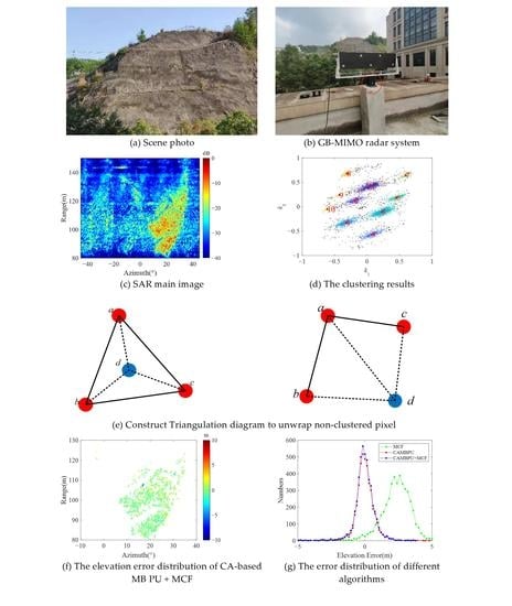
As shown in Figure 4, the connected graph of a non-clustered pixel includes two types. Figure 4a shows that a non-clustered pixel shown with a blue circle is inside a triangle, where the red circles denote the clustered pixels. In this case, the non-clustered pixel is directly connected to three vertices, and three small triangles are constructed. Figure 4b shows a non-clustered pixel that is outside the triangle. Two small triangles are constructed. It is worth noting that the shape of the triangle does not affect the accuracy of the phase unwrapping. Whether the accuracy is affected depends on whether the phase continuity assumption is satisfied between pixels. In addition, even if the unwrapping fails at this non-clustered pixel, the phase error will only be limited to this pixel and will not be propagated to other non-clustered pixels.
The following is the principle of a MCF phase unwrapping method suitable for an irregular network [20]. Give the network N = V , A , C , U , D , V is the set of residual pixels and node elements are usually represented by i or j . A is the set of arcs and i , j represents an arc from node i to node j . C is the weight function on the arc, also known as the unit cost, and c i j represents the unit cost of the arc. U is the upper bound for flow, and the lower bound of flow is zero. D is the supply and demand on the node, corresponding to the residual values −1, 0, 1. d i represents the supply and demand of node i . In this network, the network flow algorithm can calculate the flow x . x satisfies the following conditions:
min C x = ( i , j ) A c i j x i j s . t . j : ( i , j ) A x i j j : ( j , i ) A x j i = d i , i V
The network N with respect to flow x is defined as N x = V , A x , C x , U x , D , where the definitions of V and D remain unchanged. A x , C x , and U x are defined as follows:
A x = i , j | ( i , j ) A , x i j < u i j i , j | ( j , i ) A , x j i > 0
c i j x = c i j ( i , j ) A , x i j < u i j c j i ( j , i ) A , x j i > 0
u i j x = u i j x i j ( i , j ) A , x i j < u i j x j i ( j , i ) A , x j i > 0
From these, it can be shown that:
e i = d i + ( j , i ) A x j i ( i , j ) A x i j
where e i is the unbalanced number of nodes i . The initial value of e i is the supply and demand d i of node i . The purpose of the network flow algorithm is to construct a flow set with the smallest total cost. In Figure 4, select one of the three cluster pixels to integrate to obtain the absolute phase of the non-clustered pixel d according to the flow x .

5. Data Processing

5.1. Simulation Verification

Figure 5a shows the terrain of a steep cliff acquired with LiDAR which is utilized as the simulated dataset. The color represents the terrain height which changes from 50–250 m. Three interferograms acquired with baselines of 7 cm, 13 cm, and 17 cm are simulated. Moreover, Gaussian white noises with a standard deviation of 0.4 and mean value of 0 are added to these interferograms. Figure 5b–d show the interferometric fringes of different baselines, and the color axis represents the interferometric phase.
Figure 6 shows the clustering results. The red triangles in Figure 6a are the theoretical cluster centers and the blue pixels represent cross points with a cut plane in 3-D space according to (9). In Figure 6b, the red triangles represent the cluster centers obtained using DBSCAN, where different colors represent the pixels of different clusters and the black pixels are non-clustered pixels. A total of 10 cluster centers were obtained. Limited by the performance of the DBSCAN, a few pixels failed to cluster into groups.
The maximum difference between the unwrapped phase and the reference phase before filtering is 31.5646 rad. The maximum phase difference after filtering is 1.5102 rad. Denoising makes the clustering results more accurate. After subsequent processing, the unwrapped phase is obtained. Due to the longer baseline having better measurement accuracy, the unwrapped phase corresponding to the baseline of 17 cm is selected as the true phase. Finally, the elevation can be calculated using Equation (4) and the results are shown in Figure 7.
Figure 8 shows the elevation error of different algorithms. The MCF algorithm needs to select a reference pixel, so the result and the absolute phase may differ by an integer number of 2 π . After adding appropriate ambiguity numbers, the error distribution is shown in Figure 8a. It can be found that regional unwrapping failures exist on the left and right slopes. In Figure 8b, the elevation obtained by the CA-based MB PU algorithm is basically the same as the true elevation, but there are some isolated noise pixels. Figure 8c is the elevation error distribution with the improved algorithm, and there are fewer noise pixels compared to Figure 8b. The standard deviation of elevation error and the number of resulting pixels for the three algorithms are shown in Table 1. The MCF deals with all the PSs, but the standard deviation is also the largest at 12.0217 m. The standard deviation of the CA-based MB PU is smaller than that of MCF, but 6.2% of PS pixels are not unwrapped. Based on the CA-based MB PU, since the algorithm combines filtering and non-clustered pixel unwrapping, the standard is the smallest and the percentage of the unwrapped PSs reaches 99.3%. The accuracy of unwrapped PSs is defined as the proportion of unwrapped PSs with phase error less than π . Compared with SB PU, MB PU is quite robust to noise, so it has a higher accuracy for unwrapped PSs.

5.2. Experimental Data

5.2.1. Experimental Information

From 11:45 on 22 November 2021 to 14:27 on 22 November 2021 (China Standard Time), a GB-InSAR system was utilized to monitor an exposed slope (N29°40′58.99″, E106°47′0.49″) located in Chongqing City, China. As shown in Figure 9a, the slope is about 60 m long and 80 m wide, with an average thickness of 17.38 m.
The experiment uses a 16 × 16 FMCW (frequency-modulated continuous wave)-MIMO developed by Beijing Institute of Technology [21]. A picture of the system is shown in Figure 9b. The mechanical structure marked by the red circle can realize the baseline lengths of 7 cm, 13 cm, and 17 cm. The typical system parameters are summarized in Table 2.

5.2.2. Experimental Results

In this section, the DEM generated by GB-InSAR is compared with the DEM produced with high-precision LiDAR [22]. The LiDAR DEM is set as the true value, and the GB-InSAR DEM is estimated. Figure 10a is the main SAR image for the slope. With the method of amplitude dispersion and amplitude information (amplitude dispersion threshold is 0.15, amplitude information threshold is −18 dB), 5050 PSs are selected. The phase interferograms of different baselines are shown in Figure 10b–d.
As shown in Figure 11, a total of 10 clusters were obtained and black non-clustered pixels are distributed on the edge of each cluster.
Finally, the terrain generated by GB-InSAR is shown in Figure 12a and the terrain generated by LiDAR is shown in Figure 12b. The error results of the three unwrapping algorithms MCF, CA-based MB PU, and CA-based MB PU + MCF are shown in Figure 13. There is an overall offset in the elevation error due to the use of the MCF and the slope on the right failing to unwrap, resulting in error propagation. For the result with the CA-based MB PU, there are discrete isolated error pixels, and the error is distributed around zero. As is shown in Figure 13d, the method of CA-based MB PU + MCF has fewer error pixels and deals with more pixels.
From Table 3, we can see that the standard deviation of the elevation error with the CA-based MB PU + MCF method reaches 0.7429 m and this method deals with 98.2% of the PSs, which is 8.9% more than the CA-based MB PU method. The accuracy of MB PU is much greater than that of SB PU, and the accuracy of the CA-based MB PU + MCF is slightly larger than that of the CA-based MB PU. Although this improved method effectively solves the phase unwrapping problem, there is still some room for improvement. Compared with Figure 13b, there are few discrete error pixels in Figure 13c. This shows that error pixels concentrated at the position of 15°, 115 m still exist. SD-based DA shows good filtering performance for isolated and discrete noisy pixels but poor performance for regional noisy pixels. Secondly, non-clustered pixels are unwrapped by the SB PU method, which still needs to satisfy the phase continuity assumption.

6. Conclusions

A CA-based MB PU transforms the phase unwrapping problem into an unsupervised learning problem. However, due to noise, pixels affected by strong noise might deviate greatly from the true cluster centers and may not be accurately clustered. Therefore, this paper proposes an improved MB PU method which combines the advantages of the CA-based MB PU and MCF methods. Under the topological constraints of the triangulation network, the connectivity graph of any non-clustered pixel and its adjacent unwrapped cluster pixels can be established. Then, the absolute phase of any non-clustered pixel can be solved with the MCF method. This improved method overcomes the limitations of the Itoh and identifies the unwrapped phases of all PSs. In addition, the SD-based DA is utilized to filter out the isolated and discrete noisy pixels to further improve the phase unwrapping accuracy.
The performance of this improved method is evaluated by experiments. Compared with the DEM from LiDAR, the standard deviation of the measured elevation error is 0.7429 m, and this improved method unwraps 98.2% of the PSs with 99.01% accuracy of unwrapped PSs. Additionally, compared with the other two methods, this improved method has the smallest standard deviation. Experimental results demonstrate that this improved method is effective and quite robust to noise.

Author Contributions

Conceptualization, Z.L.; methodology, Z.L. and Y.D. (Yunkai Deng); validation, Z.L. and Y.D. (Yan Duan); investigation, Y.D. (Yan Duan) and W.T.; resources, W.T.; writing—original draft preparation, Z.L.; writing—review and editing, Y.D. (Yunkai Deng) and Z.Z.; supervision, W.T. and Y.D. (Yunkai Deng); funding acquisition, W.T. All authors have read and agreed to the published version of the manuscript.

Funding

This work was funded in part by National Key Research and Development Program of China under Grant 2021YFC3001903 and in part by the National Natural Science Foundation of China under Grants 62101036, 61971037, 31727901, and 61960206009.

Institutional Review Board Statement

Not applicable.

Informed Consent Statement

Not applicable.

Data Availability Statement

Not applicable.

Conflicts of Interest

The authors declare no conflict of interest.

References

  1. Pieraccini, M.; Miccinesi, L. Ground-Based Radar Interferometry: A Bibliographic Review. Remote Sens. 2019, 11, 1029. [Google Scholar] [CrossRef] [Green Version]
  2. Jung, H.S.; Won, J.S.; Kim, S.W. An Improvement of the Performance of Multiple-Aperture SAR Interferometry (MAI). IEEE Trans. Geosci. Remote Sens. 2009, 47, 2859–2869. [Google Scholar] [CrossRef]
  3. Kang, M.; Kim, K. Automatic SAR Image Registration via Tsallis Entropy and Iterative Search Process. IEEE Sens. J. 2020, 20, 7711–7720. [Google Scholar] [CrossRef]
  4. Jung, H.-S.; Lee, W.-J. An Improvement of Ionospheric Phase Correction by Multiple-Aperture Interferometry. IEEE Trans. Geosci. Remote Sens. 2015, 53, 4952–4960. [Google Scholar] [CrossRef]
  5. Kang, Y.; Lu, Z.; Zhao, C.; Zhang, Q.; Niu, Y. Diagnosis of Xinmo (China) Landslide Based on Interferometric Synthetic Aperture Radar Observation and Modeling. Remote Sens. 2019, 11, 1846. [Google Scholar] [CrossRef] [Green Version]
  6. Deng, Y.; Hu, C.; Tian, W.; Zhao, Z. 3-D Deformation Measurement Based on Three GB-MIMO Radar Systems: Experimental Verification and Accuracy Analysis. IEEE Geosci. Remote Sens. Lett. 2021, 18, 2092–2096. [Google Scholar] [CrossRef]
  7. Pieraccini, M.; Luzi, G.; Atzeni, C. Terrain mapping by ground-based interferometric radar. IEEE Trans. Geosci. Remote Sens. 2001, 39, 2176–2181. [Google Scholar] [CrossRef]
  8. Ghiglia, D.C.; Pritt, M. Two-Dimensional Phase Unwrapping: Theory, Algorithms, and Software; John Wiley & Sons, Inc.: Hoboken, NJ, USA, 1998. [Google Scholar]
  9. Yu, H.; Lan, Y.; Yuan, Z.; Xu, J.; Lee, H. Phase unwrapping in InSAR: A review. IEEE Geosci. Remote Sens. Mag. 2019, 7, 40–58. [Google Scholar] [CrossRef]
  10. Costantini, M. A novel phase unwrapping method based on network programming. IEEE Trans. Geosci. Remote Sens. 1997, 36, 813–821. [Google Scholar] [CrossRef]
  11. Itoh, K. Analysis of the phase unwrapping algorithm. Appl. Opt. 1982, 21, 2470. [Google Scholar] [CrossRef] [PubMed]
  12. Pascazio, V.; Schirinzi, G. Multifrequency InSAR height reconstruction through maximum likelihood estimation of local planes parameters. Image Process. IEEE Trans. 2002, 11, 1478–1489. [Google Scholar] [CrossRef]
  13. Ferraiuolo, G.; Pascazio, V.; Schirinzi, G. Maximum a posteriori height estimation in InSAR imaging. In Proceedings of the IEEE International Geoscience and Remote Sensing Symposium, Toronto, ON, Canada, 24–28 June 2002. [Google Scholar]
  14. Yu, H.; Li, Z.; Member, L.S.; Bao, Z. A Cluster-Analysis-Based Efficient Multibaseline Phase-Unwrapping Algorithm. IEEE Trans. Geosci. Remote Sens. 2010, 49, 478–487. [Google Scholar] [CrossRef]
  15. Rosen, P.A.; Hensley, S.; Joughin, I.R.; Li, F.K.; Madsen, S.N.; Rodriguez, E.; Goldstein, R.M. Synthetic aperture radar interferometry. Proc. IEEE 2002, 88, 333–382. [Google Scholar] [CrossRef]
  16. Noferini, L.; Pieraccini, M.; Mecatti, D.; Macaluso, G.; Luzi, G.; Atzeni, C. DEM by Ground-Based SAR Interferometry. IEEE Geosci. Remote Sens. Lett. 2007, 4, 659–663. [Google Scholar] [CrossRef]
  17. Ester, M.; Kriegel, H.P.; Sander, J.; Xu, X. A Density-Based Algorithm for Discovering Clusters in Large Spatial Databases with Noise. In Proceedings of the KDD’96: Proceedings of the Second International Conference on Knowledge Discovery and Data Mining, Portland, OR, USA, 2–4 August 1996; Volume 96, pp. 226–231. [Google Scholar]
  18. Deng, Y.; Tian, W.; Xiao, T.; Hu, C.; Yang, H. High-Quality Pixel Selection Applied for Natural Scenes in GB-SAR Interferometry. Remote Sens. 2021, 13, 1617. [Google Scholar] [CrossRef]
  19. Rusu, R.B.; Blodow, N.; Marton, Z.C.; Soos, A.; Beetz, M. Towards 3D object maps for autonomous household robots. In Proceedings of the 2007 IEEE/RSJ International Conference on Intelligent Robots and Systems, San Diego, CA, USA, 29 October–2 November 2007. [Google Scholar]
  20. Yong, Y.U.; Wang, C.; Zhang, H.; Liu, Z.; Gao, X. A Phase Unwrapping Method Based on Network Flow Algorithm in Irregular Network. J. Remote Sens. 2003, 7, 472–477. [Google Scholar]
  21. Cheng, H.U.; Deng, Y.; Tian, W. Multistatic ground-based differential interferometric MIMO radar for 3D deformation measurement. Sci. China Inf. Sci. 2021, 64, 2. [Google Scholar]
  22. Tian, W.; Zhao, Z.; Hu, C.; Wang, J.; Zeng, T. GB-InSAR-Based DEM Generation Method and Precision Analysis. Remote Sens. 2019, 11, 997. [Google Scholar] [CrossRef] [Green Version]
Figure 1. Geometric schematic of GB-InSAR measurement.
Remotesensing 14 02543 g001
Figure 2. Straight lines corresponding to ambiguity vectors with k 1 as its abscissa and k 2 as its ordinate. (a) Straight lines in the absence of noise. (b) Straight lines in the presence of noise.
Remotesensing 14 02543 g002
Figure 3. Processing flow of the improved method.
Remotesensing 14 02543 g003
Figure 4. Triangulation diagram. (a) Inside the triangle. (b) Outside the triangle.
Remotesensing 14 02543 g004
Figure 5. Simulated topography and interferograms of different baselines. (a) Simulated topography, (b) 7 cm baseline, (c) 13 cm baseline, and (d) 17 cm baseline.
Remotesensing 14 02543 g005
Figure 6. The clustering results. (a) Theoretical cluster center. (b) The clustering results.
Remotesensing 14 02543 g006
Figure 7. The height of all PSs. (a) Top view. (b) 3-D view.
Remotesensing 14 02543 g007
Figure 8. The Elevation error distribution of different algorithms. (a) MCF. (b) CA-based MB PU. (c) CA-based MB PU + MCF.
Remotesensing 14 02543 g008
Figure 9. Experimental information. (a) Scene photo. (b) GB-MIMO radar system.
Remotesensing 14 02543 g009
Figure 10. SAR images and interferograms of different baselines. (a) SAR main image, (b) 7 cm baseline, (c) 13 cm baseline, and (d) 17 cm baseline.
Remotesensing 14 02543 g010aRemotesensing 14 02543 g010b
Figure 11. The clustering results.
Remotesensing 14 02543 g011
Figure 12. DEMs. (a) DEM generated by GB-InSAR. (b) DEM generated by LiDAR.
Remotesensing 14 02543 g012
Figure 13. The elevation error distribution of different algorithms. (a) MCF. (b) CA-based MB PU. (c) CA-based MB PU + MCF. (d) Error distribution.
Remotesensing 14 02543 g013
Table 1. Different algorithm processing results.
AlgorithmStandard Deviation of Elevation Error (m)Percentage of Unwrapped PSsThe Accuracy of Unwrapped PSs
MCF algorithm12.0217100%91.74%
CA-based MB PU5.832193.8%99.6%
CA-based MB PU + MCF 1.901599.3%100%
Table 2. Technical characteristics of GB-MIMO radar.
ParameterValueParameterValue
Central frequency16.2 GHzBandwidth400 MHz
Transmitting channels16Receiving channels16
Range resolution0.375 mAzimuth resolution7.4 mrad
Table 3. Different algorithms’ processing results.
AlgorithmStandard Deviation of Elevation Error (m)Percentage of Unwrapped PSsThe Accuracy of Unwrapped PSs
MCF algorithm2.2581100%58.61%
CA-based MB PU1.135689.3%98.45%
CA-based MB PU + MCF 0.742998.2%99.01%
Publisher’s Note: MDPI stays neutral with regard to jurisdictional claims in published maps and institutional affiliations.

