High-Precision Joint Magnetization Vector Inversion Method of Airborne Magnetic and Gradient Data with Structure and Data Double Constraints

Abstract

Airborne magnetic and gradient measurements are commonly used geophysical remote sensing tools to obtain the distribution features of ore mineral bodies. It is known that ore mineral bodies generally contain remanent magnetization, and magnetization vector inversion (MVI) can produce the magnetization intensity and direction of the source, which is more suitably used to interpret measured airborne magnetic and gradient data. To accurately reveal the underground magnetization vector distribution, we proposed a high-precision method with double constraints on the data and physical structure, and we used the cross-gradient inversion of airborne magnetic anomalies and the combination matrix of airborne magnetic and gradient (CMG) data to recover the physical parameters of the sources with different depths. We used the combination matrix to produce the different component data constraints and the cross-gradient function to finish the inversion to provide structural constraints. For anomaly sources at similar depths, joint inversion based on the cross-gradient of magnetic gradient data and CMG data is more suitably used. The superiority of the double constraints method is proven by theoretical model tests. We apply the proposed method to interpret airborne magnetic and gradient data in Shandong Province to detect iron mineral resources, and we select the cross-gradient inversion of airborne magnetic anomalies and CMG data depending on the nonlinear features of the power spectrum. The main ore bodies have a northeast distribution with a depth range of 1048–1800 m, successfully giving the distribution range of the high-magnetic bodies; a better mineral potential is in the northern part of the survey area.

1. Introduction

Airborne magnetic measurement is an effective remote sensing geophysical method to detect magnetic ore resources. Compared to airborne magnetic data, airborne magnetic gradient data can effectively strengthen shallow sources and have higher horizontal resolution, while airborne magnetic data can better retain the information of deep sources [1,2,3,4,5,6,7,8]. Thus, joint exploration of airborne magnetic and magnetic gradient data is often used to obtain the anomaly characteristics of sources with different depths [9]. Besides, the joint inversion of different types of airborne magnetic data with other geophysical datasets has been widely used in quantitative interpretation of airborne magnetic data. More accurate interpretation results can be obtained by combining geophysical datasets [10,11,12].

The inversion of magnetic bodies includes the position and physical properties. We have the calculation methods of the center of field source such as normalized source strength (NSS), analytic signal (AS), and local wavenumbers [13,14,15,16,17,18,19]. Moreover, many inversion algorithms based on the Tikhonov regularization have been developed to obtain physical parameters (susceptibility values and burial depth) of the magnetic bodies [20,21,22,23,24].

Natural remanent magnetization of rocks is commonly existent; therefore, the magnetization vector inversion is more suitable for the inversion of magnetic data influenced by remanent magnetization, which can obtain the magnetization intensity and direction of the sources [25,26,27,28,29,30,31]. Lelièvre and Oldenburg [25] first proposed the MVI method, which effectively handled inversions with Cartesian and spherical coordinate systems. Liu et al. [28] accomplished the 2D MVI of well magnetic data and studied the influence of remanence and demagnetization.

MVI requires an accurate initial value of the magnetization direction [32,33,34,35,36]. The analytic signal and normalized source strength are weakly sensitive to the magnetization direction, so it is more suitable to estimate the magnetization direction of the field source by calculating its correlation with the reduction to the pole anomalies at different angles [37].

Currently, the joint inversion of airborne magnetic and magnetic gradient data mainly uses the data constraint method, which combines airborne magnetic anomalies and gradient anomalies into the same data matrix to obtain a more accurate underground magnetic structure by meeting the fitting accuracy of different component data [9].

The precise magnetization direction of an underground structure is of great importance to interpret magnetic data. In this paper, the MID (magnetization intensity M, inclination I, declination D) inversion method was adopted [28]. Based on the existing data constraint method of CMG data, aiming at the distribution characteristics of underground field sources, we propose a high-precision joint inversion method with double constraints of data and physical structure; CMG data is used to produce the data constraint to complete MID inversion; the cross-gradient function provides structural constraints to finish the MID inversion. The proposed double constraints inversion method can better obtain the accurate distribution of the sources. The superiority of the proposed method is verified by model tests.

2. Methods

2.1. Previous Inversion Method

The MID inversion of the magnetic field and its gradient combines different data in a matrix; objective function of the data constraint inversion based on the Tikhonov regularization method can be expressed as:

$${\varphi }_1=\parallel W_d\left[\begin{array}{c}\begin{array}{ccc}{G}_M^{\Delta T}& G_I^{\Delta T}& G_D^{\Delta T}\end{array}\\ \begin{array}{ccc}{G}_M^{\Delta T_z}& G_I^{\Delta T_z}& G_D^{\Delta T_z}\end{array}\end{array}\right]\left[\begin{array}{c}\Delta M\\ \Delta I\\ \Delta D\end{array}\right]-\left[\begin{array}{c}\Delta T\\ \Delta T_z\end{array}\right]{\parallel }_2^2+\mu \parallel W\left[\begin{array}{c}\Delta M\\ \Delta I\\ \Delta D\end{array}\right]{\parallel }_2^2,$$

(1)

where ${\varphi }_1$ represents the objective function of the CMG data; $G_M^{\Delta T}$ and $G_M^{\mathsf{\Delta }{T}_z}$ represent the kernel matrix of airborne magnetic and gradient data, respectively; $G_I^{\Delta T}$ and $G_I^{\Delta T_z}$ represent the kernel function matrix of the magnetization inclination correction of airborne magnetic and gradient anomaly, respectively; $G_D^{\Delta T}$ and $G_D^{\Delta T_z}$ represent the kernel function matrix of the magnetization declination correction of airborne magnetic and gradient anomaly, respectively; $\Delta T$ and $\Delta T_z$ represent airborne magnetic and gradient data, respectively. μ is the regularization coefficient; W_d is the data-weighing matrix [22]; ΔM, ΔI and ΔD are the corrections of magnetization intensity, inclination and declination; and W is the weighted matrix composed of three diagonal matrices and can be written as:

$$W=\left[\begin{array}{ccc}{W}_M& 0& 0\\ 0& W_{I}E& 0\\ 0& 0& W_{D}E\end{array}\right]$$

(2)

where W_M, W_I+, and W_D represent weighted coefficients of the magnetization intensity, inclination, and declination, respectively; E is the unit matrix; I₀ and D₀ represent initial model of inclination and declination, respectively; the initial values of I₀ and D₀ will be determined by the correlation coefficients between the analytical signal (AS) of the data and the anomalies after reducing to the pole at different angles [35], and the equation for calculating the correlation coefficient is given by:

$$C\left(I_0,D_0\right)=\frac{{{\displaystyle \sum }}_k\left(A{S}_k-\overline{AS}\right)\left(v_{\perp k}-\overline{v_{\perp }}\right)}{{{\displaystyle \sum }}_k{(A{S}_k-\overline{AS})}^2{(v_{\perp k}-\overline{v_{\perp }})}^2},$$

(3)

To improve the efficiency of calculation, P was brought into the solution expression of Equation (1); P is the preconditioned matrix, and the specific expression is:

$$P=\left[\begin{array}{ccc}{z}^{\beta }& 0& 0\\ 0& E& 0\\ 0& 0& E\end{array}\right],$$

(4)

where z is the depth of burial and β (β ≤ 6) is a constant related to the rapid attenuation of the magnetic anomaly with the distance between the observation points and the field sources [23,27]; β is generally 3.

We use the anomalies of the synthetic model of two prisms with different depths to test the MID inversion effect of data constraint. Figure 1a shows the synthetic magnetic anomaly and its gradient anomaly of two prisms with locations of (550, 1000, and 350) m and (1450, 1050, and 650) m. The magnetization inclination and declination angles are 45°, and inclination and declination of the Earth’s magnetic field angles are 50°; and the magnetization intensity is 5 A/m. In this paper, the total magnetization direction of the underground field source is calculated.

Figure 1b,c show the estimated magnetization inclination and declination by Equation (3), and they are 5°–42° and 30°–40°, with averages of 37° and 39°, respectively. The magnetization inclination values vary more, and the range of magnetization declination is relatively narrow. These are used as the initial values for MID inversion and the inversion results is converged with RMS errors reaching 0.03 nT and 0.12 nT/m.

Figure 1d shows the results of synthetic magnetic anomaly under natural conditions by the Tikhonov regularization method. For simplicity, the result of susceptibility is transformed to magnetization intensity; For the inversion results under natural conditions, we have all done the same transformation. It shows that the range of the geological bodies is divergent and the response of the shallow source is weak.

Figure 1e shows the MID inversion results of the synthetic magnetic anomaly. The blue arrows represent the recovered magnetization direction, and the estimated values of magnetization inclination and declination are 36.3°–52.4° and 38.6°–41.3°, with averages of 39.9° and 40.5°, respectively. Compared with the result under natural conditions, the inversion result of magnetization intensity shows the position of the shallower prism precisely, while the deep source is not convergent. The inversion result of the range of magnetization inclination is more orderly than the initial values, the improvement of magnetization declination is not obvious, and the average of them is closer to the real value compared with the initial values.

Figure 1f shows the MID inversion result of the synthetic magnetic gradient anomaly, and the estimation results of magnetization inclination and declination are 37.2°–60.0° and 39.1°–41.3°, with averages of 38.5°and 39.5°, respectively. The horizontal resolution of the magnetization intensity inversion result has been significantly improved, and the reconstruction ability of the deep field source is still poor. Moreover, the range of magnetization inclination is larger than that of the magnetic anomaly, the results of magnetization declination are close to the results of the magnetic anomaly, and their averages are consistent with the results of Figure 1e.

Figure 1g shows the MID inversion result of the CMG data, and the estimation results of magnetization inclination and declination are 36.3°–55.8° and 39.2°–41.3°, with averages of 39.5° and 40.0°, respectively. The recovery of the shallow source and the convergence of the deep source are better than the MID inversion result of the magnetic anomaly. The recovery of the deep source amplitude is better than the MID inversion result of the magnetic gradient anomaly. However, there is still a deviation between the deep field source and the real value. The magnetization inclination and declination are similar to the other results.

Compared with the above results, the improvement of vertical resolution by the data constraint method is limited, and the deviation between the estimated values of the magnetization inclination of the airborne magnetic anomaly and the real value is smaller than that of synthetic magnetic anomaly and its gradient anomaly.

The attenuation curve of the eigenvalue spectra can characterize the ability to recover the distribution of sources using different types of data and can be expressed as:

$$G=U\Sigma V,$$

(5)

where U and V represent the left vector matrix and right vector matrix, respectively, and Σ represents the singular value matrix of different types of data. The high frequency and low frequency of the eigenvalue spectra correspond to the deep and shallow parts of the sources, respectively. The larger the eigenvalue spectra are, the better the recovery ability of the corresponding data to the sources [38]. Figure 1h shows the eigenvalue spectra of synthetic magnetic gradient anomaly and CMG anomaly. It can be seen that the combination of synthetic magnetic and magnetic gradient anomaly data recovers deep sources better than single data, and it also proves that multitype data combinations can improve the accuracy of inversion results.

Cross-gradient function rely on gradient-based relationship, it is often used in the joint inversion [39,40,41,42,43], and the corresponding objective function of the cross-gradient method can be expressed as:

$${\varphi }_2=\parallel W_d\left[\begin{array}{ccc}{G}_M^{\Delta T}& G_I^{\Delta T}& G_D^{\Delta T}\end{array}\right]\left[\begin{array}{c}\Delta M\\ \Delta I\\ \Delta D\end{array}\right]-\left[\Delta T\right]{\parallel }_2^2+\mu \parallel W\left[\begin{array}{c}\Delta M\\ \Delta I\\ \Delta D\end{array}\right]{\parallel }_2^2+{\lambda }_{\Delta T}{\Phi }_{cross},$$

(6)

$${\varphi }_3=\parallel W_d\left[\begin{array}{ccc}{G}_M^{\Delta T_z}& G_I^{\Delta T_z}& G_D^{\Delta T_z}\end{array}\right]\left[\begin{array}{c}\Delta M\\ \Delta I\\ \Delta D\end{array}\right]-\left[\Delta T_z\right]{\parallel }_2^2+\mu \parallel W\left[\begin{array}{c}\Delta M\\ \Delta I\\ \Delta D\end{array}\right]{\parallel }_2^2+{\lambda }_{\Delta T_z}{\Phi }_{cross},$$

(7)

where ${\varphi }_2$ and ${\varphi }_3$ are the objective functions of the airborne magnetic anomaly and airborne magnetic gradient anomaly, respectively, and ${\lambda }_{\Delta T}$ is the coefficients of the cross-gradient terms of magnetic data; ${\lambda }_{T_z}$ is the coefficients of the cross-gradient terms of airborne magnetic gradient data. ${\Phi }_{cross}$ is the cross-gradient function of airborne magnetic data and gradient data. Figure 1i shows the inversion result of the airborne magnetic anomaly by the structure constraint method. Figure 1j shows the inversion result of the airborne magnetic gradient anomaly by the structure constraint method, and the magnetization inclination and declination are 36.3°–49.8° and 39.2°–41.3°, with averages of 42.5° and 39.7°, respectively. Compared with the MID inversion results, the structure constraint method obtains higher vertical resolution, but the horizontal resolution is blurry, and the response of the deep source is still weak; the range of magnetization inclination is further reduced and closer to the true value than the above results, and the increase of magnetization declination is similar to the above results.

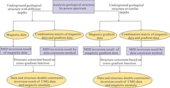
2.2. Double Constraints Inversion Method of Data and Structure

To improve the recovery effect for deep sources, we propose a joint inversion method with double constraints of data and structure, which uses the cross gradient of CMG data and airborne magnetic data to complete the MID inversion; anomalies caused by the sources with different depths; the objective function can be expressed as:

$${\varphi }_4={\Vert W_d\left[\begin{array}{c}\begin{array}{ccc}{G}_M^{\Delta T}& G_M^{\Delta T}& G_M^{\Delta T}\end{array}\\ \begin{array}{ccc}{G}_M^{\Delta T_z}& G_M^{\Delta T_z}& G_M^{\Delta T_z}\end{array}\end{array}\right]\left[\begin{array}{c}\Delta M\\ \Delta I\\ \Delta D\end{array}\right]-\left[\begin{array}{c}\Delta T\\ \Delta T_z\end{array}\right]\Vert }_2^2+\mu {\Vert W\left[\begin{array}{c}\Delta M\\ \Delta I\\ \Delta D\end{array}\right]\Vert }_2^2+{\lambda }_{T{T}_z}{\Phi }_{crossT{T}_z},$$

(8)

$${\varphi }_5={\Vert W_d\left[\begin{array}{ccc}{G}_M^{\Delta T}& G_I^{\Delta T}& G_D^{\Delta T}\end{array}\right]\left[\begin{array}{c}\Delta M\\ \Delta I\\ \Delta D\end{array}\right]-\left[\Delta T\right]\Vert }_2^2+\mu {\Vert W\left[\begin{array}{c}\Delta M\\ \Delta I\\ \Delta D\end{array}\right]\Vert }_2^2+{\lambda }_{\Delta T}{\Phi }_{crossT{T}_z},$$

(9)

where ${\varphi }_4$ represents the objective function of the CMG data with the constraint of airborne magnetic data; ${\varphi }_5$ represents the objective function of the airborne magnetic data with the constraint of CMG data; and ${\Phi }_{crossTTz}$ is the cross-gradient function of airborne magnetic data and CMG data. We obtain the final results with Equation (8) to distinguish geological bodies of different depths; this method can effectively realize the joint inversion of double constraints of data and structure; the specific calculation process shows in Figure 2.

Since the inversion result of airborne magnetic gradient data has higher horizontal resolution, for sources with similar depths, we use the cross-gradient constraint of airborne magnetic gradient data and the CMG data to obtain the distribution of the sources. The objective function can be expressed as:

$${\varphi }_6=\parallel W_d\left[\begin{array}{c}\begin{array}{ccc}{G}_M^{\Delta T}& G_M^{\Delta T}& G_M^{\Delta T}\end{array}\\ \begin{array}{ccc}{G}_M^{\Delta T_z}& G_M^{\Delta T_z}& G_M^{\Delta T_z}\end{array}\end{array}\right]\left[\begin{array}{c}\Delta M\\ \Delta I\\ \Delta D\end{array}\right]-\left[\begin{array}{c}\Delta T\\ \Delta T_z\end{array}\right]{\parallel }_2^2+\mu \parallel W\left[\begin{array}{c}\Delta M\\ \Delta I\\ \Delta D\end{array}\right]{\parallel }_2^2+{\lambda }_{T{T}_z}{{\Phi }^{\prime }}_{crossT{T}_z},$$

(10)

$${\varphi }_7=\parallel W_d\left[\begin{array}{ccc}{G}_M^{\Delta T_z}& G_I^{\Delta T_z}& G_D^{\Delta T_z}\end{array}\right]\left[\begin{array}{c}\Delta M\\ \Delta I\\ \Delta D\end{array}\right]-\left[\Delta T_z\right]{\parallel }_2^2+\mu \parallel W\left[\begin{array}{c}\Delta M\\ \Delta I\\ \Delta D\end{array}\right]{\parallel }_2^2+{\lambda }_{\Delta T_z}{{\Phi }^{\prime }}_{crossT{T}_z}$$

(11)

where ${\varphi }_6$ represents the objective function of the CMG data with the airborne magnetic gradient data constraint and ${\varphi }_7$ represents the objective function of the airborne magnetic gradient data with the constraint of CMG data. ${{\Phi }^{\prime }}_{crossTTz}$ is the cross-gradient function of airborne magnetic data and CMG data. The final inversion results obtained by Equation (10) can precisely recover the distribution of geological bodies with similar depths, proving that our method has applicability.

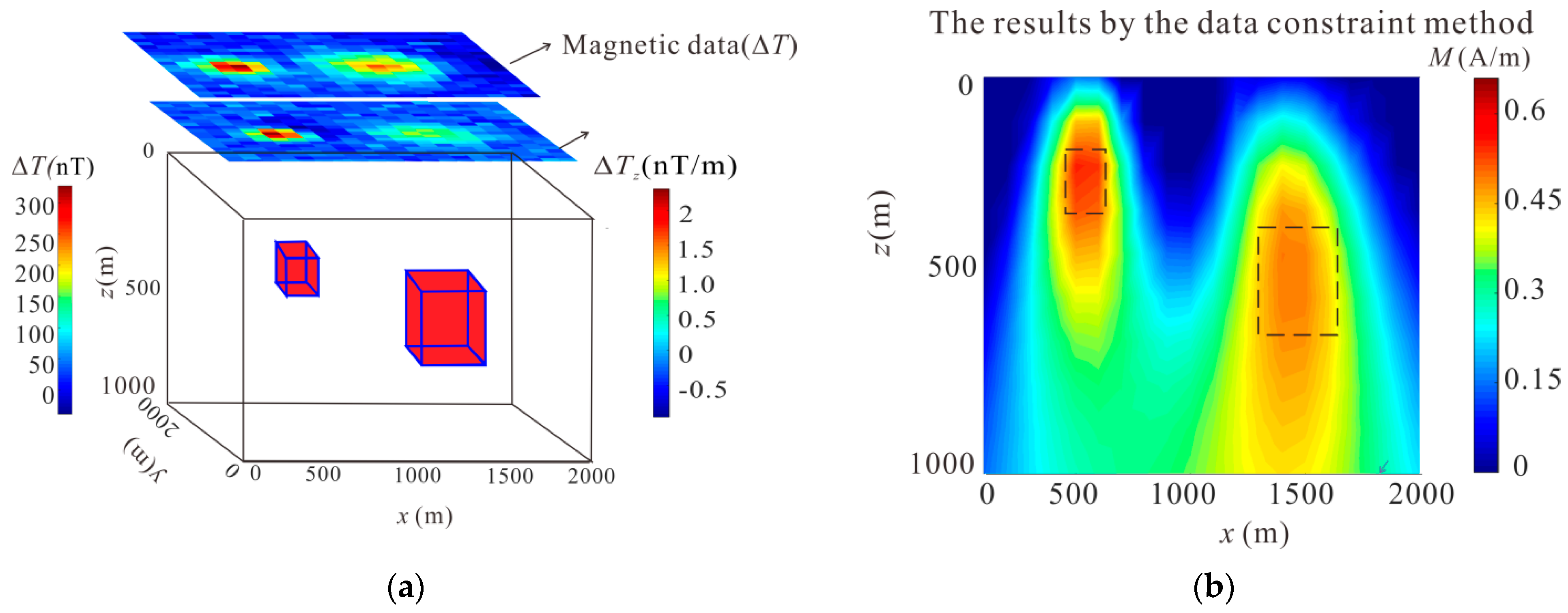
3. Theoretical Model Tests

We perform experiments on joint inversion with double constraints of data and structure. Figure 3a shows the CMG data result by the double constraints inversion method of magnetic gradient anomaly and CMG data, and the magnetization inclination and declination are 36.3°–49.8° and 39.2°–41.3°, with averages of 42.5° and 39.7°, respectively. Figure 3b shows the corresponding 3D magnetization vector view with a cutoff display value of 0.471 A/m. Comparing the results of the structure constraint method and data constraint method, the horizontal resolution and convergence of the result in Figure 3a are significantly improved. However, the result still deviates from the deep source, and the results of the magnetization direction are consistent with the results of the structure constraint method. Figure 3c shows the CMG data result by the double constraints inversion method of magnetic anomaly and CMG data, and the magnetization inclination and declination are 36.3°–49.8° and 39.2°–41.3°, with averages of 42.5° and 39.7°, respectively. Figure 3d shows the corresponding 3D magnetization vector view with a cutoff value of 0.471 A/m. Compared with the above results, the magnetization intensity in Figure 3c can accurately recover the distribution of sources, and it can also be seen that the double constraint result of the magnetization direction is the same as the results of the structural constraint. Thus, magnetization direction is not the key research goal, and the following is mainly aimed at improving resolution.

In practice, the aeromagnetic survey interference is approximately 3~5 nT. To verify the anti-noisy nature of the method in this paper, Gaussian noise with a mean of 4 nT is added to the anomalies in Figure 1a. Figure 4a shows the noise-corrupted airborne magnetic anomaly and its gradient anomaly. Gaussian noise obviously affects the shape of airborne magnetic gradient data. Figure 4b shows the MID inversion result by the data constraint method. The inversion result of magnetization intensity shows that the data constraint inversion method has good anti-noisy properties, but the horizontal resolution is low. Figure 4c shows the CMG data result by the double constraint inversion of the airborne magnetic anomaly and CMG data. Figure 4d shows the corresponding 3D magnetization vector view of CMG data with a cutoff display value of 0.471 A/m. Comparing the results in Figure 4b, the magnetization intensity results have higher anti-noise and resolution. This proves that our method can still reconstruct the position and depth of the sources.

We set sources with similar depths to test the application of the inversion method with double constraints of data and structure. Figure 5a shows the airborne magnetic field and its gradient anomaly of two prisms with locations of (750, 1000, and 350) m and (1450, 1000, and 350) m. The magnetization inclination and declination angles are 45°, and inclination and declination of the Earth’s magnetic field angles are 50°; and the magnetization intensity is 5 A/m. The correlation coefficient method of Equation (3) is used to calculate the initial values of magnetization inclination and declination of the sources, which are 5°–42° and 30°–40°, with averages of 36° and 39°, respectively.

To synthetic model with similar depth, Figure 5b shows the result under natural conditions by the Tikhonov regularization method; it shows that the shape of geological bodies distort without regard to remanent magnetization. Figure 5c shows the MID inversion result by the data constraint method; compared with the result of Figure 5b, the boundary of the result is fuzzy, and the resolution of the data constraint is weak. Figure 5d shows the CMG data result by the double constraints inversion method of magnetic anomaly and CMG data. Figure 5e shows the corresponding 3D magnetization vector view with a cutoff value of 0.60 A/m. Comparing the result in Figure 5c, the vertical resolution is significantly improved, whereas a difference is seen in magnetization intensity amplitude between the inversion result and setting value. Figure 5f shows the CMG data result by the double constraints inversion method of the airborne magnetic gradient anomaly and CMG data. Figure 5g shows the corresponding 3D magnetization vector view with a cutoff value of 0.60 A/m. By comparing with the result in Figure 5d, the inversion of magnetization intensity in Figure 5f is consistent with the underground distribution, and it has a higher resolution. Thus, we have proved that the double constraints inversion method of airborne magnetic gradient anomalies and CMG data is more suitable for sources with similar depths.

We verified the applicability of our method when the direction of the sources differs greatly. We set the magnetization direction of the shallow source as (I₁, D₁) = (45°, 45°) and the magnetization direction of the deep source as (I₂, D₂) = (60°, 45°) in Figure 1a. The correlation coefficient method of Formula 3 was used to calculate the initial values of magnetization inclination and declination of the sources, which were 10°–48° and 30°–40°, with averages of 50° and 39°, respectively. The existence of remanent magnetization complicates the inversion problem. Figure 6b shows the inversion result by the data constraint method without regard to remanent magnetization. The inversion result shows that the shape of the sources is significantly affected by the remanent magnetization. Therefore, it is unreasonable to calculate the magnetization under natural conditions when airborne magnetic data is affected by remanent magnetization. Figure 6c shows the CMG data result by the double constraints inversion method with Equation (8). Figure 6d shows the corresponding 3D magnetization vector view with a cutoff display value of 0.471 A/m. Compared with the result in Figure 6b, the double constraints inversion method can better reconstruct the physical parameters, which include the magnetization intensity and direction of the sources, in higher resolution. The magnetization inclination and declination are 48.2°–62.8° and 39.2°–42.5°, respectively, with averages of 50.5° and 39.7°, respectively, and they are similar to the real values. Thus, we have proved that our method is still suitable for sources with different magnetization directions.

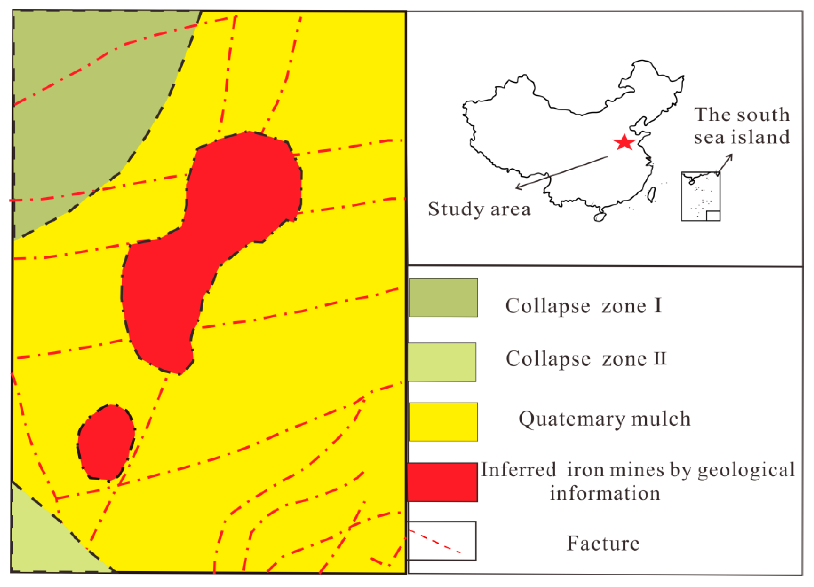
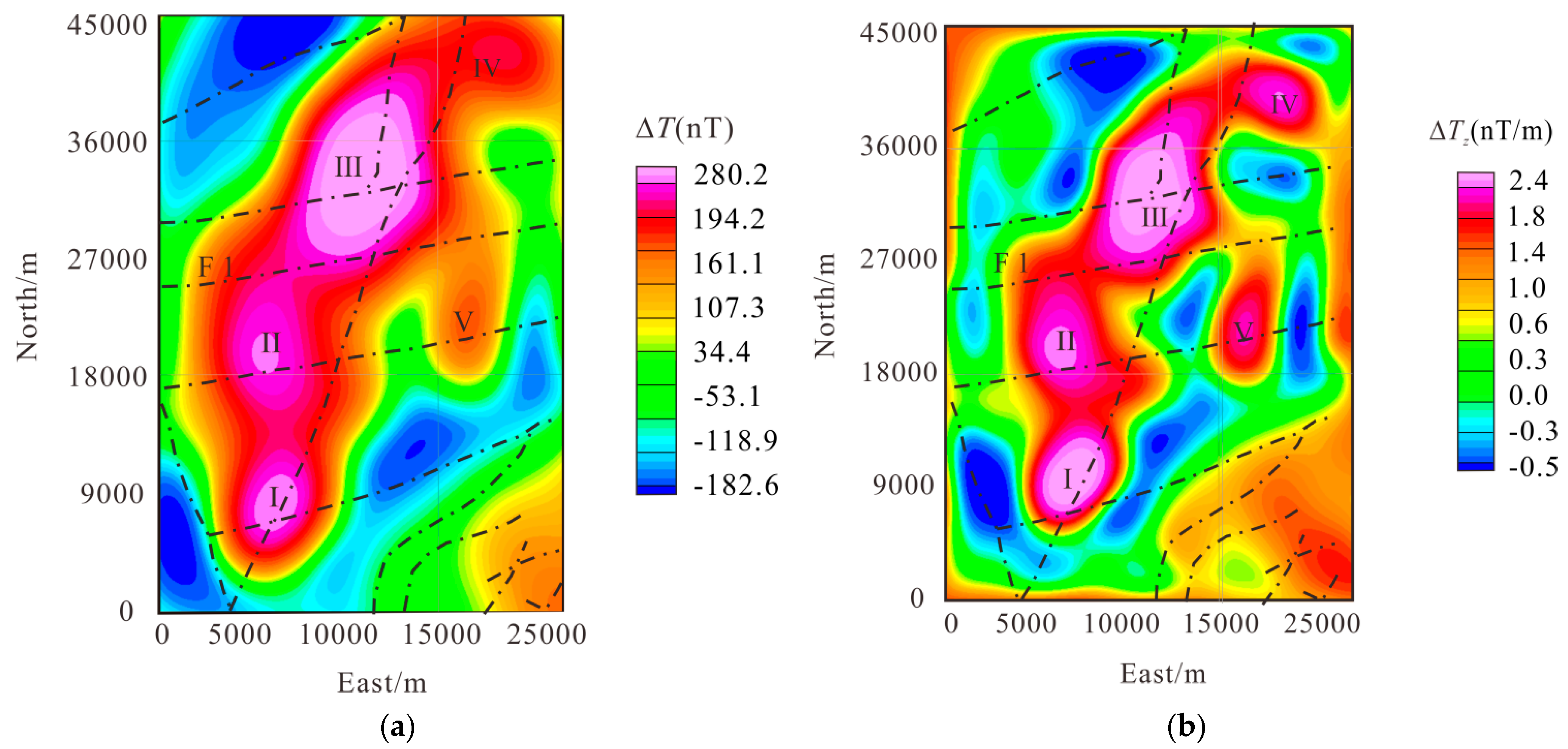
4. Field Data Application

The average thickness of the Cenozoic in an area of Shandong Province is more than 800 m. Figure 7 shows the geological conditions. The strikes of the fault are widely distributed, including NE and SN. There are granite and ferromagnetic ore bodies; the ferromagnetic ore bodies all occur in the contact zones between the Late Yanshan intermediate complex and the Ordovician Majiagou carbonate rock [44].

To obtain the distribution characteristics of iron ore bodies, we carried out a 1: airborne magnetic survey in the area, and the vertical gradient data were obtained by the difference of the magnetic data at two different heights by conducting repeated flights. Flight line direction is nearly NS and tie line direction is SN. Figure 8a,b are airborne magnetic and gradient anomalies, respectively. There are three main high-value regions in Figure 8a and five high-value regions in Figure 8b, and there is a good correspondence between the high values of anomalies and the high-magnetic bodies; the fault (F1) causes dislocation of high-magnetic bodies II and III. A magnetic gradient anomaly can obtain more details of underground geological structures and be more sensitive to the shallower geological structures [5]. Compared with Figure 8a, Figure 8b shows a more obvious boundary of high magnetic bodies IV and V, with higher resolution. Meanwhile, spectral analysis of airborne magnetic anomaly is conducted to analyze the underground structure in the research area, as shown in Figure 9. The relationship between power spectrum and buried depth of the geological bodies is non-linear; according to the power spectrum curve [45], we infer that high-magnetic bodies IV and V are obvious and are shallower compared with high-magnetic bodies I, II, and III. Thus, we use cross gradient inversion of the magnetic data and CMG data to obtain the distribution of high-magnetic bodies.

Figure 10a shows airborne magnetic and magnetic gradient data and the location of the borehole. The correlation coefficient method of Equation (3) is used to calculate the initial values of magnetization inclination and declination of the sources, and they are 40°–50° and −1.6°–2.5°, respectively. Slices of the double constraints inversion results of airborne magnetic data and CMG data are shown in Figure 10b. The results indicate that there are three major high-magnetic bodies (I, II, and III), and the top depth of high-magnetic bodies I and II is approximately 1100 m, with a thickness of approximately 400 m; high-magnetic body III is bigger than the other high-magnetic bodies, with a top depth of 1200 m and a thickness of approximately 600 m. The size of some magnetic bodies is small, with magnetic bodies IV and V having depth ranges of 1048–1108 m and 1048–1260 m, respectively. Figure 10c is a borehole laid in the magnetic bodies (I and III) during exploration, with coordinates of (28,000 mm, 10,000 m). A high-magnetic skarn is found at 1157 m depth, where the magnetization intensity is up to 35.1 A/m; a high-magnetic skarn is covered on monzonitic granite and diorite [46], which verifies the correctness of the inversion results. Figure 10d is a three-dimensional result of the magnetization intensity larger than 12.8 A/m and corresponds to the distribution of the horizontal range, according to the position of the highly magnetic body in the borehole. Moreover, it is shown that the north and south of high-magnetic body III have obviously different magnetization directions. We speculate that it formed because of the subduction of the Pacific plate to the Eurasian plate, and it can be seen that the method in this paper obtains the specific distribution of high-magnetic bodies (I, II, and III) as a favorable target for subsequent exploration.

5. Discussion and Conclusions

We proposed a data and structure double constraints method of airborne magnetic and magnetic gradient data; different types of magnetic data are used as data constraints and cross-gradient functions are used as structural constraints. This can effectively improve the accuracy of magnetic and gradient joint inversion.

The model tests show that the proposed method is more effective in reconstructing the physical parameters (depth, size, and magnetization direction) of the synthetic field source. Compared with MID inversion, the proposed method improves the magnetization intensity by 0.2 nT, and the obtained magnetization inclination is about 2.5 degrees higher than the MID inversion method; it is confirmed that the data and structure double constraints inversion method of airborne magnetic data and CMG data is more suitable for sources with different depths, and the data and structure double constraints method of airborne magnetic gradient data and CMG data is suitable for models with similar depths.

In view of the distribution of high-magnetic bodies in Shandong Province, we carry out joint inversion of the magnetic data and magnetic gradient data and obtain the magnetization intensity and direction of high-magnetic bodies, which points out the direction for subsequent exploration. Finally, the causes of obviously different magnetization directions of high-magnetic bodies in this area are analyzed, which provides important basic data for the study of regional mineral genesis.

References

1. Nelson, J.B. Calculation of the magnetic gradient tensor from total field gradient measurements and its application to geophysical interpretation. Geophysics 1988, 53, 957–966. [Google Scholar] [CrossRef]
2. Schmidt, P.W.; Clark, D.A. The magnetic gradient tensor: Its properties and uses in source characterization. Lead. Edge 2006, 25, 75–78. [Google Scholar] [CrossRef] [Green Version]
3. Yang, Y.S.; Li, Y.Y.; Liu, T.Y.; Zhang, Y.L.; Feng, X. Interactive 3D forward modeling of total field surface and three-component borehole magnetic data for the Daye iron-ore deposit (Central China). J. Appl. Geophys. 2011, 75, 254–263. [Google Scholar] [CrossRef]
4. Beiki, M.; Clark, D.A.; Austin, J.R.; Foss, C.A. Estimating source location using normalized magnetic source strength calculated from magnetic gradient tensor data. Geophysics 2012, 77, J23–J37. [Google Scholar] [CrossRef] [Green Version]
5. Ren, Z.Y.; Chen, C.Y.; Tang, J.T.; Chen, H.; Hu, S.G.; Zhou, C.; Xiao, X. Closed-form formula of magnetic gradient tensor for a homogeneous polyhedral magnetic target: A tetrahedral grid example. Geophysics 2017, 82, WB16–WB28. [Google Scholar] [CrossRef]
6. Ren, Z.Y.; Chen, H.; Chen, C.J.; Zhong, Y.Y.; Tang, J.T. New analytical expression of the magnetic gradient tensor for homogeneous polyhedrons. Geophysics 2019, 84, A31–A35. [Google Scholar] [CrossRef]
7. Munschy, M.; Fleury, S. Scalar, vector, tensor magnetic anomalies: Measurement or computation. Geophys. Prospect. 2011, 59, 1035–1045. [Google Scholar] [CrossRef]
8. Wu, P.L.; Zhang, Q.Y.; Chen, L.Z.; Zhu, W.H.; Fang, G.Y. Aeromagnetic compensation algorithm based on principal component analysis. J. Sens. 2018, 2018, 5798287. [Google Scholar] [CrossRef] [Green Version]
9. Davis, K.; Li, Y. Joint processing of total-field and gradient magnetic data. Explor. Geophys. 2011, 42, 199–206. [Google Scholar] [CrossRef]
10. Haber, E.; Oldenburg, D.W. Joint inversion: A structural approach. Inverse Probl. 1997, 13, 63–77. [Google Scholar] [CrossRef]
11. Zhdanov, M.S.; Gribenko, A.; Wilson, G. Generalized joint inversion of multimodal geophysical data using Gramian constraints. Geophys. Res. Lett. 2012, 39, L09301. [Google Scholar] [CrossRef] [Green Version]
12. Kamm, J.; Lundin, I.A.; Bastani, M.; Sadeghi, M.; Pedersen, L.B. Joint inversion of gravity, magnetic, and petrophysical data—A case study from a gabbro intrusion in Boden, Sweden. Geophysics 2015, 80, B131–B152. [Google Scholar] [CrossRef]
13. Pilkington, M.; Beiki, M. Mitigating remanent magnetization effects in magnetic data using the normalized source strength. Geophysics 2013, 78, J25–J32. [Google Scholar] [CrossRef]
14. Li, Y.; Oldenburg, D.W. Stable reduction to the pole at the magnetic equator. Geophysics 2001, 66, 571–578. [Google Scholar] [CrossRef]
15. Nabighian, M.N. The analytic signal of two-dimensional magnetic bodies with polygonal cross-section: Its properties and use for automated anomaly interpretation. Geophysics 1972, 37, 507–517. [Google Scholar] [CrossRef]
16. Roest, W.R.; Verhoev, J.; Pilkington, M. Magnetic interpretation using the 3-D analytic signal. Geophysics 1992, 57, 116–125. [Google Scholar] [CrossRef]
17. Keating, P. Improved use of the local wavenumber in potential-field interpretation. Geophysics 2009, 74, L75–L85. [Google Scholar] [CrossRef]
18. Likkason, O.K. Exploring and Using the Magnetic Methods; IntechOpen: London, UK, 2014. [Google Scholar] [CrossRef] [Green Version]
19. Gerovska, D.; Araúzo-Bravo, M.J. Calculation of magnitude magnetic transforms with high centricity and low dependence on the magnetization vector direction. Lead. Edge 2006, 71, I21–I30. [Google Scholar] [CrossRef]
20. Cordell, L.; McCafferty, A.E. A terracing operator for physical property mapping with potential field data. Geophysics 1989, 54, 621–634. [Google Scholar] [CrossRef]
21. Tikhonov, A.N.; Arsenin, V.Y. Solusions of Ill-Posed Problems. SIAM Rev. 1977, 54, 266–267. [Google Scholar] [CrossRef]
22. Li, Y.G.; Oldenburg, D.W. 3-D inversion of magnetic data. Geophysics 1996, 61, 394–408. [Google Scholar] [CrossRef]
23. Li, Y.G.; Oldenburg, D.W. 3-D inversion of gravity data. Geophysics 1998, 63, 109–119. [Google Scholar] [CrossRef]
24. Panagiotakis, C.; Kokinou, E.; Sarris, A. Curvilinear Structure Enhancement and Detection in Geophysical images Based on a Multiple Filtering Scheme. IEEE Trans. Geosci. Remote Sens. 2012, 49, 2040–2048. [Google Scholar] [CrossRef]
25. Lelièvre, P.G.; Oldenburg, D.W. A 3D total magnetization inversion applicable when significant, complicated remanence is present. Geophysics 2009, 74, L16. [Google Scholar] [CrossRef]
26. Li, Y.G.; Haney, M.M.; Dannemiller, N.; Shearer, S.E. Comprehensive approaches to 3D inversion of magnetic data affected by remanent magnetization. Geophysics 2010, 75, L1. [Google Scholar] [CrossRef]
27. Liu, S.; Hu, X.Y.; Liu, T.Y.; Feng, J.; Gao, W.L.; Qiu, L.Q. Magnetization vector imaging for borehole magnetic data based on magnitude magnetic anomaly Magnetization vector imaging. Geophysics 2013, 78, D429–D444. [Google Scholar] [CrossRef]
28. Liu, S.; Hu, X.Y.; Xi, Y.F.; Liu, T.Y.; Xu, S. 2D sequential inversion of total magnitude and total magnetic anomaly data affected by remanent magnetization. Geophysics 2015, 80, K1–K12. [Google Scholar] [CrossRef]
29. Liu, S.; Hu, X.Y.; Cai, J.C.; Li, J.H.; Shan, C.L.; Wei, W.; Han, Q.; Liu, Y.J. Inversion of borehole magnetic data for prospecting deep-buried minerals in areas with near-surface magnetic distortions: A case study from the Daye iron-ore deposit in Hubei, central China. Near Surf. Geophys. 2017, 15, 298–310. [Google Scholar] [CrossRef]
30. Liu, S.; Hu, X.Y.; Zuo, B.X.; Zhang, H.L.; Ou, Y.; Geng, M.X.; Vatankhah, X. Susceptibility and remanent magnetization inversion of magnetic data with a priori information of the Köenigsberger ratio. Geophys. J. Int. 2020, 221, 1090–1109. [Google Scholar] [CrossRef]
31. Liu, S.; Hu, X.Y.; Zhang, H.L.; Geng, M.X.; Zuo, B.X. 3D Magnetization Vector Inversion of Magnetic Data: Improving and Comparing Methods. Pure Appl. Geophys. 2017, 174, 4421–4444. [Google Scholar] [CrossRef]
32. Roest, W.R.; Pilkington, M. Identifying remanent magnetization effects in magnetic data. Geophysics 1993, 58, 653–659. [Google Scholar] [CrossRef]
33. Medeiros, W.E.; CSilva, J.B. Simultaneous estimation of total magnetization direction and 3-D spatial orientation. Geophysics 1995, 60, 1365–1377. [Google Scholar] [CrossRef]
34. Bilim, F.; Ates, A. An enhanced method for estimation of body magnetization direction from pseudogravity and gravity data. Comput. Geosci. 2004, 30, 161–171. [Google Scholar] [CrossRef]
35. Dannemiller, N.; Li, Y. A new method for determination of magnetization direction. Geophysics 2006, 23, L69–L73. [Google Scholar] [CrossRef] [Green Version]
36. Li, J.P.; Zhang, Y.T.; Yin, G.; Fan, H.B.; Li, Z.N. An approach for estimating the magnetization direction of magnetic anomalies. J. Appl. Geophys. 2017, 137, 1–7. [Google Scholar] [CrossRef]
37. Zhang, H.L.; Ravat, D.; Marangoni, Y.R.; Chen, G.X.; Hu, X.Y. Improved total magnetization direction determination by correlation of the normalized source strength derivative and the RTP fields. Geophysics 2018, 83, J75–J85. [Google Scholar] [CrossRef]
38. Pilkington, M. Analysis of gravity gradiometer inverse problems using optimal design measures. Geophysics 2012, 77, G25–G31. [Google Scholar] [CrossRef]
39. Meju, M.A.; Gallardo, L.A.; Mohamed, A.K. Evidence for correlation of electrical resistivity and seismic velocity in heterogeneous near-surface materials. Geophys. Res. Lett. 2003, 30, 1373. [Google Scholar] [CrossRef]
40. Gerovska, D.; Araú-Bravo, M.J.; Stavrev, P. Estimating the magnetization direction of sources from southeast Bulgaria through correlation between reduced to the pole and total magnitude anomalies. Geophys. Prospect. 2009, 57, 491–505. [Google Scholar] [CrossRef]
41. Gallardo, L.A. Multiple cross-gradient joint inversion for geospectral imaging. Geophys. Res. Lett. 2007, 34, 1–5. [Google Scholar] [CrossRef]
42. Gallardo, L.A.; Fregoso, E. Cross-gradients joint 3D inversion with applications to gravity and magnetic data. Geophysics 2009, 74, L31. [Google Scholar] [CrossRef]
43. Manukyan, E.; Maurer, H. Elastic VTI full waveform inversion using cross-gradient constraints—An application towards high-level radioactive waste monitoring. Geophysics 2020, 85, R313–R323. [Google Scholar] [CrossRef]
44. Gao, X.H.; Xiong, S.Q.; Yu, C.C.; Zhang, D.H.; Wu, C.P. The Estimation of Magnetite Prospective Resources Based on Aeromagnetic Data: A Case Study of Qihe Area, Shandong Province, China. Remote Sens. 2021, 13, 1216. [Google Scholar] [CrossRef]
45. García-Abdesle, J.; Ness, G.E. Inversion of the power spectrum from magnetic anomalies. Geophysics 1994, 59, 391–401. [Google Scholar] [CrossRef]
46. Yang, D.F.; Liu, J.; Li, J.G.; Liu, D.L. Q-factor estimation using bisection algorithm with power spectrum. Geophysics 2020, 85, V233–V248. [Google Scholar] [CrossRef]
Figure 1. Models with different depths obtained by MID inversion method. (a) The synthetic magnetic field and gradient anomaly, and the true magnetization direction is shown with black arrows; (b,c) the estimated magnetization inclination and declination by correlation coefficients of the RTP field for the total field; (d) the results of synthetic magnetic data under natural conditions by Tikhonov regularization method; (e,f) the results of synthetic magnetic data and its gradient data by the MID inversion method, with slices corresponding to y = 1000 m, and the recovered magnetization directions shown with blue arrows; (g) the MID inversion results of CMG data, with slices corresponding to y = 1000 m; (h) the eigenvalue spectra for kernel function matrices of synthetic magnetic gradient data and the combination data of synthetic magnetic and gradient data; and (i,j) the results of synthetic magnetic and magnetic gradient data by the structural constraint inversion method, with slices corresponding to y = 1000 m.
Remotesensing 14 02508 g001aRemotesensing 14 02508 g001b
Figure 2. Data and structure double constraints inversion graph. (Published method in red box, proposed methods in black box).
Remotesensing 14 02508 g002
Figure 3. Models with different depths obtained by the double constraints inversion method of CMG data and different component airborne magnetic data. (a,b) The results of CMG data with Equation (10) and the corresponding 3D magnetization vector view with a cutoff value of 0.471 A/m, with slices corresponding to y = 1000 m; and (c,d) the results of CMG data with Equation (8) and the corresponding 3D magnetization vector view with a cutoff value of 0.471 A/m, with slices corresponding to y = 1000 m.
Remotesensing 14 02508 g003aRemotesensing 14 02508 g003b
Figure 4. Models with Gaussian noise obtained by the data constraint and double constraints inversion method of CMG data and airborne magnetic data. (a) Airborne magnetic and gradient anomaly; (b) the results of CMG data by the data constraint inversion method, with slices corresponding to y = 1000 m; and (c,d) the results of CMG data with Equation (8) by the double constraints inversion method and corresponding 3D magnetization vector view with a cutoff value 0.471 A/m, with slices corresponding to y = 1000 m.
Remotesensing 14 02508 g004aRemotesensing 14 02508 g004b
Figure 5. Models with similar depths obtained by the data constraint and double constraints inversion method of CMG data and different components airborne magnetic data. (a) Airborne magnetic and gradient anomaly; (b) the result of airborne magnetic anomaly under natural conditions; (c) the results of CMG data by the data constraint inversion method, with slices corresponding to y = 1000 m; (d,e) the results of CMG data with Equation (8) by the double constraints inversion method and corresponding 3D magnetization vector view with a cutoff value 0.471 A/m, with slices corresponding to y = 1000 m; and (f,g) the results of CMG data with Equation (10) by the double constraints inversion method and the corresponding 3D magnetization vector view with a cutoff value of 0.471 A/m, with slices corresponding to y = 1000 m.
Remotesensing 14 02508 g005aRemotesensing 14 02508 g005b
Figure 6. Models with different magnetization directions obtained by the data constraint and double constraints inversion method of CMG data and airborne magnetic data. (a) Airborne magnetic and its gradient anomaly; (b) the results of CMG data by the data constraint inversion method, with slices corresponding to y = 1000 m; and (c,d) the results of CMG data with Equation (8) by the double constraints inversion method and corresponding 3D magnetization vector view with a cutoff value 0.471 A/m, with slices corresponding to y = 1000 m.
Remotesensing 14 02508 g006
Figure 7. Geological map of the research area.
Remotesensing 14 02508 g007
Figure 8. (a) Airborne magnetic anomaly by high-pass filtering. (b) Airborne magnetic gradient anomaly.
Remotesensing 14 02508 g008
Figure 9. Power spectrum of airborne magnetic anomaly.
Remotesensing 14 02508 g009
Figure 10. The results of magnetic data and CMG data by the double constraint method in the survey area. (a) The locations of the boreholes, airborne magnetic anomaly and gradient anomaly; (b) slices of the double constraints inversion results of airborne magnetic data and CMG data; (c) magnetization intensity of rock exposed by borehole; and (d) the range of high-magnetic bodies inferred, and the 3D magnetization vector view and magnetization intensity larger than 12.8 A/m.
Remotesensing 14 02508 g010aRemotesensing 14 02508 g010b
Publisher’s Note: MDPI stays neutral with regard to jurisdictional claims in published maps and institutional affiliations.