Automated Detection of Koalas with Deep Learning Ensembles

Abstract

Effective management of threatened and invasive species requires regular and reliable population estimates. Drones are increasingly utilised by ecologists for this purpose as they are relatively inexpensive. They enable larger areas to be surveyed than traditional methods for many species, particularly cryptic species such as koalas, with less disturbance. The development of robust and accurate methods for species detection is required to effectively use the large volumes of data generated by this survey method. The enhanced predictive and computational power of deep learning ensembles represents a considerable opportunity to the ecological community. In this study, we investigate the potential of deep learning ensembles built from multiple convolutional neural networks (CNNs) to detect koalas from low-altitude, drone-derived thermal data. The approach uses ensembles of detectors built from combinations of YOLOv5 and models from Detectron2. The ensembles achieved a strong balance between probability of detection and precision when tested on ground-truth data from radio-collared koalas. Our results also showed that greater diversity in ensemble composition can enhance overall performance. We found the main impediment to higher precision was false positives but expect these will continue to reduce as tools for geolocating detections are improved. The ability to construct ensembles of different sizes will allow for improved alignment between the algorithms used and the characteristics of different ecological problems. Ensembles are efficient and accurate and can be scaled to suit different settings, platforms and hardware availability, making them capable of adaption for novel applications.

1. Introduction

Effective management of threatened and invasive species requires regular and reliable population estimates, which in turn depend on accurate detection of individual animals [1,2,3,4,5,6,7]. Traditional methods of monitoring, such as conducting surveys along transects using ground-based experts, can be expensive and logistically challenging [3,8,9,10,11,12]. Surveying the large areas required for robust abundance estimates in a cost-effective way is also problematic [3,10]. In response to this, drones (also known as remotely piloted aircraft systems (RPAS) and unmanned aerial vehicles (UAV)) are rapidly being recognised as efficient and highly effective tools for wildlife monitoring [8,10,11,13,14,15,16]. Drones can cover large areas systematically, using pre-programmed flight paths [16] and carry sensors that capture data at a resolution high enough for accurate wildlife detection [10,13,14,17], even for relatively small mammals such as koalas [18]. In addition, drones cause less disturbance to wildlife than traditional ground-based surveys [13].

The large volume of data resulting from covering tens to hundreds of hectares is difficult to manually review, but machine learning is providing solutions that are faster and more accurate than manual review [10,16,19,20,21]. Deep learning architectures, in particular, are now commonly used for object recognition from images [8,10], and foremost among these are convolutional neural networks (CNNs) which are deep learning algorithms that progressively learn more complex image features as they progress through deeper network layers [8,10]. CNNs have been used by ecologists to detect a range of species from RGB imagery, including African savanna wildlife [22], polar bears [23] and birds [8,24]. CNNs have also been used to detect elephants from satellite imagery [25]. While large bodied or otherwise easily detected species are relatively well studied, the accurate detection of animals against complex backgrounds has proved to be more challenging [10,16,18]. This is particularly true for drone surveys of small arboreal creatures, as the combination of low-altitude and wide-angle imagery can amplify problems with occlusion, and target animals tend to be dwarfed by background scenery [26,27,28].

A study published in 2019 notably achieved high accuracy for koala detection in complex arboreal habitats by fusing the output of two common CNNs (YOLO and Faster R-CNN) over multiple frames [18], which can be considered a primitive form of ensemble learning. Ensemble learning is well established in the computer vision community and involves the integration of multiple deep-learning algorithms into single, larger detector models, exploiting the inherent differences in the capabilities of different model architectures while minimising the weaknesses [29,30,31,32,33]. Ensemble learning improves model performance [29], increases predictive inference [31,34] and reduces model-based uncertainty compared to a single model approach [32,35]. In addition to using two models, the approach used by [18] aggregated detections across frames by aligning consecutive frames using key-point detection. Detections were then derived from a resultant ‘heat-map’ that captured areas that recorded repeated detections from the two models over a short time span. While this approach reduced false positives, it may have also excluded animals that were not continuously detected in densely vegetated areas. Additionally, the frame alignment process was potentially prone to error because of the low contrast nature of thermal data.

Despite its potential, the application of ensemble learning in the ecological literature is sparse. Ensembles have recently been applied to image analysis tasks, such as classifying cheetah behaviours [36] and multilevel image classes [30], and for the re-identification of tigers [37]. But apart from [33], who used ensemble learning to identify empty images in camera trap data, there has been little exploration of the enhanced predictive and computational power of ensembles for detection of wildlife from remote sensing data. This represents a considerable opportunity to the ecological community. As ecology becomes more data-intensive, there is an increasing need for methodologies that can process large volumes of data efficiently and accurately [10]. Applying suitable object detection ensembles to low-altitude, drone-derived data has the potential to increase the accuracy, robustness and efficiency of wildlife detection.

In this study, we extend the method devised by [18], replacing the fusion of two CNNs running in parallel with ensembles of CNNs that run simultaneously. In doing so we move away from the temporal approach, which was devised due to limitations in the number of models that could be simultaneously run, and shift towards a stand-alone ensemble that allows for improved detection within a single frame. We systematically construct and analyse a suite of model combinations to derive ensembles with high potential to increase recall and precision from drone-derived data.

2. Materials and Methods

2.1. Data Preparation

A corpus of 9768 drone-derived thermal images was collated from existing datasets. To assist with false positive suppression, the dataset included 3842 “no koala” images containing heat signatures that could potentially be misidentified as koalas, such as tree limbs, clustered points in canopies more likely to be birds, and signatures observed to be fast-moving and located on the ground. The corpus was split into subsets comprising 8459 images (86.5%) for use as a training dataset, of which 3332 contained no koalas, and 1309 images (13.5%) for validation, of which 510 contained no koalas. Pre-processing of the data involved identifying koalas within the images and manually annotating bounding boxes with the LabelIMG software. Most instances contained a single koala, which was expected given that koalas tend to be spatially dispersed [16].

The data were collected in drone surveys at Coomera (September 2016), Pimpama (October 2016), Petrie (February to July 2018) and Noosa (August to October 2021) in south-east Queensland, and Kangaroo Island (June 2020) in South Australia. Koalas occur across a vast area of Australia, and these survey locations represent a wide sample of environments in which they live. All flights were conducted at first light, using a FLIR Tau 2 640 thermal camera (FLIR, Wilsonville, Oregon, United States of America) with nadir sensor mounted beneath a Matrice 600 Pro (DJI, Shenzhen, China), with an A3 flight controller and gyro-stabilized gimbal. Camera settings included a 9 Hz frame rate (30 Hz at Kangaroo Island), 13 mm focal length and 640 × 512 pixel resolution. Drones were flown at 8 ms⁻¹, following a standard lawnmower pattern flight path with flight lines separated by 18 m. Altitude was set at 60 m above ground level to maintain a drone flight height of roughly 30 m above the top of the canopy. The sensor’s field of view at 25 m above ground level, just below maximum tree height, produced an image footprint of 39 m perpendicular to and 23 m along flight lines. At the time of survey, the GPS receivers in the Matrice 600 Pro had a horizontal accuracy of approximately 5 m. Receivers in the FLIR Tau 2 sensor had similar accuracy.

Data collected in a survey conducted at Petrie on 24 July 2018 were subsequently used for testing. The data comprised 27,330 images that were not included in the training and validation corpus, so that testing could be conducted on unseen data. On the morning of the survey, the area contained 18 radio-collared koalas which provided valuable ground-truth data. The survey had previously been analysed by [18] with the CNN fusion approach, which yielded 17 automated detections.

2.2. Model Training

Detector models were based on state-of-the-art object-detection deep CNNs—tiny, medium, large and extra-large YOLOv5 v6.0 (https://github.com/ultralytics/yolov5, accessed on 15 December 2021), and Detectron2 implementations (https://github.com/facebookresearch/detectron2, accessed on 15 December 2021) of FR-CNN and RetinaNet. Existing models pre-trained on MS-COCO (a general-purpose object-detection dataset) were fine-tuned on the small corpus of training images using transfer learning, in which the previously learned weights were adjusted. Each CNN was trained multiple times, with each training run producing a unique set of weights due to the random order in which batches of data are fed to the model, resulting in subtle differences in performance, even for models of the same type and size.

Sixty models were trained in all—ten copies each of tiny, medium and large YOLOv5, 50-layer RetinaNet and 50-layer Faster R-CNN, and five each of extra-large YOLOv5 and 101-layer Faster R-CNN. Sixty individual models were considered sufficient to explore the effect of different combinations of model size, type and number without creating ensembles so large that processing would become unwieldy. YOLOv5 models were fine-tuned for 250 epochs each. Tiny and medium YOLOv5 models were trained on a batch size of 32, but this was reduced to 16 for large and extra-large YOLOv5 models due to constraints with available GPU memory. RetinaNet and Faster R-CNN models were fine-tuned over 100,000 iterations using the Detectron2 application programming interface (API). The koala detection methods employed a simple tracking approach, a simplification of the frame-to-frame camera transforms employed by [18] that is enabled by the improved detections within a single frame. In the current approach, tracked objects were associated with geographical coordinates and the tracked camera positions were used to associate detections that occurred across sequential frames.

2.3. Detector Evaluation

A combinatorial experiment was conducted which involved first assessing the performance of each individual copy of each model type and size on the validation dataset. A detector evaluator tool was devised for this purpose which calculated the average precision (AP) achieved by each detector, based on Object-Detection-Metrics devised by [38]. AP (also known as mean AP [mAP] when more than one class of object is detected) is the most common performance index for object detection model accuracy [8,28,38,39]. The tool enabled AP to be calculated in a consistent method, regardless of model type, and allowed a direct quantitative comparison of how well each individual detector performed on the validation dataset.

AP values of individual detectors were then used to inform the composition of a range of ensembles that were in turn run across the validation dataset so that AP could be calculated for each ensemble. As it was impractical to test all possible ensemble combinations, the principle of saturated design was applied so that analysis of additional combinations was discontinued when further improvements in AP appeared unlikely [40]. Consideration was also given to the overall size and complexity of ensembles, which influence inference time.

Model predictions (detections) were assessed using a threshold known as ‘intersection over union’ (IoU) which overlays the area of a prediction with the area of a corresponding ground-truth (where there is one) and measures the proportion of the overlap. A threshold of 0.8 was applied, whereby detections with IoU greater than or equal to 0.8 were classed as true positives (TP) and those with IoU below 0.8 as false positives (FP). Annotated koalas that were undetected were classed as false negatives (FN). Precision and recall values were then calculated as shown in Equations (1) and (2), with precision indicating the proportion of predictions that were correct and recall giving the proportion of all ground truths that were detected [38].

Precision = TP/[TP + FP] = TP/all detections

(1)

Recall = TP/[TP + FN] = TP/all ground truths

(2)

The detector evaluator also calculated precision vs. recall (P-R) curves that visualised the inherent trade-off between these two metrics. The curves were smoothed by a process of interpolation where the average maximum precision was calculated at equally spaced recall levels [38]. The AP value of each detector was finally determined by calculating the area under the P-R curve, with a large area indicating good model performance where precision and recall both remained relatively high [28].

2.4. Ensemble Creation

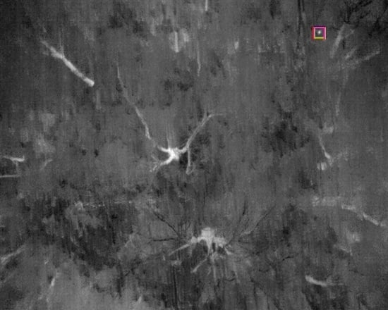
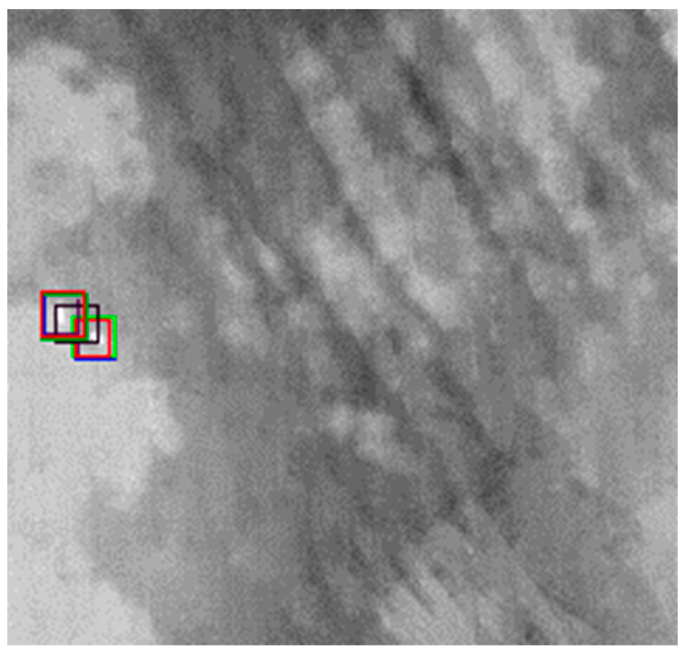
A range of detector ensembles were created from the individually trained copies of each model type and size. In the ensembles, following non-maximum suppression, detections were aggregated across component detectors, with overlapping detections grouped. A confidence score [0, 1] was calculated for each detection by the individual models, with 0 indicating no confidence and 1 indicating 100% confidence. The detection threshold was set at 0.5, so that initial detections with a confidence score below 50% were discarded, effectively dampening spurious detections. Same class detections were progressively merged based on the overlap of bounding boxes produced by the different detectors, with the Intersection-over-Union (IoU) threshold set at 0.8. This meant that detections from individual models within the ensemble with more than 80% overlap were progressively merged. The final detections output by the ensembles were based on the average of these merged detections and a final confidence score was given for each. This final confidence score is the sum of the confidence values for the individual grouped detections across the ensemble, divided by the total number of models in the ensemble. Figure 1, Figure 2 and Figure 3 show examples of frames where objects have been identified by different detectors within ensembles and then tracked according to the confidence value assigned to the detection.

Compared to the earlier method devised by [18] this approach has a number of benefits including avoiding the need to align consecutive frames to register detection results, which improves robustness in the presence of rapid camera motion, and offering a scalable solution where the complexity of an ensemble can be easily scaled by adding or removing detectors to meet diverse use cases.

The first group of ensembles comprised multiple copies of the same detector type and size. Individual copies were added one at a time, from highest to lowest individual AP, to allow the effect of each addition to be assessed. The next group of ensembles combined different numbers and sizes of all YOLO or all Detectron2 models exclusively. The AP values achieved by these ensembles informed the composition of the third and final group of ensembles, in which both types and sizes were mixed.

2.5. Ensemble Testing and Analysis

Four of the best performing ensembles were selected for testing on the unseen dataset. GPS coordinates associated with objects tracked by an ensemble indicated the position of the sensor on board the drone when the object was detected rather than the object itself. These locations were visualised in ArcGIS (v10.8) in order to identify instances where the same object was detected (duplicated) in multiple tracks. When visualised, duplicate tracks sometimes appear as a compact linear sequence of detections along the line of flight where continuous tracking has been interrupted by some occlusion. Duplicates can also occur in adjacent flight rows, where the same object is approached from opposite directions. We expect the number of duplicates to decrease as geolocation of target objects improves.

From analysis of the visualisation, the number of unique predictions was estimated for each ensemble. True positives were then confirmed by manual review against radio-collared koala locations, allowing precision (distinct from AP) and recall (probability of detection) values, and F1-scores to be calculated for each ensemble on the test dataset. An F1-score indicates the harmonic mean between precision and recall, which allows the overall performance to be evaluated in terms of the trade-off between the two important metrics, as shown in Equation (3):

F1 = 2 × [Precision × Recall]/[Precision + Recall]

(3)

3. Results

3.1. Model Training Summary

Thirty-five YOLO models were trained in total. All but one (extra-large) were trained on a desktop PC with a Nvidia RTX 3090 GPU, an Intel i7-11700K processor and 32 GB of RAM. Average training times for YOLO models trained on the desktop PC are shown in

Table 1. YOLO model training summary (desktop PC).

YOLO Size	Number Trained	Training Epochs	Batch Size	Average Training Time (Hours)
Tiny	10	250	32	3.40
Medium	10	250	32	6.64
Large	10	250	16	9.18
Extra-large	4	250	16	17.06

.

The additional extra-large YOLO was trained in a high-performance computing (HPC) environment, using Nvidia M40 GPUs and took 78.94 h to complete. Ten RetinaNet and 15 FR-CNN models were trained on the Detectron2 API. All but two were trained using the HPC environment. Training of the remaining two 50-layer RetinaNet models was 3.7 times faster on the desktop PC (average 2.93 h). Average training times for Detectron2 API models trained in the HPC environment are shown in

Table 2. Detectron2 API model training summary (HPC environment).

Detectron2 Model Type	Number Trained	Iterations	Average Training Time (Hours)
RetinaNet 50-layer	8	100,000	3.40
FR-CNN 50-layer	10	100,000	6.64
FR-CNN 101-layer	5	100,000	9.18

.

3.2. Average Precision of Individual Models

Tables showing AP achieved by all individual and ensemble detectors are provided in Appendix A. Individual YOLO models of all sizes consistently achieved higher AP than any Detectron2 type or size (

Table A1. AP values of all individually trained copies of each detector type and size, ranked highest to lowest.

	YOLO Tiny	YOLO Medium	YOLO Large	YOLO X-Large	RetinaNet-50	FR-CNN-50	FR-CNN-101
Copy 1	0.9568	0.9731	0.9800	0.9698	0.8421	0.8532	0.8436
Copy 2	0.9556	0.9718	0.9786	0.9676	0.8306	0.8443	0.8703
Copy 3	0.9551	0.9711	0.9783	0.9456	0.8304	0.8438	0.8679
Copy 4	0.9538	0.9700	0.9780	0.9452	0.8278	0.8309	0.8679
Copy 5	0.9498	0.9668	0.9760	0.9146	0.8247	0.8286	0.8504
Copy 6	0.9464	0.9663	0.9748		0.8144	0.8268
Copy 7	0.9463	0.9629	0.9725		0.8117	0.8215
Copy 8	0.9410	0.9597	0.9724		0.8029	0.8145
Copy 9	0.9390	0.9556	0.9692		0.7862	0.8110
Copy 10	0.9340	0.9307	0.9542		0.7783	0.8085
Mean AP ± SD	0.9478 ± 0.0078	0.9628 ± 0.0126	0.9734 ± 0.0075	0.9486 ± 0.0223	0.8149 ± 0.0206	0.8283 ± 0.0151	0.8600 ± 0.0122

). Of the individual copies, a large YOLO achieved the highest AP of all models (0.9800) and large YOLOs performed best overall (mean AP ± SD = 0.9734 ± 0.0078). All YOLO models achieved AP > 90% (minimum YOLO AP = 0.9146 by an extra-large) whereas AP for Detectron2 models ranged between 0.7783 (50-layer RetinaNet) and 0.8532 (50-layer FR-CNN). The greatest variation in AP occurred in extra-large YOLO models (SD = 0.0223) followed by 50-layer RetinaNet (SD = 0.0206). Large YOLO and tiny YOLO models showed the least variation (SD = 0.0075; 0.0078).

3.3. Average Precision of Single Type and Size Ensembles

Single-size YOLO ensembles outperformed single-type-and-size Detectron2 ensembles, with the highest AP value exceeding 97% for every size of YOLO (

Table A2. AP values of ensembles built from individually trained copies of each detector type and size.

	YOLO Tiny	YOLO Medium	YOLO Large	YOLO X-Large	RetinaNet-50	FR-CNN-50	FR-CNN-101
1 copy	0.9568	0.9731	0.9800	0.9698	0.8421	0.8532	0.8703
2 copies	0.9476	0.9754	0.9805	0.9716	0.8484	0.8449	0.8728
3 copies	0.9555	0.9784	0.9820	0.9720	0.8580	0.8500	0.8784
4 copies	0.9621	0.9784	0.9820	0.9773	0.8652	0.8506	0.8879
5 copies	0.9662	0.9782	0.9834	0.9738	0.8699	0.8487	0.8861
6 copies	0.9698	0.9782	0.9834		0.8696	0.8487
7 copies	0.9712	0.9782	0.9834		0.8692	0.8473
8 copies	0.9711	0.9813	0.9818		0.8671	0.8507
9 copies	0.9724	0.9796	0.9831		0.8675	0.8524
10 copies	0.9723	0.9814	0.9849		0.8652	0.8520
Rank	4	2	1	3	6	7	5

). The best AP was achieved by an ensemble of 10 × large YOLOs (0.9849) closely followed by 10 × medium YOLOs (0.9814). These values were well above anything achieved by Detectron2 same-type-and-size ensembles, for which maximum AP ranged between 0.8524 (9 × 50-layer FR-CNNs) and 0.8879 (4 × 101-layer FR-CNNs). Interestingly, AP did not always improve as additional copies were added to the ensembles, for example, the 5-copy RetinaNet ensemble outperformed all larger RetinaNet ensembles.

3.4. Composition and Average Precision of Mixed Size All-YOLO Ensembles

Ensembles comprising only YOLO models, of mixed numbers and sizes, were built and tested in the order shown in

Table A3. Composition and AP values of ensembles comprising only YOLO detectors.

All YOLO	YOLO Tiny	YOLO Med	YOLO Large	YOLO X-Large	Time (Mins)	AP
1	×1	×1	×1	×1	3	0.9857
2	-	×1	×1	×1	3	0.9859
3	×5	×5	×5	×5	14	0.9878
4	×5	×5	×5	-	8	0.9880
5	-	×5	×5	×5	12	0.9864
6	-	-	×5	×5	10	0.9858
7	-	×5	×5	-	6	0.9884
8	-	×5	×5	×1	7	0.9884
9	-	×10	×10	-	11	0.9865
10	-	×10	×10	×1	13	0.9865
11	-	-	×10	×5	14	0.9840

. The initial combination of one YOLO of each size performed better than all single-type-and-size ensembles (0.9857), and removing the tiny YOLO achieved a further slight increase (0.9859). Both these combinations had the shortest run times of any ensembles (3 min). Five of each size lifted AP again (0.9878), but run time was almost 5× longer (14 min). Combining ten of any size also increased run time but without the additional benefit in performance. A combination of only large and extra-large YOLOs produced the lowest AP and was equal slowest (0.9840; 14 min). The best performer (0.9884) and second-fastest (6 min) was built from five medium and five large YOLOs with no other sizes.

3.5. Composition and Average Precision of Mixed All-Detectron2 Ensembles

Ensembles comprising only Detectron2 models, of mixed types, numbers and sizes, were built and tested in the order shown in

Table A4. Composition and AP values of ensembles comprising only Detctron2 API detectors.

All Det2	Ret-50	FRCNN-50	FRCNN-101	Time (Mins)	AP
1	×1	×1	×1	8	0.8776
2	×1	×1	-	5	0.8743
3	×1	-	×1	6	0.8640
4	-	×1	×1	6	0.8916
5	×5	×5	-	24	0.8808
6	×5	-	×1	14	0.8738
7	×1	-	×5	20	0.8811
8	×5	-	×5	27	0.8833
9	×5	×5	×1	27	0.8823
10	×10	×1	×1	27	0.8754
11	-	×5	×5	30	0.9003
12	-	×2	×2	12	0.9093
13	×1	×2	×2	14	0.8875

. The initial combination of one of each type and size (0.8776) performed well below the lowest all-YOLO ensemble (0.9840). Performance decreased when either of the FR-CNN sizes was removed (0.8743; 0.8640) but increased notably when the single 50-layer RetinaNet model was omitted (0.8916). In fact, all the ensembles with RetinaNet models achieved lower AP. Run time for single copy Detectron2 combinations was within the mid-range of the YOLO ensembles (6–8 min) but ensembles with five or more copies were significantly slower (20+ min). The best performing all-Detectron2 ensemble combined two copies of each FR-CNN size (0.9093) and decreased processing time to 12 min.

3.6. Composition and Average Precision of Mixed Type and Size Ensembles

Ensembles comprising models of any type and size were built and tested in the order shown in

Table A5. Composition and AP values of mixed ensembles.

Mix	YOLO Tiny	YOLO Med	YOLO Large	YOLO X-Large	Ret-50	FRCNN-50	FRCNN-101	Time (Mins)	AP
1	×1	×1	×1	×1	×1	×1	×1	11	0.9875
2	×1	×1	×1	-	×1	×1	×1	9	0.9838
3	×1	×1	×1	×1	-	×1	×1	8	0.9891
4	×1	×1	×1	-	-	×1	×1	8	0.9879
5	-	×1	×1	-	-	×1	×1	8	0.9854
6	-	×2	×2	-	-	×2	×2	15	0.9857
7	-	×5	×5	-	-	×5	×5	34	0.9845
8	-	×5	×5	-	-	×2	×2	17	0.9881
9	-	×5	×5	-	×1	×2	×2	19	0.9883
10	×1	×5	×5	×1	×1	×2	×2	21	0.9887
11	×1	×2	×2	×1	-	×2	×2	18	0.9864

. All mixed type ensembles achieved AP above 98%. An initial ensemble combining the best performing of each model provided a baseline. The AP was slightly below the best performing all-YOLO ensemble (0.9875 vs. 0.9884), with run time of 11 min. The ensemble with one of each type-size, excluding RetinaNet, achieved a new highest AP (0.9891) with relatively low run time (8 min). A combination of 5 × medium and large YOLOs, 2 × each FR-CNN, and 1 × all other models achieved the second highest AP (0.9887) but run time increased to 21 min.

3.7. Selection of Best Performing Ensembles

The ensembles in

Table 3. Composition and AP values of best performing ensembles overall.

Ensemble	YOLO Tiny	YOLO Med	YOLO Large	YOLO X-Large	Ret-50	FRCNN-50	FRCNN-101	Time (Mins)	AP
All Det2 12	-	-	-	-	-	×2	×2	12	0.9093
10× tiny YOLO	×10	-	-	-	-	-	-	4	0.9723
9× tiny YOLO	×9	-	-	-	-	-	-	4	0.9724
All YOLO 8	-	×5	×5	×1	-	-	-	7	0.9884
All YOLO 7	-	×5	×5	-	-	-	-	6	0.9884
Mix 10	×1	×5	×5	×1	×1	×2	×2	21	0.9887
Mix 3	×1	×1	×1	×1	-	×1	×1	8	0.9891

showed the highest potential overall for detecting small-bodied wildlife from low-altitude data, while keeping processing time generally low. The larger and more complex ‘All Det2 11’ achieved very similar AP to ‘All Det2 12’ but used considerably more time for processing so is not included. While ‘Mix 10’ had a substantially higher run time than ‘Mix 3’, it is still considered a good option for further testing to determine whether there is any benefit to be gained from the greater variety in its component models. Large tiny YOLO ensembles, which are very lightweight, are included because of their potential for use in on-board processing.

3.8. Ensemble Testing and Analysis Results

The previous section used widely used object detection metrics to assess the accuracy of component models and ensemble combinations on validation data, where detections in each frame were considered independently to obtain overall measures. An alternative approach was required to assess the performance of the selected ensembles when tested on unseen data. Our ensemble approach associates detections based on their geographical position, then uses the expected sensor (drone) motion to group detections that occur in consecutive frames into “tracks”. As this produces correspondence between frames, detections can no longer be considered independent and so the following analysis is conducted at the “track” level.

Four ensembles were selected to run over the testing dataset—the best performing (highest AP) all-YOLO, all-Detectron2 and mixed-type combination as well as the second best mixed-type, as this was the largest and most diverse of the group. Processing times and output metrics are shown in

Table 4. Processing metrics for selected ensemble tests.

Ensemble	Processing Time	# Tracked Objects	# Tracked Frames	Average Frames/Tracked Object
All YOLO 7	1:57	48	303	6.3
All Det2 12	4:04	460	3594	7.8
Mix 3	2:56	58	429	7.4
Mix 10	6:58	30	232	7.7

.

The all-YOLO ensemble processed image frames much faster than the other ensembles, and the objects it detected were, on average, tracked over fewer frames. The ‘mix 10’ ensemble produced the lowest number of tracks and frames but was significantly slower than others. The all-Detectron2 ensemble produced an order of magnitude more tracks and frames than all others, which has time and resource implications where manual verification is required.

Ensemble performance was then evaluated and compared with the results of Ref. [18]. One koala was excluded from this study at this point as it was technically beyond our survey boundary, giving a total of 17 ground-truths. This koala was included by Ref. [18] and the removal elevated detection probability (recall) of that survey to 100%. As the data used to train our component models encompassed a broader range of spatial and temporal settings than the training data used by Ref. [18], it was anticipated this study was unlikely to perform as well. Nonetheless, evaluation against Ref. [18] provides a fair measure of robustness of the ensemble approach. Prior to calculating the recall, precision and F-1 score of each ensemble, duplicate tracks were identified so that the number of unique predictions could be estimated. The performance metrics are summarised in

Table 5. Performance metrics for selected ensembles compared to Ref. [18].

Ground Truths = 17	True Positives	Detection Probability (Recall)	Total Tracked Objects	Unique Tracks	Precision	F1-Score
[18]	17	100%	-	-	69%	0.8166
All Det2 12	17	100%	460	No further analysis undertaken
All YOLO 7	12	71%	48	26	46%	0.5581
Mix 3	12	71%	58	21	57%	0.6316
Mix 10	12	71%	30	16	75%	0.7273

.

4. Discussion

While technologies such as drones and thermal imaging are enabling advances in environmental surveying, ecologists are struggling to process the large datasets generated with these tools. This is especially true for small and cryptic wildlife which do not feature strongly in the literature, with the majority of automated detection research to date focussed on large-bodied mammals or birds that are easily discernible from relatively homogeneous backgrounds [20]. The study by [18] was the first to successfully apply automated detection to a small-bodied arboreal mammal from thermal imagery. While at the time the method was innovative for cryptic wildlife detection, deep learning has continued to evolve rapidly, and the algorithms used in that study are no longer cutting edge. While ensembles have been used in other domains, this is the first time that ensembles have been used in ecology for the detection of threatened species using drone-derived data. The deep learning ensembles provide much greater computational power, deriving valuable synergies from running suites of high-performance algorithms simultaneously. Our systematic study has devised a quantitative method for evaluating the combinations that achieve high precision and recall in small-bodied, arboreal wildlife detection and has demonstrated the utility of the approach. The results are strong in the broader computer vision context, with one article published in 2021 [28] highlighting the lack of focus on small object detection and summarising mean AP values achieved from low-altitude aerial datasets as between 19% and 41%. Our results are particularly promising given the benefit that can be derived from further fine-tuning iterations which can prepare the ensembles for specific contexts and require only minimal datasets for training. While we did not expect our study to match the results of [18] because our training data encompassed broader spatial and temporal settings, the ensembles nonetheless tested well with minimal training.

The shift to an ensemble approach offers a number of advantages that increase detector robustness. The ensembles are built from state-of-the-art models which perform better when detecting small targets, thus reducing the need to register frames for accumulating detections over time. It is also advantageous to use a larger number of simpler, faster models to estimate uncertainty with respect to detection. The approach can also be scaled for specific platforms without changing the underlying system, so that smaller and simpler ensembles can be employed when circumstances require, for example in an on-board setting, and larger ensembles can be used when more hardware is available.

The best performing ensemble contained the greatest diversity of component models, demonstrating the benefit of ensemble learning which exploits the various architectural strengths and minimises the weaknesses [29,30,31,32,33]. In the validation phase, YOLO models consistently featured in high-performing ensembles, suggesting that their inclusion may be valuable when constructing ensembles for processing low-altitude imagery. The medium YOLO, in particular, appeared to be a valuable contributor to ensemble performance. While not subject to final testing, the relatively strong AP achieved by the 9× and 10× tiny YOLO ensembles in validation recommends them for innovations such as on-board processing, as they are very lightweight in nature.

Perhaps surprisingly, the inclusion of RetinaNet models did not appear to be advantageous, and RetinaNet models were present in some of the lowest AP ensembles in the validation stage. The entire suite of ‘All Det2’ ensembles achieved lower AP than any of the ensembles containing YOLO components; however, the ten ‘All Det2’ ensembles that included RetinaNet models (with copies ranging in number between 1 and 10) were the lowest scoring of all. It is perhaps contradictory then that ‘Mix 10’, which performed best in testing, was the only tested ensemble with a RetinaNet component. ‘Mix 10’ however was a large and diverse ensemble, and it is possible that the computational power of the other components overcame any impediment the RetinaNet may have presented. It may be useful to test the same combination with the single RetinaNet excluded.

As well as performance accuracy, the evaluation of object detection models should encompass computational complexity and inference (processing) time [28]. In this study, ensembles which included YOLO detectors had lower processing times which is to be expected given YOLO’s single step architecture. The longest run times occurred with ensembles containing more than one copy of an F-RCNN models, both 50- and 101-layer, which is again unsurprising given their region-based approach and more computationally complex backbone. Surprisingly, however, the inclusion of single-step RetinaNet components did not correspond with shorter run times. As drone-acquired datasets are generally large compared to typical photographic imagery, processing time is likely to be an important consideration in the context of small-bodied wildlife detection. The optimal ensemble will need to provide a judicious balance between inference time and accuracy for a given monitoring activity, but the inclusion of at least some YOLO components is strongly indicated.

The greatest impediment to higher precision in our ensemble approach was the number of false positive objects that were tracked. This was particularly the case for the ‘All Det2 12’ ensemble, which produced 100% recall but a challenging number of tracked objects. To reduce false positives, future studies could apply a threshold to discard objects that are not tracked over some minimum number of frames. It is also possible, however, that uncollared koalas may have been present in the survey area so that detections that appear spurious could in fact have been correct.

In addition to the novel application of ensemble learning for automated detection of small-bodied wildlife from low-altitude drone surveys, an important feature of this study is the quantitative approach that has been devised to measure and compare model performance. Explicit rates of precision are rarely reported in ecological studies where drone surveys have been combined with automated wildlife detection [20]. Deep learning ensembles in this study have achieved very high AP when tested on validation data. Our training data in this study intentionally encompassed a broader range of environments and habitats than [18], an approach designed to ensure greater robustness across more diverse settings, compared to [18] which was specifically trained for detections at Petrie. As a result, it was expected that performance would decrease when used on unseen testing data, where contextual semantic (background) information differed from that of the training data. However, precision can be reasonably expected to increase over time as continuous fine-tuning is undertaken based on errors identified in each new setting. Additionally, approximately 50% of the images in our validation dataset contained a koala which is a far greater concentration than the proportion found in one complete survey such as our testing dataset.

5. Conclusions

We have demonstrated the suitability and high potential of deep learning ensembles and provided a quantitative approach to optimising ensemble composition. The approach not only offers much-needed efficiencies in data processing but also significantly enhances computational power and an ability currently lacking to scale up or down in response to environmental and computational constraints or demands. Future exploration of this high-potential approach should include improved geolocation of tracked objects and the use of thresholds to reduce false positive detections.

References

1. Callaghan, C.T.; Poore, A.G.B.; Major, R.E.; Rowley, J.J.L.; Cornwell, W.K. Optimizing future biodiversity sampling by citizen scientists. Proc. R. Soc. B Biol. Sci. 2019, 286, 20191487. [Google Scholar] [CrossRef] [PubMed]
2. Corcoran, E.; Denman, S.; Hamilton, G. New technologies in the mix: Assessing N-mixture models for abundance estimation using automated detection data from drone surveys. Ecol. Evol. 2020, 10, 8176–8185. [Google Scholar] [CrossRef] [PubMed]
3. Gentle, M.; Finch, N.; Speed, J.; Pople, A. A comparison of unmanned aerial vehicles (drones) and manned helicopters for monitoring macropod populations. Wildl. Res. 2018, 45, 586–594. [Google Scholar] [CrossRef]
4. Lethbridge, M.; Stead, M.; Wells, C. Estimating kangaroo density by aerial survey: A comparison of thermal cameras with human observers. Wildl. Res. 2019, 46, 639–648. [Google Scholar] [CrossRef]
5. Longmore, S.N.; Collins, R.P.; Pfeifer, S.; Fox, S.E.; Mulero-Pázmány, M.; Bezombes, F.; Goodwin, A.; De Juan Ovelar, M.; Knapen, J.H.; Wich, S.A. Adapting astronomical source detection software to help detect animals in thermal images obtained by unmanned aerial systems. Int. J. Remote Sens. 2017, 38, 2623–2638. [Google Scholar] [CrossRef]
6. Tanwar, K.S.; Sadhu, A.; Jhala, Y.V. Camera trap placement for evaluating species richness, abundance, and activity. Sci. Rep. 2021, 11, 23050. [Google Scholar] [CrossRef]
7. Witczuk, J.; Pagacz, S.; Zmarz, A.; Cypel, M. Exploring the feasibility of unmanned aerial vehicles and thermal imaging for ungulate surveys in forests—Preliminary results. Int. J. Remote Sens. 2018, 39, 5504–5521. [Google Scholar] [CrossRef]
8. Hong, S.J.; Han, Y.; Kim, S.Y.; Lee, A.Y.; Kim, G. Application of deep-learning methods to bird detection using unmanned aerial vehicle imagery. Sensors 2019, 19, 1651. [Google Scholar] [CrossRef] [Green Version]
9. Leigh, C.; Heron, G.; Wilson, E.; Gregory, T.; Clifford, S.; Holloway, J.; McBain, M.; Gonzalez, F.; McGree, J.; Brown, R.; et al. Using virtual reality and thermal imagery to improve statistical modelling of vulnerable and protected species. PLoS ONE 2019, 14, e0217809. [Google Scholar] [CrossRef] [Green Version]
10. Nazir, S.; Kaleem, M. Advances in image acquisition and processing technologies transforming animal ecological studies. Ecol. Inform. 2021, 61, 101212. [Google Scholar] [CrossRef]
11. Prosekov, A.; Kuznetsov, A.; Rada, A.; Ivanova, S. Methods for monitoring large terrestrial animals in the wild. Forests 2020, 11, 808. [Google Scholar] [CrossRef]
12. Seymour, A.C.; Dale, J.; Hammill, M.; Halpin, P.N.; Johnston, D.W. Automated detection and enumeration of marine wildlife using unmanned aircraft systems (UAS) and thermal imagery. Sci. Rep. 2017, 7, 45127. [Google Scholar] [CrossRef] [PubMed] [Green Version]
13. Beaver, J.T.; Baldwin, R.W.; Messinger, M.; Newbolt, C.H.; Ditchkoff, S.S.; Silman, M.R. Evaluating the Use of Drones Equipped with Thermal Sensors as an Effective Method for Estimating Wildlife. Wildl. Soc. B 2020, 44, 434–443. [Google Scholar] [CrossRef]
14. Chrétien, L.P.; Théau, J.; Ménard, P. Visible and thermal infrared remote sensing for the detection of white-tailed deer using an unmanned aerial system. Wildl. Soc. B 2016, 40, 181–191. [Google Scholar] [CrossRef]
15. Goodenough, A.E.; Carpenter, W.S.; MacTavish, L.; Theron, C.; Delbridge, M.; Hart, A.G. Identification of African antelope species: Using thermographic videos to test the efficacy of real-time thermography. Afr. J. Ecol. 2018, 56, 898–907. [Google Scholar] [CrossRef]
16. Hamilton, G.; Corcoran, E.; Denman, S.; Hennekam, M.E.; Koh, L.P. When you can’t see the koalas for the trees: Using drones and machine learning in complex environments. Biol. Conserv. 2020, 247, 108598. [Google Scholar] [CrossRef]
17. Chrétien, L.P.; Théau, J.; Ménard, P. Wildlife multispecies remote sensing using visible and thermal infrared imagery acquired from an unmanned aerial vehicle (UAV). Int. Arch. Photogramm. Remote Sens. 2015, XL-1/W4, 241–248. [Google Scholar] [CrossRef] [Green Version]
18. Corcoran, E.; Denman, S.; Hanger, J.; Wilson, B.; Hamilton, G. Automated detection of koalas using low-level aerial surveillance and machine learning. Sci. Rep. 2019, 9, 3208. [Google Scholar] [CrossRef] [Green Version]
19. Conn, P.B.; Ver Hoef, J.M.; McClintock, B.T.; Moreland, E.E.; London, J.M.; Cameron, M.F.; Dahle, S.P.; Boveng, P.L. Estimating multispecies abundance using automated detection systems: Ice-associated seals in the Bering Sea. Methods Ecol. Evol. 2014, 5, 1280–1293. [Google Scholar] [CrossRef]
20. Corcoran, E.; Winsen, M.; Sudholz, A.; Hamilton, G. Automated detection of wildlife using drones: Synthesis, opportunities and constraints. Methods Ecol. Evol. 2021, 12, 1103–1114. [Google Scholar] [CrossRef]
21. Pimm, S.L.; Alibhai, S.; Bergl, R.; Dehgan, A.; Giri, C.; Jewell, Z.; Joppa, L.; Kays, R.; Loarie, S. Emerging Technologies to Conserve Biodiversity. Trends Ecol. Evol. 2015, 30, 685–696. [Google Scholar] [CrossRef]
22. Kellenberger, B.; Marcos, D.; Tuia, D. Detecting mammals in UAV images: Best practices to address a substantially imbalanced dataset with deep learning. Remote Sens. Environ. 2018, 216, 139–153. [Google Scholar] [CrossRef] [Green Version]
23. Chabot, D.; Stapleton, S.; Francis, C.M. Using Web images to train a deep neural network to detect sparsely distributed wildlife in large volumes of remotely sensed imagery: A case study of polar bears on sea ice. Ecol. Inform. 2022, 68, 101547. [Google Scholar] [CrossRef]
24. Kellenberger, B.; Veen, T.; Folmer, E.; Tuia, D. 21 000 birds in 4.5 h: Efficient large-scale seabird detection with machine learning. Remote Sens. Ecol. Conserv. 2021, 7, 445–460. [Google Scholar] [CrossRef]
25. Duporge, I.; Isupova, O.; Reece, S.; Macdonald, D.W.; Wang, T. Using very-high-resolution satellite imagery and deep learning to detect and count African elephants in heterogeneous landscapes. Remote Sens. Ecol. Conserv. 2021, 7, 369–381. [Google Scholar] [CrossRef]
26. Kays, R.; Sheppard, J.; McLean, K.; Welch, C.; Paunescu, C.; Wang, V.; Kravit, G.; Crofoot, M. Hot monkey, cold reality: Surveying rainforest canopy mammals using drone-mounted thermal infrared sensors. Int. J. Remote Sens. 2019, 40, 407–419. [Google Scholar] [CrossRef]
27. Menikdiwela, M.; Nguyen, C.; Li, H.; Shaw, M. CNN-based small object detection and visualization with feature activation mapping. In Proceedings of the 2017 International Conference on Image and Vision Computing New Zealand, Christchurch, New Zealand, 4–6 December 2017. [Google Scholar] [CrossRef]
28. Mittal, P.; Singh, R.; Sharma, A. Deep learning-based object detection in low-altitude UAV datasets: A survey. Image Vision Comput. 2020, 104, 104046. [Google Scholar] [CrossRef]
29. Dong, X.; Yu, Z.; Cao, W.; Shi, Y.; Ma, Q. A survey on ensemble learning. Front. Comput. Sci. 2020, 14, 241–258. [Google Scholar] [CrossRef]
30. Gomez-Donoso, F.; Escalona, F.; Pérez-Esteve, F.; Cazorla, M. Accurate multilevel classification for wildlife images. Comput. Intel. Neurosc. 2021, 2021, 6690590. [Google Scholar] [CrossRef]
31. Kumar, A.; Kim, J.; Lyndon, D.; Fulham, M.; Feng, D. An Ensemble of Fine-Tuned Convolutional Neural Networks for Medical Image Classification. IEEE J. Biomed. Health 2017, 21, 7769199. [Google Scholar] [CrossRef] [Green Version]
32. Morovati, M.; Karami, P.; Amjas, F.B. Accessing habitat suitability and connectivity for the westernmost population of Asian black bear (Ursus thibetanus gedrosianus, Blanford, 1877) based on climate changes scenarios in Iran. PLoS ONE 2020, 15, e0242432. [Google Scholar] [CrossRef] [PubMed]
33. Yang, D.Q.; Tan, K.; Huang, Z.P.; Li, X.W.; Chen, B.H.; Ren, G.P.; Xiao, W. An automatic method for removing empty camera trap images using ensemble learning. Ecol. Evol. 2021, 11, 7591–7601. [Google Scholar] [CrossRef] [PubMed]
34. Ying, X. Ensemble Learning; University of Georgia: Athens, GA, USA, 2014; Available online: https://www.researchgate.net/publication/262369664_Ensemble_Learning (accessed on 14 December 2021).
35. Carter, S.; van Rees, C.B.; Hand, B.K.; Muhlfeld, C.C.; Luikart, G.; Kimball, J.S. Testing a generalizable machine learning workflow for aquatic invasive species on rainbow trout (Oncorhynchus mykiss) in Northwest Montana. Front. Big Data 2021, 4, 734990. [Google Scholar] [CrossRef] [PubMed]
36. Giese, L.; Melzheimer, J.; Bockmühl, D.; Wasiolka, B.; Rast, W.; Berger, A.; Wachter, B. Using machine learning for remote behaviour classification—Verifying acceleration data to infer feeding events in free-ranging cheetahs. Sensors 2021, 21, 5426. [Google Scholar] [CrossRef] [PubMed]
37. Yu, J.; Su, H.; Liu, J.; Yang, Z.; Zhang, Z.; Zhu, Y.; Yang, L.; Jiao, B. A strong baseline for tiger re-ID and its bag of tricks. In Proceedings of the 2019 IEEE/CVF International Conference on Computer Vision Workshop (ICCVW), Seoul, Korea, 27–28 October 2019; pp. 302–309. [Google Scholar]
38. Padilla, R.; Netto, S.L.; da Silva, E.A.B. A survey on performance metrics for object-detection algorithms. In Proceedings of the 2020 International Conference on Systems, Signals and Image Processing, Rio de Janeiro, Brazil, 1–3 July 2020; Available online: https://ieeexplore.ieee.org/document/9145130 (accessed on 24 December 2021).
39. Oksuz, K.; Cam, B.C.; Akbas, E.; Kalkan, S. Localization recall precision (LRP): A new performance metric for object detection. In Computer Vision—ECCV 2018, Lecture Notes in Computer Science; Ferrari, V., Hebert, M., Sminchisescu, C., Weiss, Y., Eds.; Springer: Cham, Switzerland, 2018; Volume 11211. [Google Scholar] [CrossRef] [Green Version]
40. Saunders, B.; Sim, J.; Kingstone, T.; Baker, S.; Waterfield, J.; Bartlam, B.; Burroughs, H.; Jinks, C. Saturation in qualitative research: Exploring its conceptualization and operationalization. Qual. Quant. 2018, 52, 1893–1907. [Google Scholar] [CrossRef] [PubMed]
Figure 1. Single frame showing two objects, each with overlapping bounding boxes, that have been recognised by different component detectors within an ensemble. The different coloured boxes represent different component detectors. The strength of the outline represents the confidence value assigned to each detection.
Remotesensing 14 02432 g001
Figure 2. Two objects identified in a single frame as potential koalas. The object at the left of the frame is being tracked by multiple component detectors with relatively high confidence, while the object at the right is being tracked by just one detector with lower confidence. If confidence falls below the threshold level, tracking of the object will cease.
Remotesensing 14 02432 g002
Figure 3. This frame shows the value of the ensemble’s ability to incorporate spatial dependencies. As these objects are tracked across frames, contextual clues will lower the confidence values of these tracks which will result in these objects, which are actually tree limbs, being discarded as possible koala detections.
Remotesensing 14 02432 g003