
Characterizing the Patterns and Trends of Urban Growth in Saudi Arabia’s 13 Capital Cities Using a Landsat Time Series


Abstract
:1. Introduction
2. Study Area and Methods
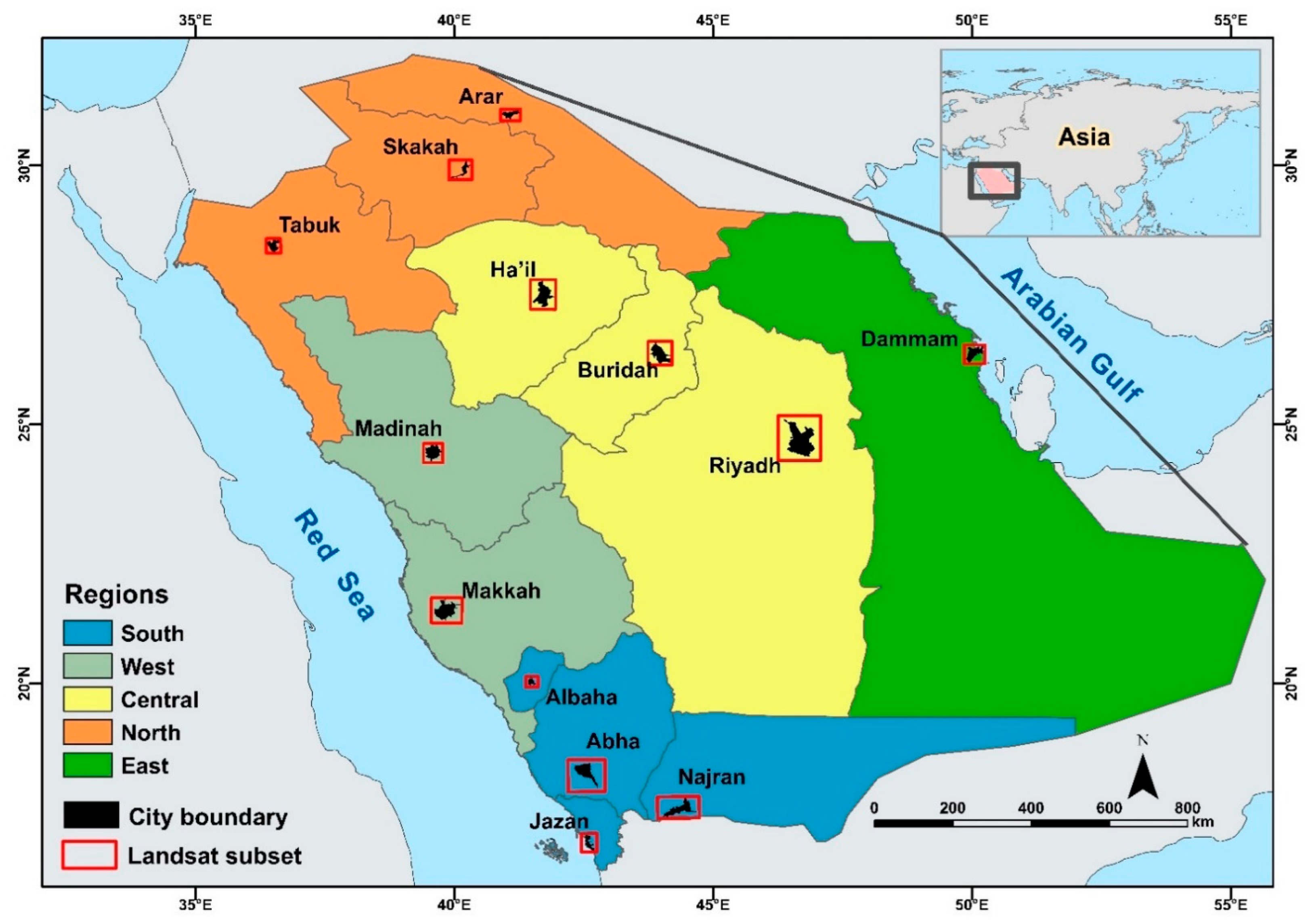
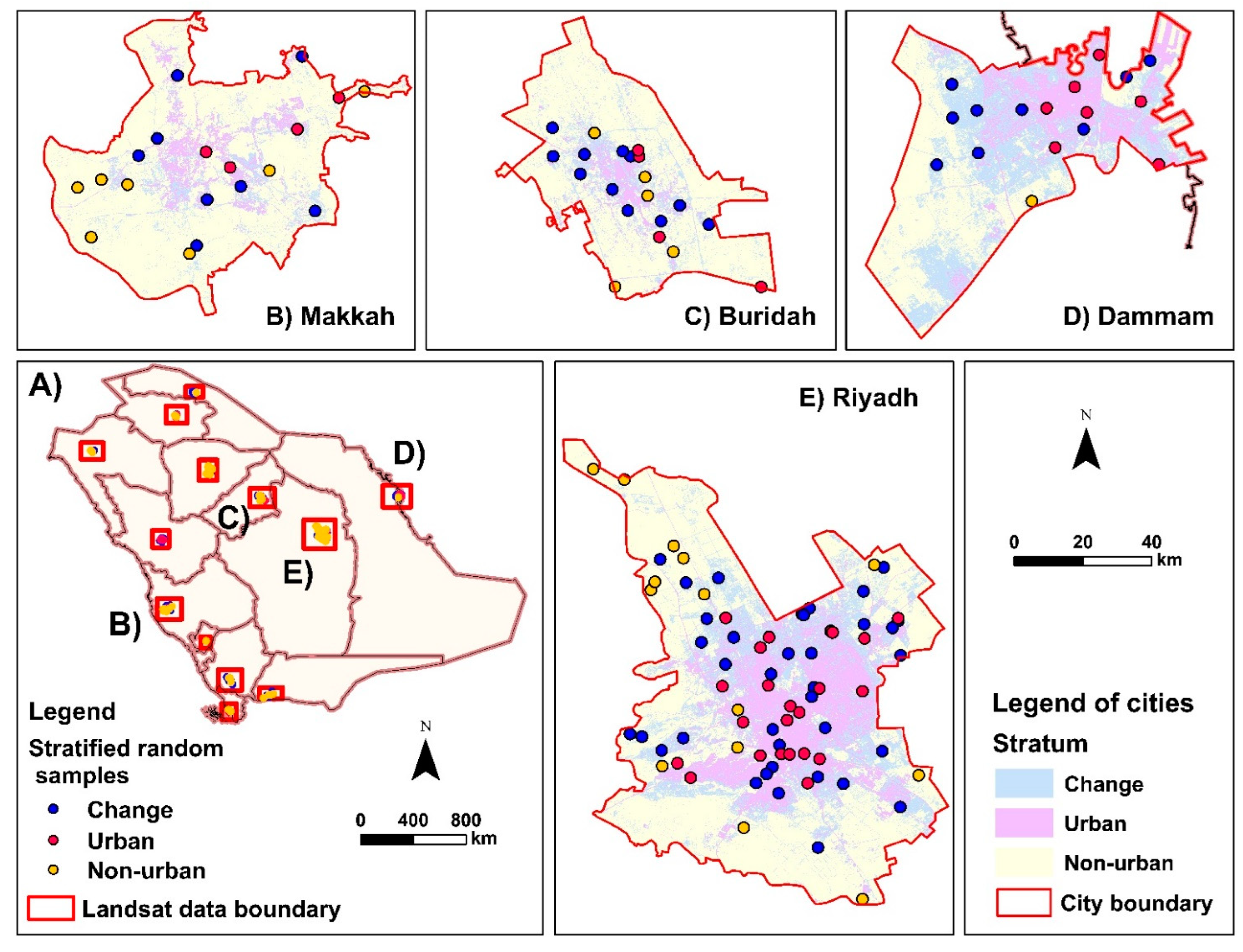
2.1. Study Area
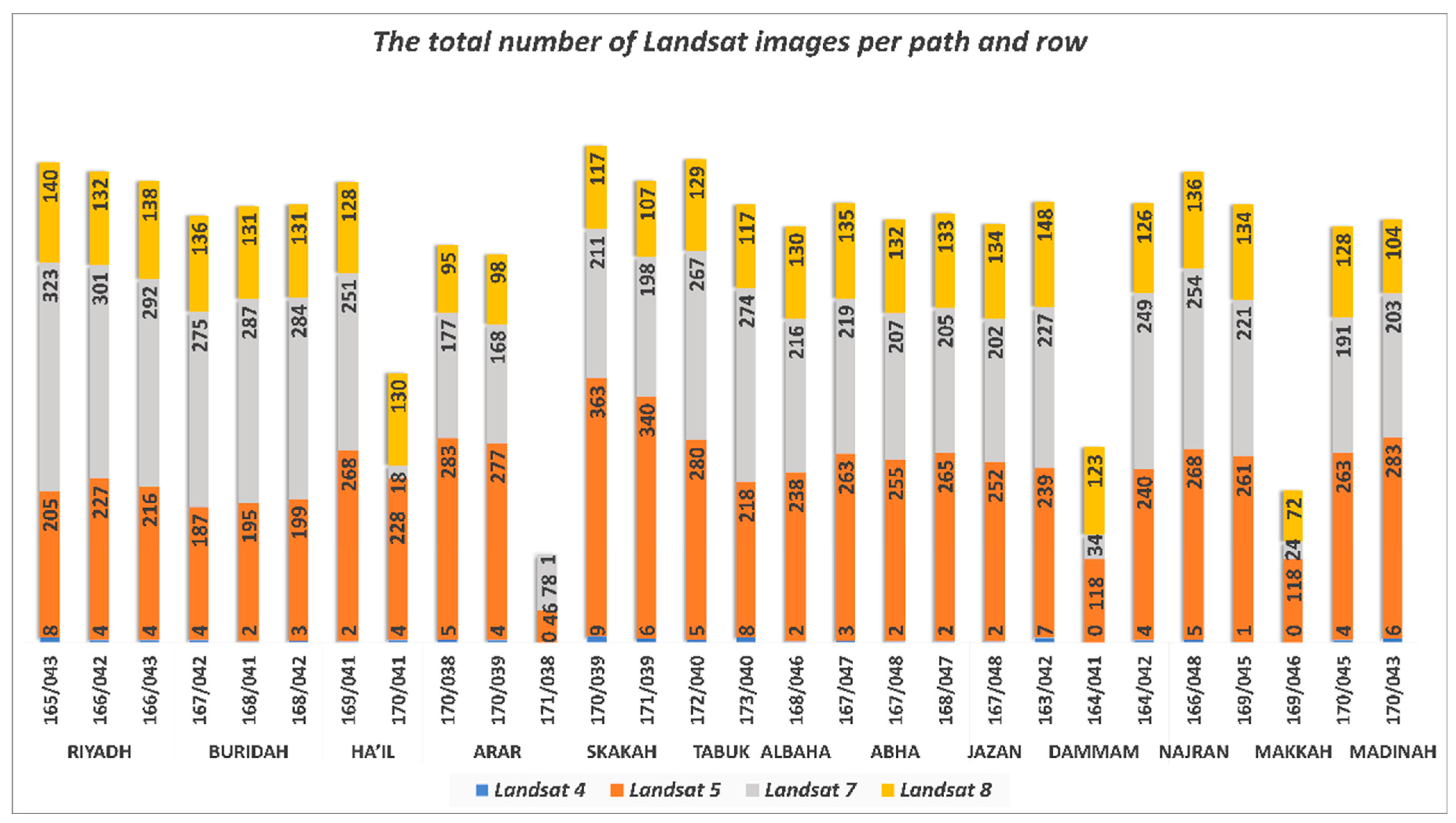
2.2. Landsat Data
3. Data Processing
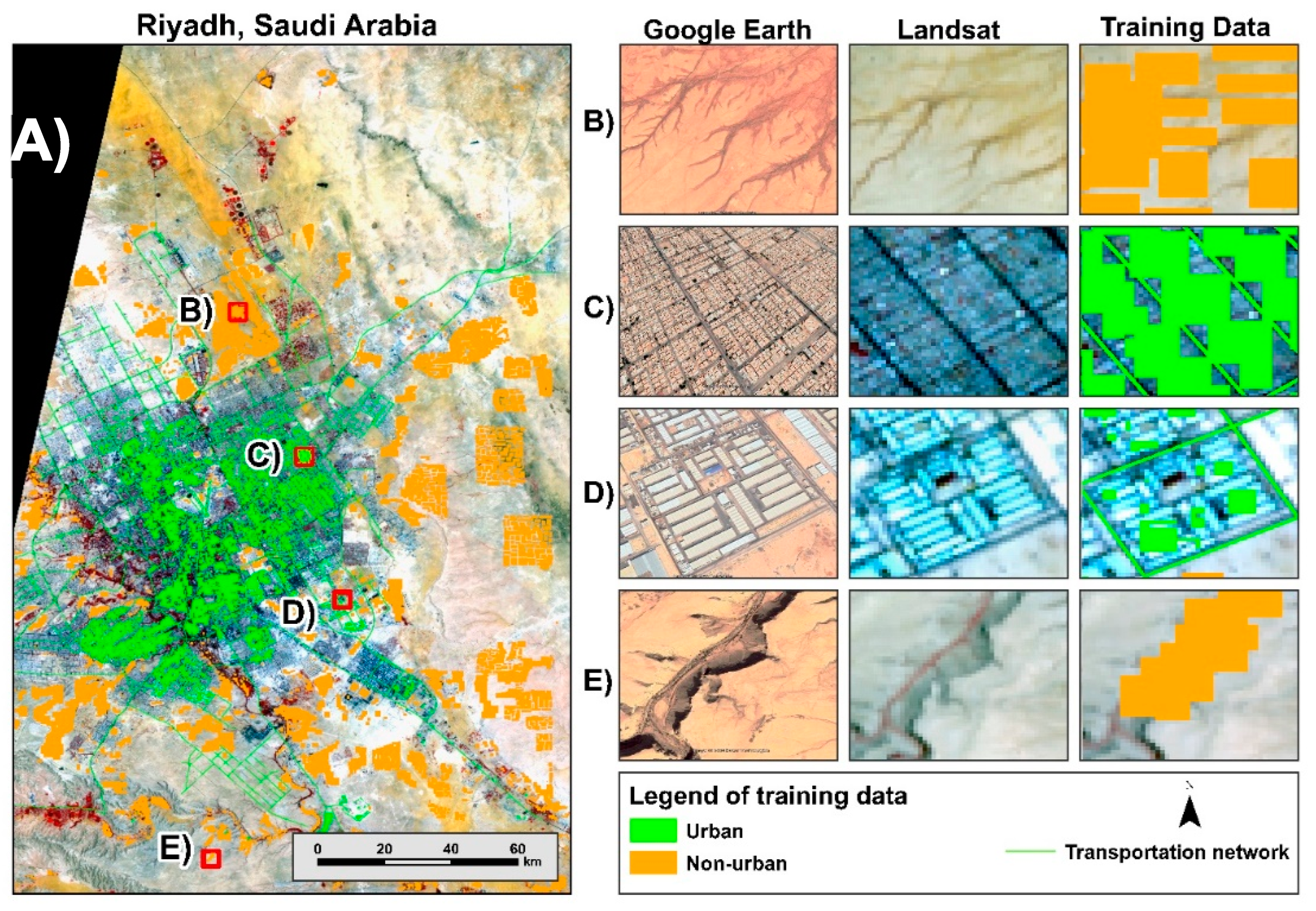
3.1. Training Data
3.2. CCDC Algorithm for Continuous Urban Classification
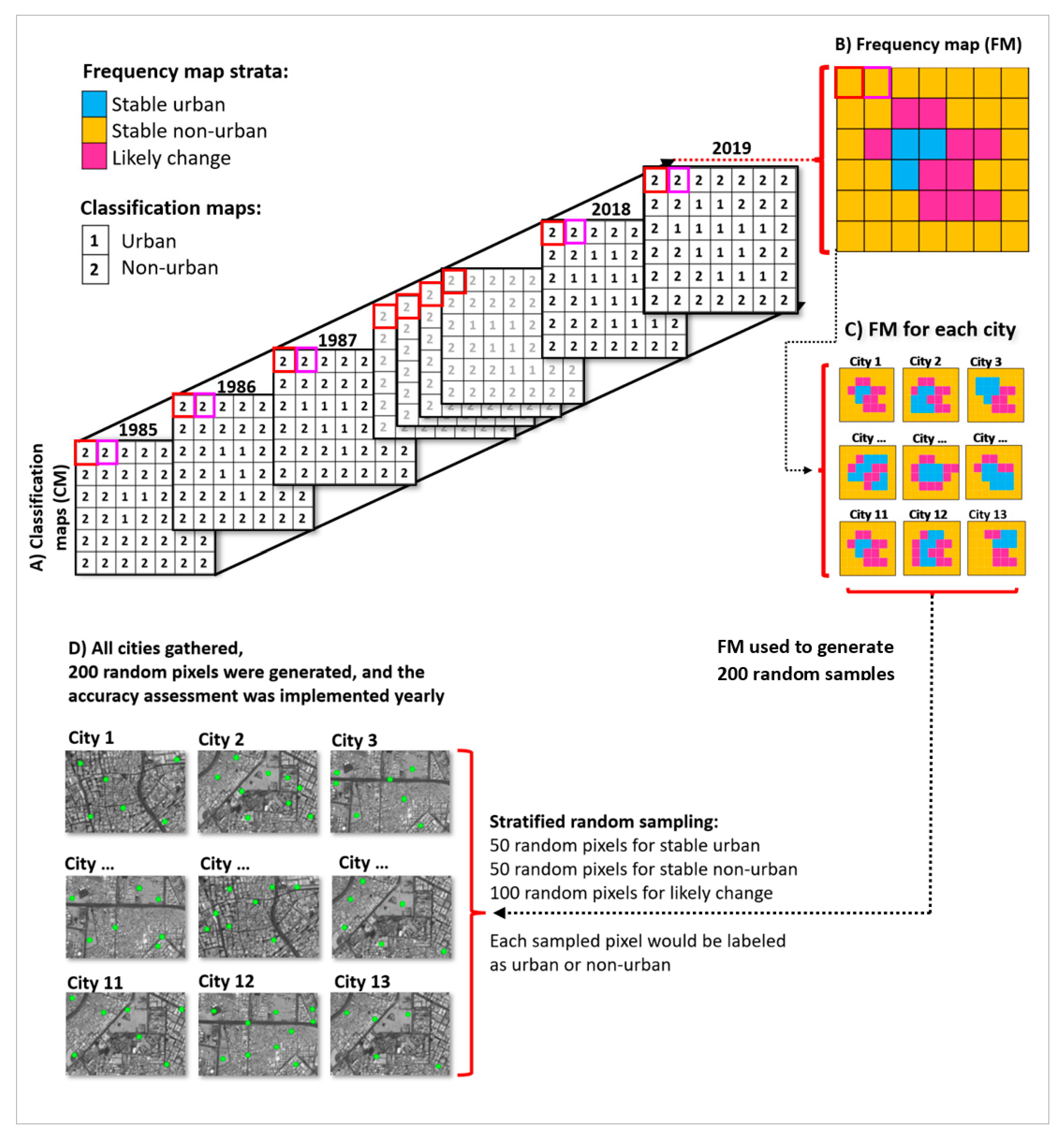
3.3. Estimating the Accuracy and Unbiased Area
3.4. Estimating Urban Expansion Rate and Intensity (1985–2019)
4. Results
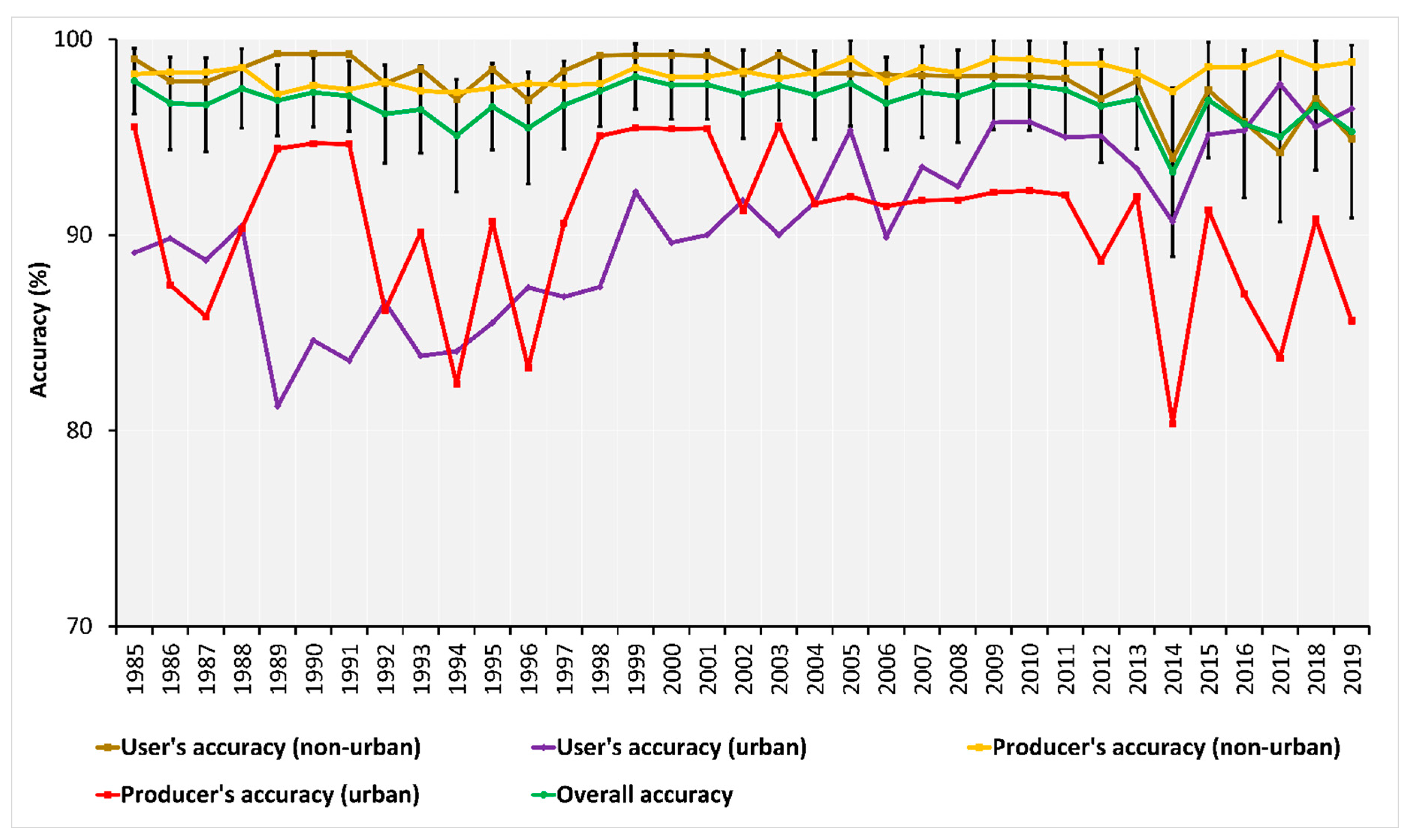
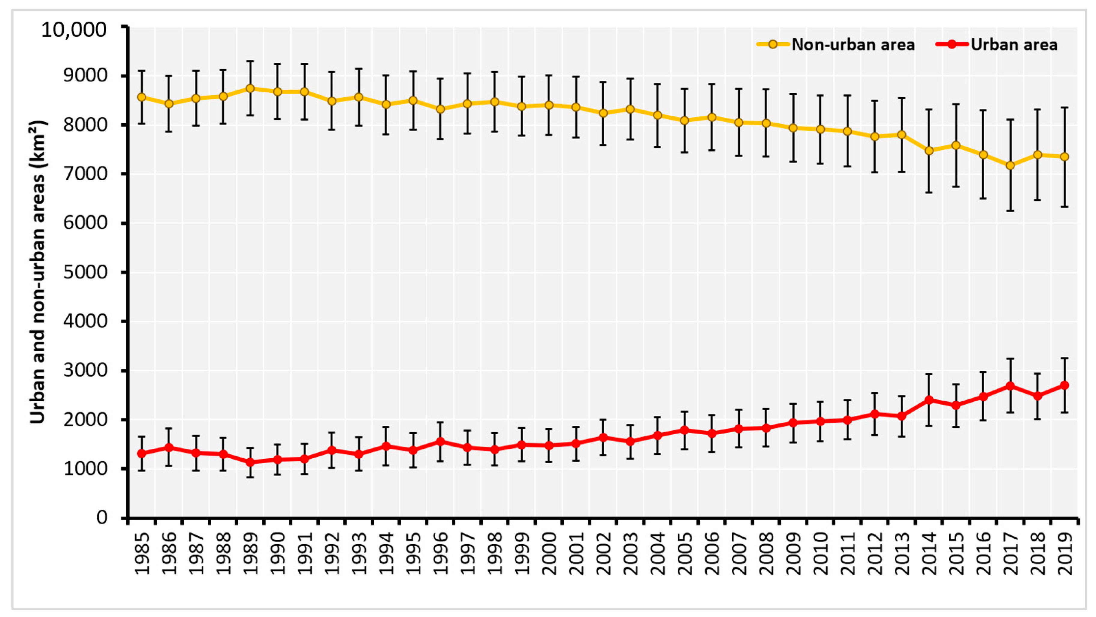
4.1. Accuracy Assessments and Unbiased Area Estimations
4.2. Characteristics of Urban Growth in Saudi Capital Cities (1985–2019)
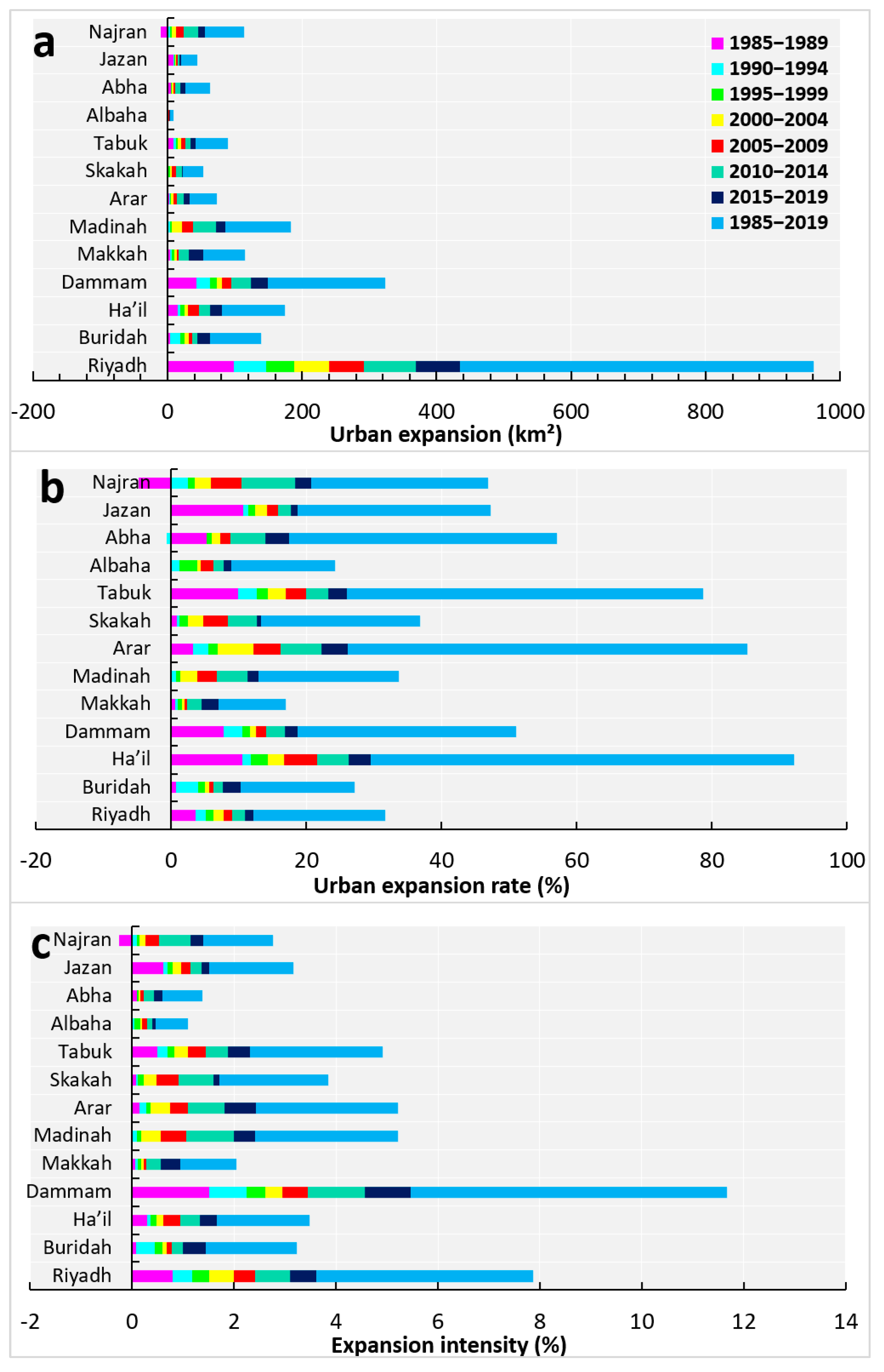
4.2.1. Urban Expansion Rate and Intensity
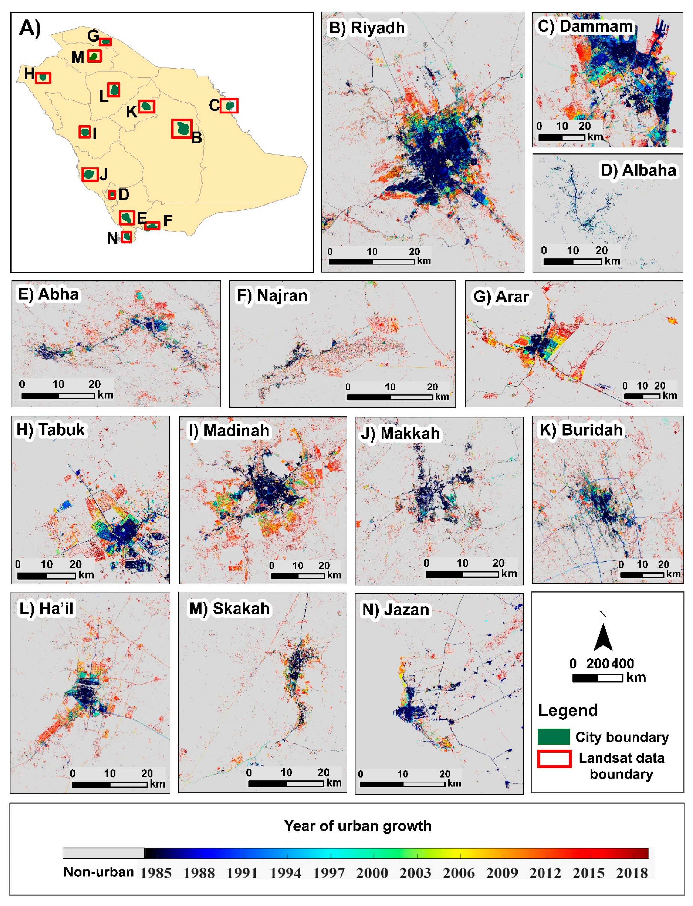
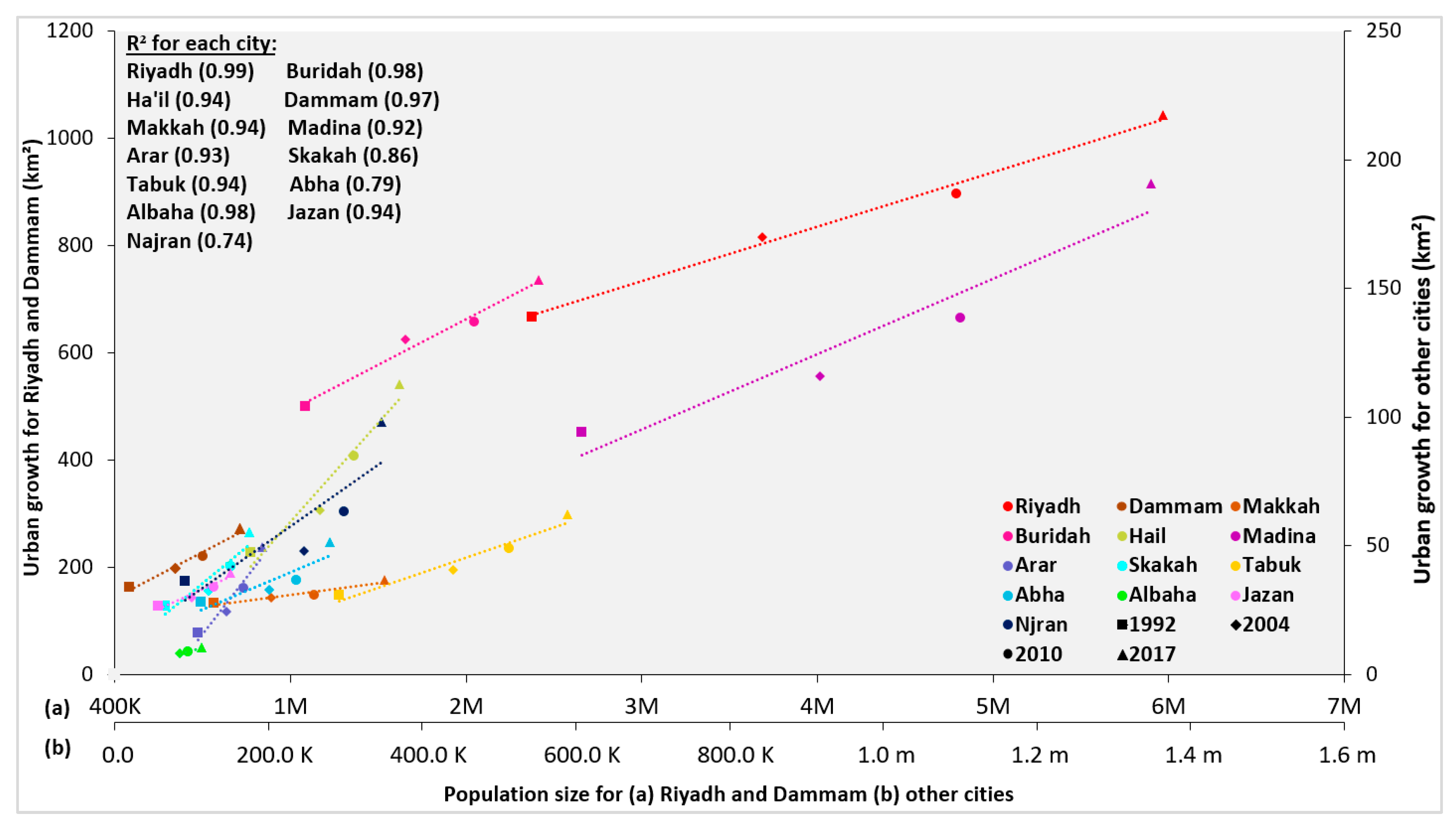
4.2.2. Spatial and Temporal Analysis for the 13 Capital Cities
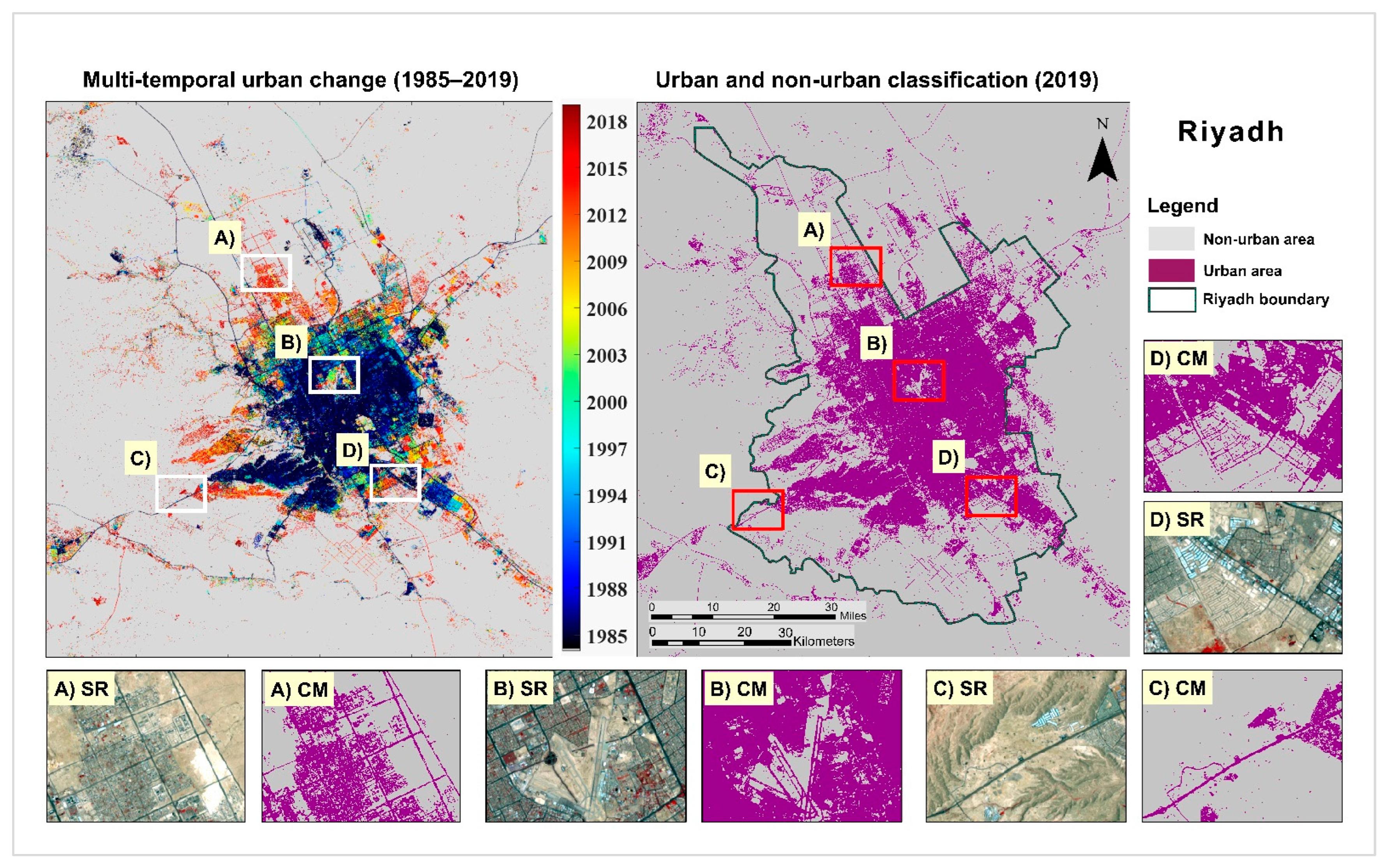
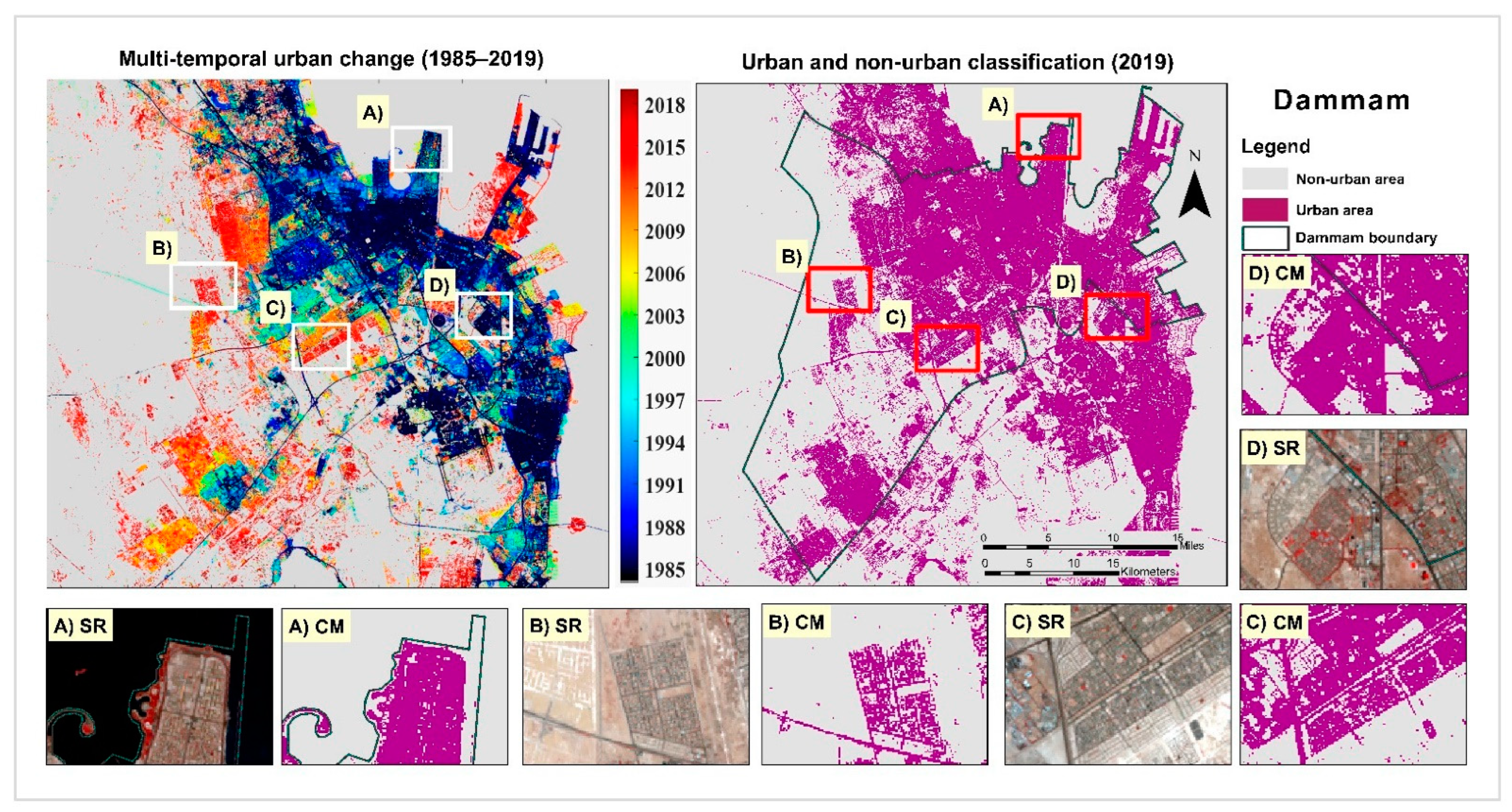
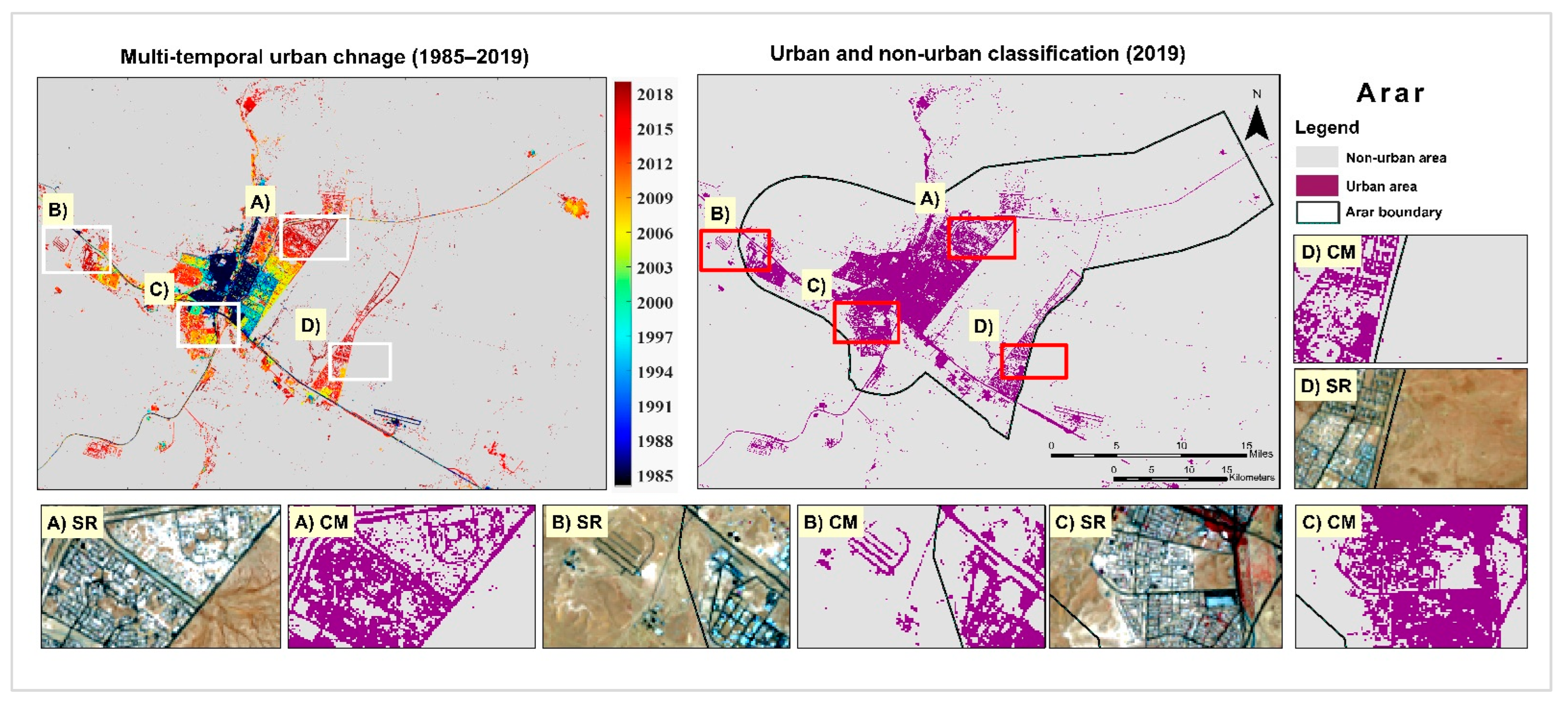
4.2.3. Examples of Riyadh, Dammam, and Arar
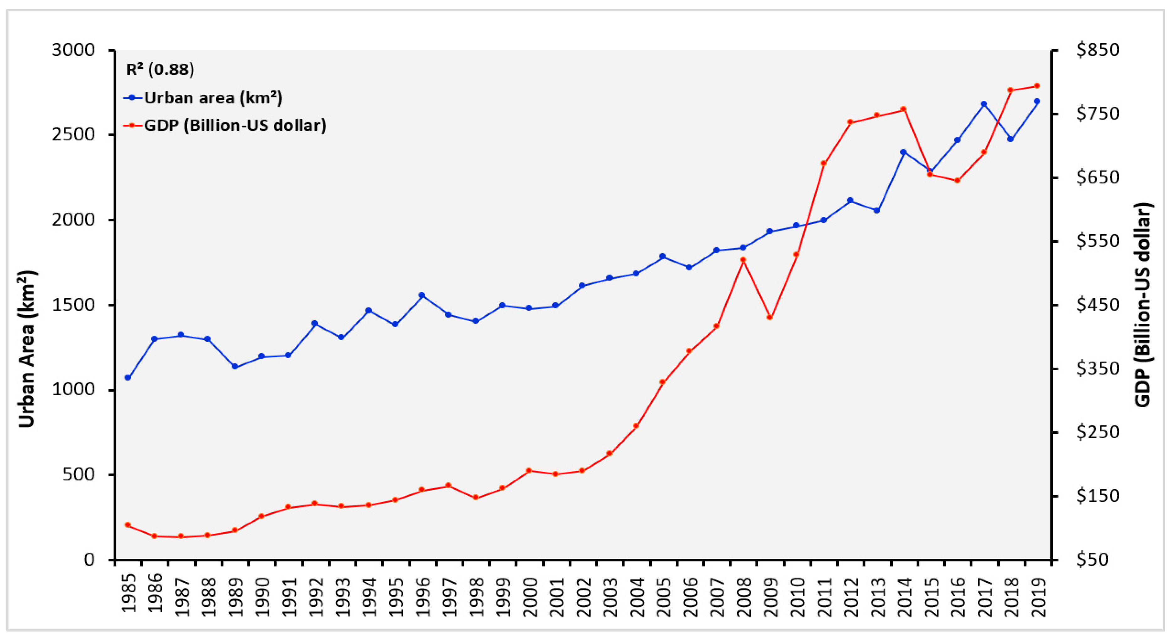
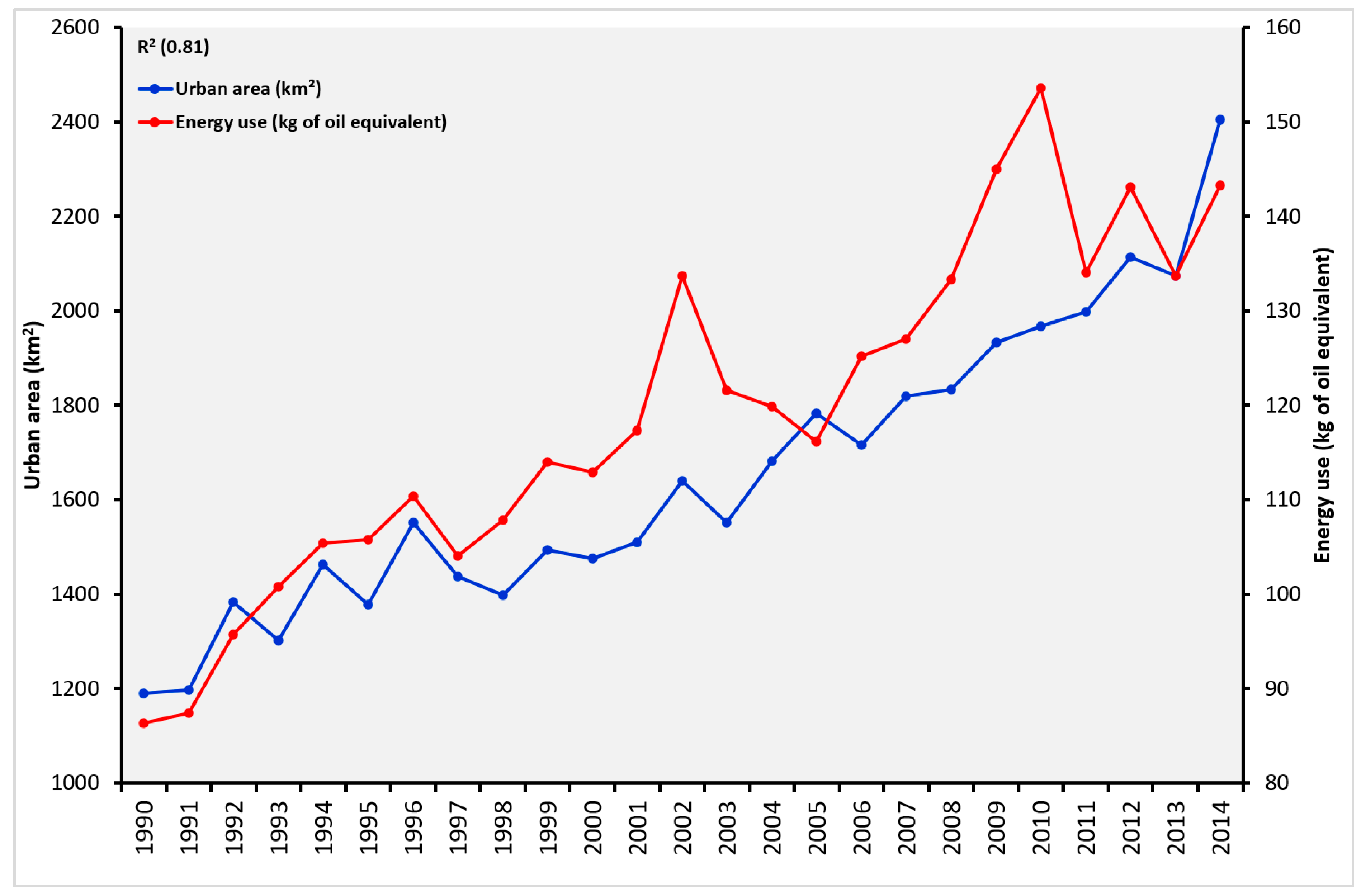
5. Discussion
6. Conclusions
Author Contributions
Funding
Institutional Review Board Statement
Informed Consent Statement
Data Availability Statement
Acknowledgments
Conflicts of Interest
References
- United Nations. World Population Prospects 2017—Data Booklet (ST/ESA/SER.A/401); United Nations: New York, NY, USA, 2017.
- Schneider, A.; Friedl, M.A.; Potere, D. Mapping global urban areas using MODIS 500-m data: New methods and datasets based on “urban ecoregions”. Remote Sens. Environ. 2010, 114, 1733–1746. [Google Scholar] [CrossRef]
- Sun, J.; Wang, H.; Song, Z.; Lu, J.; Meng, P.; Qin, S. Mapping essential urban land use categories in nanjing by integrating multi-source big data. Remote Sens. 2020, 12, 2386. [Google Scholar] [CrossRef]
- United Nations World’s Population Increasingly Urban with More Than Half Living in Urban Areas. Available online: https://www.un.org/en/development/desa/news/population/world-urbanization-prospects-2014.html (accessed on 2 January 2020).
- Kirabo Kacyira, A. Addressing the sustainable urbanization challenge. UN Chron. 2012, 49, 58–60. [Google Scholar] [CrossRef]
- Martine, G.; McGranahan, G.; Schensul, D.; Tacoli, C. Population Dynamics and Climate Change; UNFPA: New York, NY, USA, 2009; ISBN 9780897149198. [Google Scholar]
- Seto, K.C.; Güneralp, B.; Hutyra, L.R. Global forecasts of urban expansion to 2030 and direct impacts on biodiversity and carbon pools. Proc. Natl. Acad. Sci. USA 2012, 109, 16083–16088. [Google Scholar] [CrossRef] [PubMed] [Green Version]
- Seto, K.C.; Shobhakar, D.; Bigio, A.; Blanco, H.; Delgado, G.C.; Dewar, D.; Huang, L.; Inaba, A.; Kansal, A.; Lwasa, S.; et al. Human Settlements, Infrastructure, and Spatial Planning. In Climate Change 2014: Mitigation of Climate Change Working Group III Contribution to the IPCC Fifth Assessment Report; Cambridge University Press: Cambridge, UK, 2014; pp. 923–1000. [Google Scholar] [CrossRef] [Green Version]
- Defries, R.S.; Rudel, T.; Uriarte, M.; Hansen, M. Deforestation driven by urban population growth and agricultural trade in the twenty-first century. Nat. Geosci. 2010, 3, 178–181. [Google Scholar] [CrossRef]
- Hahs, A.K.; McDonnell, M.J.; McCarthy, M.A.; Vesk, P.A.; Corlett, R.T.; Norton, B.A.; Clemants, S.E.; Duncan, R.P.; Thompson, K.; Schwartz, M.W.; et al. A global synthesis of plant extinction rates in urban areas. Ecol. Lett. 2009, 12, 1165–1173. [Google Scholar] [CrossRef]
- Hobbie, S.E.; Finlay, J.C.; Benjamin, D.; Nidzgorski, D.A.; Millet, D.B.; Lawrence, A.; Hobbie, S.E.; Finlay, J.C.; Janke, B.D.; Nidzgorski, D.A.; et al. Correction: Contrasting nitrogen and phosphorus budgets in urban watersheds and implications for managing urban water pollution. Proc. Natl. Acad. Sci. USA 2017, 114, 4177–4182, Erratum in Proc. Natl. Acad. Sci. USA 2017, 114, E4116. [Google Scholar] [CrossRef] [Green Version]
- Liu, R.; Wang, M.; Chen, W.; Peng, C. Spatial pattern of heavy metals accumulation risk in urban soils of Beijing and its influencing factors. Environ. Pollut. 2016, 210, 174–181. [Google Scholar] [CrossRef]
- Ying, Q.; Hansen, M.C.; Potapov, P.V.; Tyukavina, A.; Wang, L.; Stehman, S.V.; Moore, R.; Hancher, M. Global bare ground gain from 2000 to 2012 using Landsat imagery. Remote Sens. Environ. 2017, 194, 161–176. [Google Scholar] [CrossRef] [Green Version]
- Zhang, H.; Wang, S.; Hao, J.; Wang, X.; Wang, S.; Chai, F.; Li, M. Air pollution and control action in Beijing. J. Clean. Prod. 2016, 112, 1519–1527. [Google Scholar] [CrossRef]
- Peng, S.; Piao, S.; Ciais, P.; Friedlingstein, P.; Ottle, C.; Bréon, F.M.; Nan, H.; Zhou, L.; Myneni, R.B. Response to comment on “Surface urban heat island across 419 global big cities”. Environ. Sci. Technol. 2012, 46, 6889–6890. [Google Scholar] [CrossRef]
- Buchhorn, M.; Bertels, L.; Smets, B.; De Roo, B.; Lesiv, M.; Tsendbazar, N.; Masiliunas, D.; Linlin, L. Copernicus Global Land Operations “Vegetation and Energy”; “CGLOPS-1” Framework Service Contract N° 199494 (JRC) Algorithm Theoretical Basis Document Moderate Dynamic Land Cover Collection 100 M Version 3 Issue 3.4; Zenodo: Geneva, Switzerland, 2021. [Google Scholar] [CrossRef]
- Huang, X.; Huang, J.; Wen, D.; Li, J. An updated MODIS global urban extent product (MGUP) from 2001 to 2018 based on an automated mapping approach. Int. J. Appl. Earth Obs. Geoinf. 2021, 95, 102255. [Google Scholar] [CrossRef]
- Friedl, M.A.; Sulla-Menashe, D.; Tan, B.; Schneider, A.; Ramankutty, N.; Sibley, A.; Huang, X. MODIS Collection 5 global land cover: Algorithm refinements and characterization of new datasets. Remote Sens. Environ. 2010, 114, 168–182. [Google Scholar] [CrossRef]
- Sulla-Menashe, D.; Gray, J.M.; Abercrombie, S.P.; Friedl, M.A. Hierarchical mapping of annual global land cover 2001 to present: The MODIS Collection 6 Land Cover product. Remote Sens. Environ. 2019, 222, 183–194. [Google Scholar] [CrossRef]
- Zhou, Y.; Smith, S.J.; Zhao, K.; Imhoff, M.; Thomson, A.; Bond-Lamberty, B.; Asrar, G.R.; Zhang, X.; He, C.; Elvidge, C.D. A global map of urban extent from nightlights. Environ. Res. Lett. 2015, 10, 054011. [Google Scholar] [CrossRef]
- Bartholomé, E.; Belward, A.S. GLC2000: A new approach to global land cover mapping from earth observation data. Int. J. Remote Sens. 2005, 26, 1959–1977. [Google Scholar] [CrossRef]
- Bicheron, P.; Defourny, P.; Brockmann, C.; Schouten, L.; Vancutsem, C.; Huc, M.; Bontemps, S.; Leroy, M.; Achard, F.; Herold, M.; et al. GLOBCOVER Products Description Manual ESA GlobCover Project Led by Medias France. Available online: https://publications.jrc.ec.europa.eu/repository/handle/JRC49240 (accessed on 15 January 2020).
- CIESIN Global Rural-Urban Mapping Project, Version 1 (GRUMPv1): Urban Extents Grid; NASA Socioeconomic Data and Applications Center (SEDAC): Palisades, NY, USA; Available online: https://sedac.ciesin.columbia.edu/data/set/grump-v1-urban-extents (accessed on 15 January 2020).
- Elvidge, C.D.; Tuttle, B.T.; Sutton, P.S.; Baugh, K.E.; Howard, A.T.; Milesi, C.; Bhaduri, B.L.; Nemani, R. Global distribution and density of constructed impervious surfaces. Sensors 2007, 7, 1962–1979. [Google Scholar] [CrossRef]
- Schneider, A.; Friedl, M.A.; Potere, D. A new map of global urban extent from MODIS satellite data. Environ. Res. Lett. 2009, 4, 2000–2010. [Google Scholar] [CrossRef] [Green Version]
- Florczyk, A.J.; Melchiorri, M.; Orbane, C.; Schiavina, M.; Maffenini, M.; Politis, P.; Sabo, S.; Freire, S.; Ehrlich, D.; Kemper, T.; et al. Description of the GHS Urban Centre Database 2015; Publications Office of the European Union: Luxembourg, 2019; p. 79. [CrossRef]
- Small, C. A global analysis of urban reflectance. Int. J. Remote Sens. 2005, 26, 661–681. [Google Scholar] [CrossRef]
- Gong, P.; Li, X.; Wang, J.; Bai, Y.; Chen, B.; Hu, T.; Liu, X.; Xu, B.; Yang, J.; Zhang, W.; et al. Annual maps of global artificial impervious area (GAIA) between 1985 and 2018. Remote Sens. Environ. 2020, 236, 111510. [Google Scholar] [CrossRef]
- Gong, P.; Li, X.; Zhang, W. 40-Year (1978–2017) human settlement changes in China reflected by impervious surfaces from satellite remote sensing. Sci. Bull. 2019, 64, 756–763. [Google Scholar] [CrossRef] [Green Version]
- Population and Housing Census. Available online: https://www.stats.gov.sa/en/13 (accessed on 15 January 2020).
- Saudi Oil Production Policy. Available online: https://www.moenergy.gov.sa/arabic/ministry/Pages/petroleum-and-politics.aspx (accessed on 3 March 2020).
- The Energy. Available online: https://www.moenergy.gov.sa/arabic/Energy/Pages/petroleum.aspx (accessed on 7 January 2020).
- Abdelatti, H.; Elhadary, Y.; Babiker, A.A. Nature and Trend of Urban Growth in Saudi Arabia: The Case of Al-Ahsa Province—Eastern Region. Resour. Environ. 2017, 7, 69–80. [Google Scholar] [CrossRef]
- Alhowaish, A.K. Eighty years of urban growth and socioeconomic trends in Dammam Metropolitan Area, Saudi Arabia. Habitat Int. 2015, 50, 90–98. [Google Scholar] [CrossRef]
- Al-Shihri, F.S. Impacts of large-scale residential projects on urban sustainability in Dammam Metropolitan Area, Saudi Arabia. Habitat Int. 2016, 56, 201–211. [Google Scholar] [CrossRef]
- Aljoufie, M.; Zuidgeest, M.; Brussel, M.; van Maarseveen, M. Spatial-temporal analysis of urban growth and transportation in Jeddah City, Saudi Arabia. Cities 2013, 31, 57–68. [Google Scholar] [CrossRef]
- Jamali, N.A.; Rahman, M.T. Utilization of Remote Sensing and GIS to Examine Urban Growth in the City of Riyadh, Saudi Arabia. J. Adv. Inf. Technol. 2016, 7, 297–301. [Google Scholar] [CrossRef]
- Aljaddani, A. Integration of Multi-Temporal Remote Sensing Imagery and GIS Mapping and Analysis of Land Use Change in Jeddah City, Saudi Arabia. Ph.D. Thesis, Murray State University, Murray, KY, USA, 2015. [Google Scholar]
- Abdulrazzak, M.J. Water Supplies versus Demand in Countries of Arabian Peninsula. J. Water Resour. Plan. Manag. 1995, 121, 227–234. [Google Scholar] [CrossRef]
- Saudi Census. Available online: https://www.stats.gov.sa/sites/default/files/population_by_age_groups_and_gender_ar.pdf (accessed on 15 January 2020).
- Abdul Salam, A.; Elsegaey, I.; Khraif, R.; Al-Mutairi, A. Population distribution and household conditions in Saudi Arabia: Reflections from the 2010 Census. Springerplus 2014, 3, 1–13. [Google Scholar] [CrossRef] [Green Version]
- National Geological Database (NGD). Available online: https://ngd.sgs.org.sa/en (accessed on 10 August 2019).
- Saeed, T.M.; Al-Dashti, H.; Spyrou, C. Aerosol’s optical and physical characteristics and direct radiative forcing during a shamal dust storm, a case study. Atmos. Chem. Phys. 2014, 14, 3751–3769. [Google Scholar] [CrossRef] [Green Version]
- Al Tokhais, A.S.; Rausch, R. The Hydrogeology of Al Hassa Springs. In Proceedings of the Third International Conference on Water Resources and Arid Environments (2008) and the First Arab Water Forum, Riyadh, Saudi Arabia, 16–19 November 2008. [Google Scholar]
- Abha. Available online: https://unhabitat.org/sites/default/files/2020/05/abha.pdf (accessed on 15 January 2020).
- Krishna, V. Long Term Temperature Trends in Four Different Climatic Zones of Saudi Arabia. Int. J. Appl. Sci. Technol. 2014, 4, 233–242. [Google Scholar]
- U.S. Geological Survey. Available online: https://espa.cr.usgs.gov/ (accessed on 19 August 2019).
- Masek, J.G.; Vermote, E.F.; Saleous, N.E.; Wolfe, R.; Hall, F.G.; Huemmrich, K.F.; Gao, F.; Kutler, J.; Lim, T.K. A landsat surface reflectance dataset for North America, 1990–2000. IEEE Geosci. Remote Sens. Lett. 2006, 3, 68–72. [Google Scholar] [CrossRef]
- Vermote, E.F.; El Saleous, N.; Justice, C.O.; Kaufman, Y.J.; Privette, J.L.; Remer, L.; Roger, J.C.; Tanré, D. Atmospheric correction of visible to middle-infrared EOS-MODIS data over land surfaces: Background, operational algorithm and validation. J. Geophys. Res. Atmos. 1997, 102, 17131–17141. [Google Scholar] [CrossRef] [Green Version]
- Townshend, J.R.; Masek, J.G.; Huang, C.; Vermote, E.F.; Gao, F.; Channan, S.; Sexton, J.O.; Feng, M.; Narasimhan, R.; Kim, D.; et al. Global characterization and monitoring of forest cover using Landsat data: Opportunities and challenges. Int. J. Digit. Earth 2012, 5, 373–397. [Google Scholar] [CrossRef] [Green Version]
- Vermote, E.; Justice, C.; Claverie, M.; Franch, B. Preliminary analysis of the performance of the Landsat 8/OLI land surface reflectance product. Remote Sens. Environ. 2016, 185, 46–56. [Google Scholar] [CrossRef]
- Zhu, Z.; Wang, S.; Woodcock, C.E. Improvement and expansion of the Fmask algorithm: Cloud, cloud shadow, and snow detection for Landsats 4–7, 8, and Sentinel 2 images. Remote Sens. Environ. 2015, 159, 269–277. [Google Scholar] [CrossRef]
- Zhu, Z.; Woodcock, C.E. Object-based cloud and cloud shadow detection in Landsat imagery. Remote Sens. Environ. 2012, 118, 83–94. [Google Scholar] [CrossRef]
- Zhu, Z.; Woodcock, C.E.; Holden, C.; Yang, Z. Generating synthetic Landsat images based on all available Landsat data: Predicting Landsat surface reflectance at any given time. Remote Sens. Environ. 2015, 162, 67–83. [Google Scholar] [CrossRef]
- Zhu, Z.; Woodcock, C.E. Continuous change detection and classification of land cover using all available Landsat data. Remote Sens. Environ. 2014, 144, 152–171. [Google Scholar] [CrossRef] [Green Version]
- Anderson, J.; Hardy, E.; Roach, J.; Witmer, R. A Land Use and Land Cover Classification System for Use with Remote Sensor Data; US Government Printing Office: Washington, DC, USA, 1976; Volume 964.
- Breiman, L. Random forests. In Hands-On Machine Learning with R; Chapman and Hall/CRC: London, UK, 2001; pp. 1–122. [Google Scholar] [CrossRef]
- Olofsson, P.; Foody, G.M.; Herold, M.; Stehman, S.V.; Woodcock, C.E.; Wulder, M.A. Good practices for estimating area and assessing accuracy of land change. Remote Sens. Environ. 2014, 148, 42–57. [Google Scholar] [CrossRef]
- Buja, K. Sampling Design Tool (ArcGIS 10.4.1). Available online: https://www.arcgis.com/home/item.html?id=28f08ca526ae44e8ac107a2a0d5f50e3 (accessed on 20 April 2020).
- Olofsson, P.; Foody, G.M.; Stehman, S.V.; Woodcock, C.E. Making better use of accuracy data in land change studies: Estimating accuracy and area and quantifying uncertainty using stratified estimation. Remote Sens. Environ. 2013, 129, 122–131. [Google Scholar] [CrossRef]
- Jenness, J.; Wynne, J. Cohen’s Kappa and Classification Table Metrics 2.0: An ArcView 3x Extension for Accuracy Assessment of Spatially Explicit Models; Southwest Biological Science Center Open-File Report; U.S. Geological Survey, Southwest Biological Science Center: Flagstaff, AZ, USA, 2005. [CrossRef]
- Xu, X.; Min, X. Quantifying spatiotemporal patterns of urban expansion in China using remote sensing data. Cities 2013, 35, 104–113. [Google Scholar] [CrossRef]
- Chen, K.; Zhang, F.; Du, Z.; Liu, R. Analysis of urban expansion and driving forces in Jiaxing city based on remote sensing image. J. China Univ. Min. Technol. China Univ. Min. Technol. 2007, 17, 267–271. [Google Scholar] [CrossRef]
- Sun, C.; Wu, Z.F.; Lv, Z.Q.; Yao, N.; Wei, J.B. Quantifying different types of urban growth and the change dynamic in Guangzhou using multi-temporal remote sensing data. Int. J. Appl. Earth Obs. Geoinf. 2013, 21, 409–417. [Google Scholar] [CrossRef]
- Alqurashi, A.F.; Kumar, L.; Sinha, P. Urban land cover change modelling using time-series satellite images: A case study of urban growth in five cities of Saudi Arabia. Remote Sens. 2016, 8, 838. [Google Scholar] [CrossRef] [Green Version]
- Saudi Arabia-Major Cities. Available online: https://www.citypopulation.de/en/saudiarabia/cities/ (accessed on 9 September 2020).
- The World Bank. Available online: https://data.worldbank.org/indicator/NY.GDP.MKTP.CD?locations=SA (accessed on 9 January 2020).
- The Performance of the Housing Sector during the Corona Pandemic. 2020. Available online: https://hdoc.sa/en-us/Pages/NewsLetters.aspx (accessed on 20 February 2020).
- The World Bank. Available online: https://data.worldbank.org/indicator/EG.USE.COMM.GD.PP.KD?locations=SA (accessed on 1 May 2022).
- Zhang, C.; Chen, Y.; Lu, D. Mapping the land-cover distribution in arid and semiarid urban landscapes with Landsat Thematic Mapper imagery. Int. J. Remote Sens. 2015, 36, 4483–4500. [Google Scholar] [CrossRef]
- Rasul, A.; Balzter, H.; Ibrahim, G.R.F.; Hameed, H.M.; Wheeler, J.; Adamu, B.; Ibrahim, S.; Najmaddin, P.M. Applying built-up and bare-soil indices from Landsat 8 to cities in dry climates. Land 2018, 7, 81. [Google Scholar] [CrossRef] [Green Version]
- Chen, J.; Chen, J.; Liao, A.; Cao, X.; Chen, L.; Chen, X.; He, C.; Han, G.; Peng, S.; Lu, M.; et al. Global land cover mapping at 30 m resolution: A POK-based operational approach. ISPRS J. Photogramm. Remote Sens. 2015, 103, 7–27. [Google Scholar] [CrossRef] [Green Version]
- Landsat Known Issues. Available online: https://www.usgs.gov/land-resources/nli/landsat/landsat-known-issues (accessed on 10 July 2020).
- Aljaddani, A.; Song, X.-P.; Zhu, Z. Saudi Arabian Capitals Urban Land Cover Maps: 1985–2019. Version: 1. Available online: https://zenodo.org/record/6210073#.Yn_bJ-jMKF4 (accessed on 21 February 2022).
- Zhu, Z. GERSL–CCDC. Available online: https://github.com/GERSL/CCDC (accessed on 8 August 2019).


| City Name | Urban Pixels | Non-Urban Pixels | City Size (km × km) | Date | Path/Row |
|---|---|---|---|---|---|
| Riyadh | 232,609 | 534,025 | 83.49 × 97.74 | 2013 | 165/043 |
| Buridah | 76,259 | 1,327,780 | 47.34 × 50.37 | 2014 | 168/042 |
| Ha’il | 42,245 | 1,293,491 | 49.74 × 64.14 | 2005 | 169/041 |
| Dammam | 231,310 | 71,966 | 40.59 × 40.47 | 2014 | 163/042 |
| Makkah | 39,121 | 518,555 | 61.11 × 54.21 | 2013 | 169/045 |
| Madinah | 51,394 | 374,444 | 38.43 × 40.68 | 2005 | 170/043 |
| Arar | 11,461 | 352,432 | 37.05 × 25.5 | 2004 | 170/039 |
| Skakah | 15,566 | 730,318 | 43.08 × 42.84 | 2003 | 171/039 |
| Tabuk | 29,155 | 511,715 | 28.2 × 31.5 | 2005 | 173/040 |
| Albaha | 3054 | 91,936 | 25.32 × 23.52 | 2002 | 168/046 |
| Abha | 11,464 | 318,887 | 77.43 × 68.91 | 2013 | 167/047 |
| Jazan | 13,093 | 160,557 | 32.52 × 39.69 | 2010 | 167/048 |
| Najran | 45,726 | 953,402 | 86.25 × 45.33 | 2015 | 166/048 |
| Total pixels | 802,457 | 7,239,508 |
| Reference Data | |||||
|---|---|---|---|---|---|
| Stable Non-Urban | Stable Urban | Change | Total | ||
| Classified map | Stable non-urban | 0.685 | 0.000 | 0.044 | 0.728 |
| Stable urban | 0.002 | 0.083 | 0.024 | 0.109 | |
| Change | 0.018 | 0.003 | 0.141 | 0.162 | |
| Total | 0.705 | 0.086 | 0.209 | 1.000 | |
| Area (km2) | 2064.075 | ||||
| ±95% CI (km2) | 571.663 | ||||
| User’s accuracy | 0.94 | 0.76 | 0.87 | ||
| Producer’s accuracy | 0.97 | 0.96 | 0.68 | ||
| Overall accuracy | 0.91 | ||||
Publisher’s Note: MDPI stays neutral with regard to jurisdictional claims in published maps and institutional affiliations. |
© 2022 by the authors. Licensee MDPI, Basel, Switzerland. This article is an open access article distributed under the terms and conditions of the Creative Commons Attribution (CC BY) license (https://creativecommons.org/licenses/by/4.0/).
Share and Cite
Aljaddani, A.H.; Song, X.-P.; Zhu, Z. Characterizing the Patterns and Trends of Urban Growth in Saudi Arabia’s 13 Capital Cities Using a Landsat Time Series. Remote Sens. 2022, 14, 2382. https://doi.org/10.3390/rs14102382
Aljaddani AH, Song X-P, Zhu Z. Characterizing the Patterns and Trends of Urban Growth in Saudi Arabia’s 13 Capital Cities Using a Landsat Time Series. Remote Sensing. 2022; 14(10):2382. https://doi.org/10.3390/rs14102382
Chicago/Turabian StyleAljaddani, Amal H., Xiao-Peng Song, and Zhe Zhu. 2022. "Characterizing the Patterns and Trends of Urban Growth in Saudi Arabia’s 13 Capital Cities Using a Landsat Time Series" Remote Sensing 14, no. 10: 2382. https://doi.org/10.3390/rs14102382