
Efficient Shallow Network for River Ice Segmentation


Department of Systems Design Engineering, University of Waterloo, Waterloo, ON N2L G31, Canada
*
Author to whom correspondence should be addressed.
Remote Sens. 2022, 14(10), 2378; https://doi.org/10.3390/rs14102378
Submission received: 16 March 2022
/
Revised: 22 April 2022
/
Accepted: 10 May 2022
/
Published: 15 May 2022
(This article belongs to the Topic Big Data and Artificial Intelligence)
Abstract
:River ice segmentation, used for surface ice concentration estimation, is important for validating river processes and ice-formation models, predicting ice jam and flooding risks, and managing water supply and hydroelectric power generation. Furthermore, discriminating between anchor ice and frazil ice is an important factor in understanding sediment transport and release events. Modern deep learning techniques have proved to deliver promising results; however, they can show poor generalization ability and can be inefficient when hardware and computing power is limited. As river ice images are often collected in remote locations by unmanned aerial vehicles with limited computation power, we explore the performance-latency trade-offs for river ice segmentation. We propose a novel convolution block inspired by both depthwise separable convolutions and local binary convolutions giving additional efficiency and parameter savings. Our novel convolution block is used in a shallow architecture which has 99.9% fewer trainable parameters, 99% fewer multiply–add operations, and 69.8% less memory usage than a UNet, while achieving virtually the same segmentation performance. We find that the this network trains fast and is able to achieve high segmentation performance early in training due to an emphasis on both pixel intensity and texture. When compared to very efficient segmentation networks such as LR-ASPP with a MobileNetV3 backbone, we achieve good performance (mIoU of 64) 91% faster during training on a CPU and an overall mIoU that is 7.7% higher. We also find that our network is able to generalize better to new domains such as snowy environments.
1. Introduction
Due to recent advancements, deep learning has become a powerful tool in the segmentation of remote sensing imagery. Image segmentation extended to river ice is an important step in estimating surface ice concentration for validating river process and ice-formation models [1]. Information regarding river ice can also be integral for water supply management, hydroelectric power generation [2], and predicting ice jam risks [3]. Furthermore, discriminating between different classes of ice, such as surface-forming frazil ice and sediment-rich anchor ice, can be important in understanding sediment transport and release events [4].
The first ice type of interest, frazil ice, forms as ice crystals flocculate together, float to the surface forming surface slush, and consolidate to form frazil ice pans. In the late stages of freeze up, frazil ice pans can freeze together to form frazil ice rafts. Frazil ice pans often appear circular and can have upturned edges caused by collisions with other ice pans. The second ice type of interest, anchor ice, forms on river beds, resulting in a high sediment content within the ice. Through thermal or mechanical means, the anchor ice can be released from the river bed and float to the surface [4]. On the surface, anchor ice usually appears darker than frazil ice due to the high sediment content, and may have fewer upturned edges due to less time on the surface and different structural properties. When anchor ice release events occur, frazil ice generation may have already stopped. This can result in a much higher concentration of anchor ice than frazil ice [4].
The Peace River flows from the Rocky Mountains of British Columbia in Western Canada to the Northeast corner of Alberta, Canada, where it forms the Peace–Athabasca Delta, the largest boreal freshwater ecosystem in the world and a UNESCO World Heritage Site [5]. A study regarding suspended load mass flux in the Peace River determined that with a mean annual flow of 1600 m/s, there was a constant suspended sediment load of 1204 kg/s [6]. Another study found that a sediment mass flux of up to 421 kg/s can be attributed to ice rafting during anchor ice release events, accounting for up to 3.3% of the total annual suspended sediment transported assuming 30 anchor ice release events in a year [7]. The same study also noted that during an anchor ice release event, the anchor ice rafting may account for up to 40% of average suspended max. flux. With estimates of the sediment concentration within anchor ice pans [8], meaningful contributions can be made to the annual sediment budget by efficiently imaging and segmenting anchor ice pans during anchor ice release events.
One means of collecting imagery of anchor ice is through the use of an unmanned aerial vehicles (UAVs) [1,4,9,10,11]. Due to the limited hardware aboard many UAVs, data-intensive processes, such as deep learning algorithms, which require large computing and memory resources, are difficult to implement in real time. When operating on UAV data in real time, the information collected on the UAV can be sent to a remote processing device; however, this requires a wireless link with high bandwidth, minimal latency, and ultra-reliable connection [12]; therefore, it may not be possible in remote regions. Alternatively, data can be processed on the UAV itself, although depending on the model of the UAV this would involve a low/middle grade GPU [13] or no GPU at all. This computation obstacle is also present in other domains such as forest fire detection [14], crop phenology [15], and sea ice segmentation [16] where computation limitations hinder operational sea ice prediction [17].
Promising results have been achieved by applying deep learning to the task of river ice segmentation, particularly for discriminating between frazil and anchor ice, where convolutional neural networks (CNNs) greatly outperformed previously used support vector machines (SVMs) [1,4]. One downfall of these deep learning methods lies in their ability to generalize to data that differs from the training domain [1]. Additionally, little focus has been put on the efficiency of these networks in both training and inference. Although deep learning has shown promise for the task of river ice segmentation, it bears the question of if these favourable results can be attained when inference data differs significantly from training data and when training and inference happen in real time. As there is an inherent trade-off between performance and latency in the field of deep learning, we aim to build a network architecture that preserves performance while doing so efficiently, enabling more convenient river ice segmentation on edge devices such as a UAV.
2. Background
2.1. River Ice Segmentation
Various techniques have been used for river ice segmentation, including traditional image processing [18], machine learning models [4,9,19,20], and deep learning solutions [1,10,11]. Recent studies hlhave chosen to utilize deep learning models over other image processing and machine learning techniques as deep learning solutions have been proven to perform better, especially when tasks become more complicated [4]. Specifically, for a dataset with both frazil and anchor ice, an SVM performed well in differentiating ice from water, but when attempting the more difficult task of segmenting frazil ice, anchor ice, and water, the SVM achieved low segmentation accuracy [4]. On the same task of segmenting frazil ice, anchor ice, and water, a suite of deep learning models outperformed the SVM [1]. The authors found that two neural network architectures, DeepLabV3+ [21] and UNet [22], outperformed the SVM for all three classes. They found that although DeepLabV3+ outperformed UNet with regards to quantitative metrics on a labelled test set, DeepLabV3+ showed poor generalization ability upon visual inspection of model results on unlabelled data. The authors concluded that UNet provided the best trade-off between quantitative scores on a labelled test set and qualitative results on unlabelled data.
2.2. Depthwise Separable Convolution
Depthwise separable convolutions (DSCs) are key components of modern efficient networks. Many efficient networks replace standard convolution operations in common network architectures with DSCs, resulting in a significant increase in efficiency while minimizing performance losses [23,24,25,26,27].
If we let h and w be the height and width of a feature map, and be the number of input and output channels of a convolution, and k be the kernel size, a standard convolution takes an input of size and gives an output of size assuming the input and output feature maps have the same spatial dimensions. The kernel of a standard convolution is of size , meaning there are filters of size [23].
DSCs split standard convolution operations into two parts, a depthwise convolution and a pointwise convolution. The depthwise convolution occurs first and is similar to a standard convolution; however, it only applies a single unique filter to each channel of the input image or feature map. Using the same variables as defined previously, this means that the depthwise convolution has filters of size . The depthwise convolution is followed by the pointwise convolution, which is a 1 × 1 convolution across depth, allowing for a change in the number of channels of the output feature map if desired.
Again using the same variables as defined previously, the computational cost of a standard convolution operation is therefore
while the computational cost of a DSC is
as calculated by adding the cost of the depthwise and pointwise parts of the convolution [26].
As a result, DSCs reduce computational cost by a factor of or approximately when . Therefore, when using a kernel size of , computational cost is reduced by 8 to 9 times by using DSCs. The trade-off in performance was found to be minimal in a study where a network was built with DSCs had an ImageNet accuracy of 70.6% and 569M Mult-Adds, while an identical network with standard convolutions had an ImageNet accuracy of 71.7% and 4866M Mult-Adds [23].
2.3. Local Binary Convolution
Local binary convolutions (LBCs) are another alternative to a standard convolution that significantly reduces the number of trainable parameters [28]. LBCs are inspired by local binary patterns (LBPs), which are texture pattern descriptors used to characterize local texture patterns in an image based on a neighbourhood of pixels [29]. Based on contrasting pixels in a neighbourhood, a string of bits is calculated and converted to a base 2 decimal number which is used as the feature to the central pixel. An LBP for a window can be calculated as follows,
where is the intensity of the centre pixel at location , and is the the intensity of the nth neighbouring pixel out of N total neighbours. LBPs are illumination invariant as they focus on contrasting pixels which describe texture. As a result, they have become a popular image descriptor for facial recognition tasks, among others [30].
Similar to DSCs, LBCs also operate in two stages; first a spatial convolution, and second a channel-wise convolution. The first stage, , modifies a standard convolution such that the kernel weights , which are still of size (recall that this is in contrast to the depthwise stage of a DSC, where weights are of size , or a single unique filter is applied to each channel of the input. The first stage in a LBC applies multiple filters to each channel of the input similar to a standard convolution), are non-trainable and randomly initialized such that . More specifically, to determine the arrangement of −1, 0, and 1 in , a sparsity proportion, , is set which determines the amount of non-zero values in . This involves setting of to zero according to a random uniform distribution (note that we follow the same convention as the LBCNN authors where the sparsity percentage refers to the percentage of non-zero elements i.e., sparsity = 100% corresponds to a dense weight tensor [28]). Then, the remaining non-zero values are randomly assigned to or 1 with equal probability using a Bernoulli distribution. The output of is then passed through an activation function (sigmoid or ReLU), and used as an input to the second stage, . Again similar to DSCs, consists of a convolution that acts only on the channels of the feature maps and contains the only trainable parameters in LBCs.
Using the same variable definitions in Section 2.2, a standard convolution operation has trainable parameters, while a LBC operation only has trainable parameters since in the convolution (note that this calculation assumes that outputs the same number of channels as are in the input to ).
2.4. Efficient Networks
Since the introduction of DSCs for efficient networks, various architectures have been developed, including the suite of MobileNets (V1, V2, V3) [23,26,27], MnasNet [31], and others. The latest of the aforementioned networks, MobileNetV3, borrows various aspects from other networks as well as introduces advancements of its own. MobileNetV3 uses DSCs from MobileNetV1, a linear bottleneck and inverted residual structure from MobileNetV2, and lightweight attention modules based on squeeze and excitation from MnasNet. Novel contributions of MobileNetV3 include a hardware-aware network architecture search, the h-swish nonlinearity, and rearrangement of computationally expensive layers at the beginning and end of the network [27].
For the task of semantic segmentation, MobileNetV3 can be used as a backbone feature extractor in a segmentation network such as DeepLabV3 [32]. The authors of MobileNetV2 designed a reduced Atrous Spatial Pyramid Pooling module [33] that was found to outperform the standard DeepLabV3. MobileNetV3 designed a Lite Reduced Atrous Spatial Pyramid Pooling module (LR-ASPP) which made further improvements by deploying global-average pooling similar to the Squeeze-and-Excitation module [34].
Various other efficient models have been developed specifically for segmentation including ENet [35], BiSeNet [36], and DFANet [37]. Additionally, various network architecture search algorithms have been developed specifically for segmentation including FasterSeg [38]. Other methods exist for improving network efficiency such as quantization [39,40], pruning [41], and knowledge distillation [42]; however, the scope of this project is focused on the network architecture. As the aforementioned techniques can be applied to any architecture, we choose to focus on getting the best performance-latency trade-off out of the architecture alone, allowing for these techniques to be brought in later on if so desired.
2.5. Dataset
The Alberta River Ice Segmentation Dataset contains 50 RGB images collected from the Peace River and North Saskatchewan River using a Blade Chroma UAV [43]. Each image has an associated manually labelled segmentation mask detailing the locations of frazil ice pans, anchor ice pans, and open water. Of all the labelled images in the dataset, 61.4% of the pixels are labelled water, 16.4% of the pixels are labeled anchor ice, and 22.2% of the pixels are labelled frazil ice. The labelled images were captured during clear conditions while it was not snowing; however, the dataset provides unlabelled videos captured while it was snowing, showing a realistic scenario where natural noise could contaminate the data. No information regarding scale or altitude of the UAV is publicly provided in the Alberta River Ice Segmentation Dataset, however, ice pans in the Peace River and North Saskatchewan River have been observed to be as large as 30 m in diameter, but often fall in the range of 1 to 10 m [4].
For our experiments, the 50 images were randomly split such that 30 images are used for training, 10 images are used for validation during training, and 10 hold-out images are used for testing. The images were down-sampled by a factor of and cropped to a size of for more efficient usage on hardware with limited memory. Down-sampling was achieved using local averaging which can result in a slightly smoothed or blurred image where fine texture may be removed. The impacts of down-sampling are investigated in Section 4.2. As mentioned in Section 2.1, in a previous study this dataset was used to train a suite of deep learning models where UNet [22] was determined to have the best trade-off between performance and generalization ability [1].
3. Methodology
3.1. Architecture
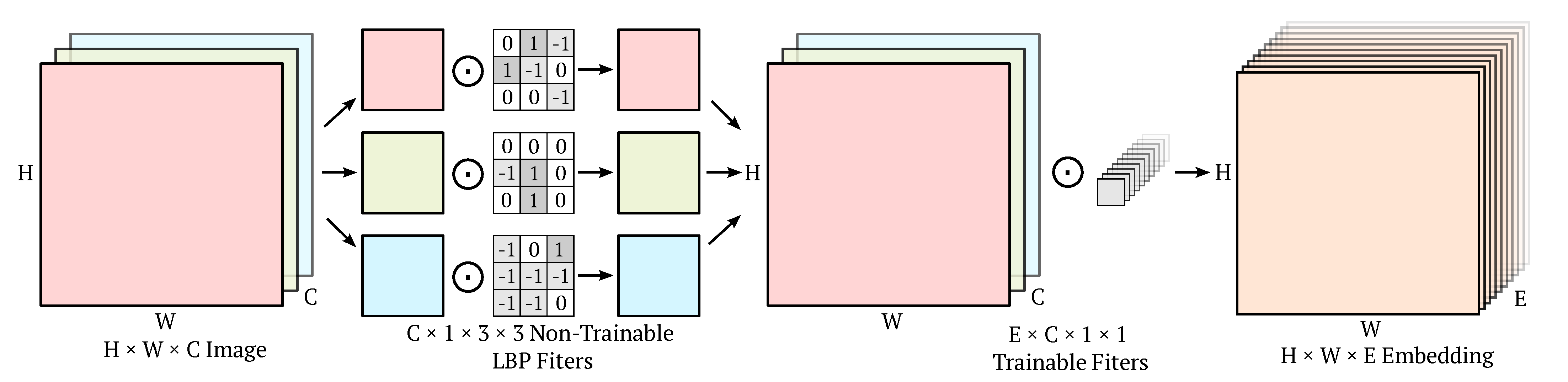
We propose a novel convolutional DSC LBC block that melds DSCs and LBCs in order to reduce the number of operations and trainable parameters. This operation is illustrated in Figure 1 and operates similar to a DSC in that there is first a depthwise convolution, followed by a pointwise convolution. Similar to a DSC, the depthwise convolution stage of a DSC LBC block has filters of size , where a single unique filter is applied to each input channel. The DSC LBC block, however, differs from a DSC in that the depthwise convolution stage uses non-trainable kernels with values initialized from the set , similar to a LBC. This adds sparsity and reduces the total trainable parameters of the DSC LBC block, in contrast to a DSC which uses trainable kernels in the depthwise stage. The initialization of the depthwise kernels in a DSC LBC block occurs in the same manner as described in Section 2.3. When initializing the non-trainable kernels, we use a sparsity of 80% (note that we follow the same convention as the LBCNN authors where the sparsity percentage refers to the percentage of non-zero elements, i.e., sparsity = 100% corresponds to a dense weight tensor [28]) as this level of sparsity achieved the best performance in previous experiments [28]. Finally, the only trainable parameters in a DSC LBC block exist in the pointwise convolution. As a result of this DSC LBC block architecture, we achieve the same computational cost as a DSC of , while using the same number of trainable parameters as a LBC, specifically .
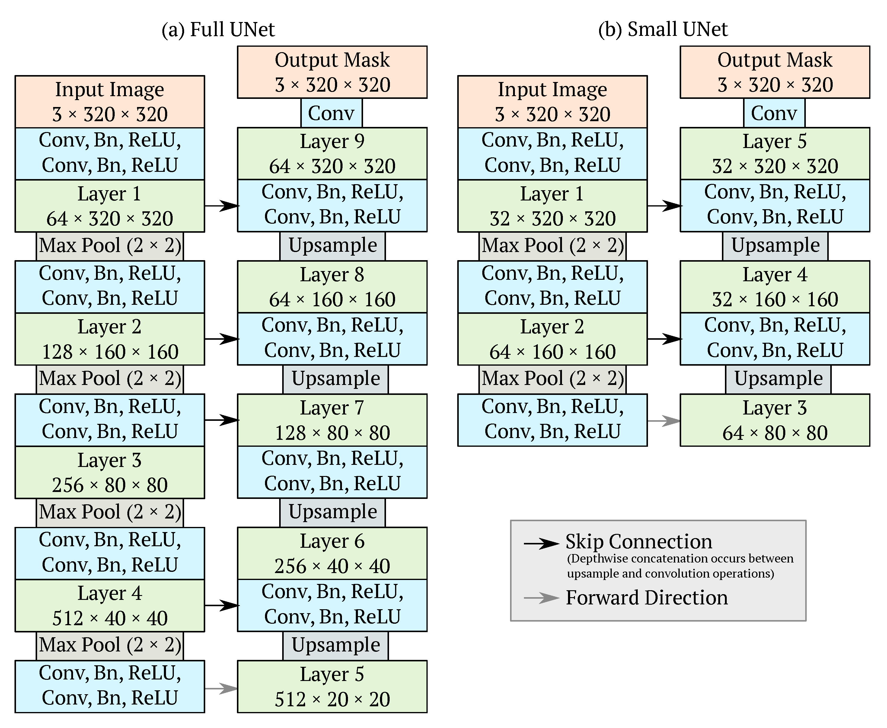
A UNet was chosen as a baseline model due to its simplicity in implementation, widespread use, intuitive interpretation, and success in both performance and generalization ability in previous work [1]. Figure 2a shows the full architecture of a standard UNet as it was originally proposed [22]. For the sake of comparison, various versions of the UNet architecture were created, each with a different convolution operation. Here, the term UNet simply refers to a standard UNet with standard convolution operations, while a DSC UNet replaces standard convolutions with DSCs, and a LBC UNet replaces standard convolutions with LBCs. Finally, we compare these UNet variations to a DSC LBC UNet which replaces standard convolution operations in a UNet with our DSC LBC convolution block. All UNet variations use the same kernel size of .
Previous research has suggested that shallower networks perform better than deeper networks when the dataset of interest is small [44,45]. As the Alberta River Ice Segmentation Dataset is considerably small with only 50 images, we experiment with the size of the UNet with regards to the number of down-sampling and up-sampling layers. The aforementioned UNet variations, which we will now refer to as Full UNets, have four down-sampling and up-sampling layers. We have created similar UNets with only two down-sampling and up-sampling layers and will refer to these as Small UNets (Figure 2b). The Small UNets also differ from the Full UNets in the number of embedding dimensions, or channels used in the intermediate layers. The first two layers of the Full UNets contain 64 and 128 embedding dimensions respectively, while the first two layers of the Small UNets contain 32 and 64 dimensions respectively. This further reduces the memory requirements of these small networks with the goal to improve training and inference efficiency. Finalizing our terminology, the Small UNet uses standard convolutions, while the Small DSC UNet, Small LBC UNet, and Small DSC LBC UNet use DSCs, LBCs, and DSC LBC blocks respectively.
Finally, as we are exploring the performance–latency trade-off for river ice segmentation, we compare the UNet approaches to state-of-the-art MobileNets which are optimized for CPU usage on mobile devises [27]. These networks are built to be fast and efficient, while minimizing any drop in performance. We elect to use use both DeepLabV3 and and the more modern Lite R-ASPP (LR-ASPP) models with a MobileNetV3 backbone. Both these networks have a performance–latency trade-off associated with an output stride; the ratio of the input image size to the output feature map size [26]. A default output stride of 16 was used for DeepLabV3, while a combination of an output stride 8 and 16 was used for low and high level features in the LR-ASPP. These two networks will be referred to as MobileNetV3 (DeepLabV3) and MobileNetV3 (LR-ASPP), respectively.
3.2. Experiments
We run a series of experiments to compare the suite of Full Unets, Small UNets, and MobileNets. The PyTorch library [46] was used to train all models until a stopping criterion had been satisfied. Training was stopped after 30 consecutive training epochs occurred where the validation loss had not reached a new low. After this stopping criterion is triggered, we roll back to the 30th last training epoch where validation loss was at its lowest. This was done in order to mitigate any overfitting that may have occurred during the 30 epochs where validation loss did not decrease. We chose 30 epochs for the stopping criterion as there was significant variation in the validation loss during training due to a small validation set of only 10 images. A batch size of one was used for all experiments in order to maintain consistency and satisfy hardware limitation for the more memory-intensive models. A learning rate of 1 × 10 was used along with a standard cross entropy loss function,
where and are the ground-truth and network output for the ith class of n total classes.
We use an RMSprop optimizer with a weight decay of 1 × 10 and a momentum of 0.9 [47]. Training was conducted on both a GPU and CPU, specifically a Nvidia GeForce GTX 1060 and AMD Ryzen 5 2600 Six-Core Processor respectively. After every three training iterations, a validation step is performed in where the loss function and other evaluation metrics are evaluated for all 10 validation images. This procedure allows for further insight regarding over-fitting and how fast the loss function of validation predictions decreases during training.
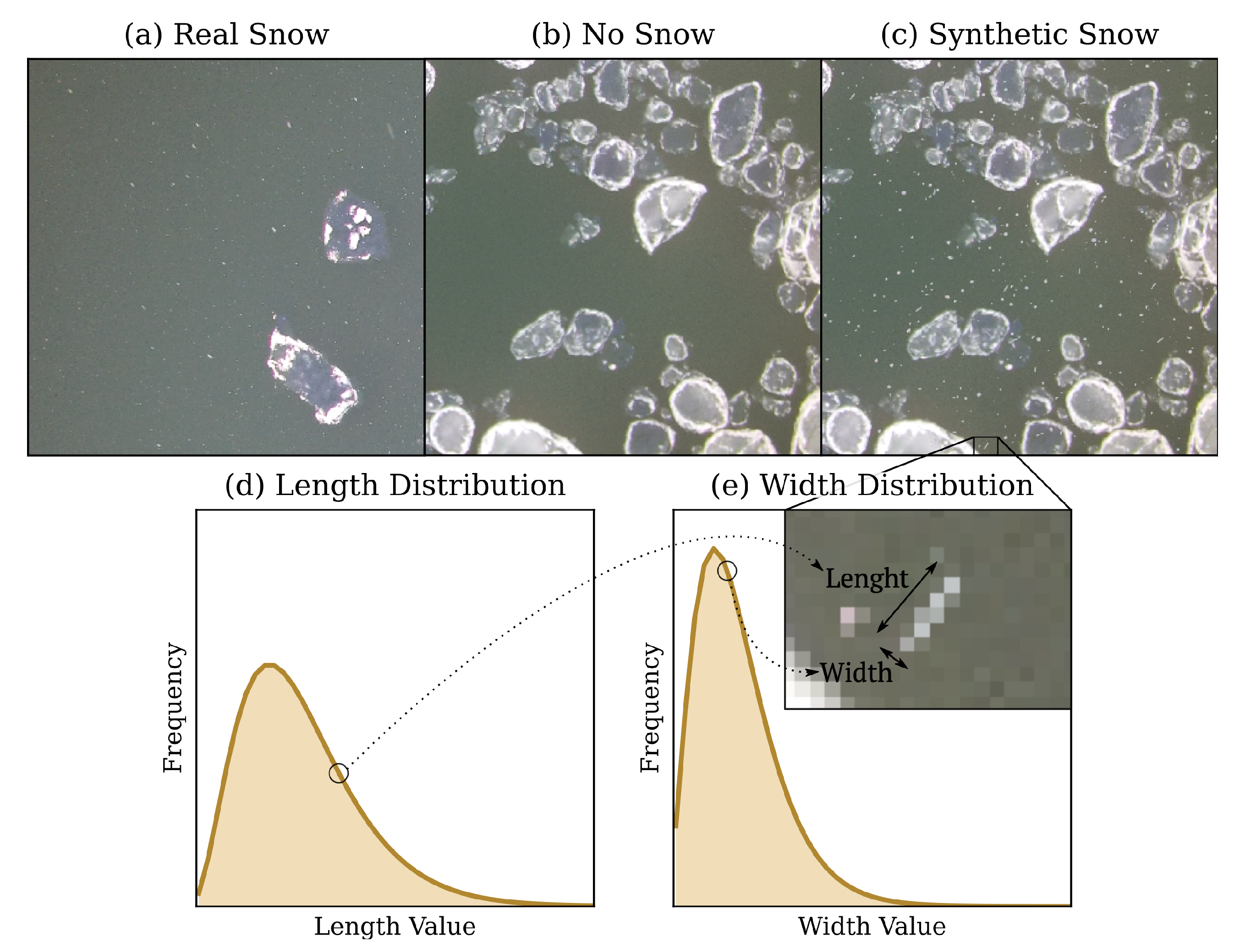
After the suite of UNets and MobileNets have been compared on the Alberta River Ice Segmentation Dataset, we explore the ability of these networks to generalize by adding synthetic snow to a varying number of images in the training and test sets. We evaluate the results of these tests with the non-contaminated ground truth to obtain quantitative results to supplement the qualitative results mentioned in previous work [1]. The synthetic snow was designed by observing UAV footage obtained during a real snowfall [43] (Figure 3a), and was added using the OpenCV library [48] (Figure 3c). The snow observed in the UAV footage has either a point-like or streak-like appearance, as seen in Figure 3a. As a result, a line in OpenCV was used to simulate snow where the length and the width of the lines were sampled from a gamma distribution. If the length and width of the line are similar, the snow appears point-like, while if the length is larger than the width, the snow appears streak-like (Figure 3d,e). A gamma distribution was chosen since the majority of snowflakes are far from the camera and therefore appear smaller, while there are fewer snowflakes near the camera that appear larger. The distribution for the length of the line was sampled from a gamma distribution with a slightly higher mean and standard deviation than the distribution used to sample the width of the line resulting in some streak-like snow. The slant and the colour of the line was chosen from a uniform distribution, where the red, green, and blue colour channels were sampled in the range of 190 to 210 to give the snowflakes a varying greyish white colour.
Finally, we attempt to obtain a better understanding of how model factors such as trainable parameters, multiply–add operations, and memory usage in a model affect the latency during training and inference. We first measure training time over three training epochs for all models on a GPU and CPU to see how fast the various architectures train. Then, the best models from this analysis are compared with respect to the time required to reach a specific metric threshold. This comparison will give a more practical idea of which model is most appropriate to achieve good results when training in a resource and time constrained setting. Then, we finish by measuring the inference time over 10 images for all models on a GPU and a CPU to see how fast river ice images can be evaluated in practice once a model in trained.
4. Results and Discussion
4.1. Metrics
Mean Pixel Accuracy () and Mean Intersect over Union () are the two metrics used to evaluate the performance of the segmentation models.
- Mean Pixel Accuracy is simply the ratio of correctly classified pixels to total labelled pixels per class, averaged over the total number of classes. For k classes, Mean Pixel Accuracy can be calculated bywhere is the total number of pixels both classified and labelled as class j, and is the total number of pixels labelled as class j.
- Mean Intersect over Union is the ratio of the intersection of the predicted segmentation with the ground truth to the union of the predicted segmentation with the ground truth.where k is the number of classes, is the total number of pixels both classified and labelled as class j, is the number of pixels labelled as class i but classified as class j, and is the total number of pixels labelled as class j but classified as class i.
Both and can be expressed as a percentage from 0 to 100, where higher numbers indicate better performance.
4.2. Model Comparison
Table 1 shows a comparison of the various models tested with respect to the evaluation metrics on the test set, the number of total and trainable parameters in the model, the number of multiply–add operations in a pass of the model, and the memory usage of the model. The metrics were calculated by training three instances of each model, saving the respective model weights at the stopping epoch determined during training (Section 3.2), evaluating the models on the test set, and averaging the three results for each model. Memory usage and Mult-Add operations were calculated according to one image passed through the model. Note that it is not expected for the number of parameters and the memory usage of the various models to necessarily correlate. The memory required by the model is a function of both the number of parameters as well as the size of the feature maps at each layer. For a more direct comparison to previous results of UNet on the Alberta River Ice Segmentation Dataset, see the Appendix A. Due to our experiment structure we elect to use a validation and test set, rather than a single test set, as well as more general metric reporting.
When comparing the models within Table 1, the first observation that can be made with respect to evaluation metrics is that the Small UNet variants outperform their Full UNet equivalents. For example, Small UNet outperforms Full UNet, Small DSC UNet outperforms Full DSC UNet, and so on. This gives credibility to the notion that shallower networks outperform deeper networks on smaller datasets.
The Small UNet achieved the highest and results, while the Small DSC LBC UNet used the lowest number of trainable parameters and Mult-Add operations. The Small DSC LBC UNet also had the second smallest memory footprint, second only to MobileNetV3 (LR-ASPP). When comparing the Small DSC LBC UNet to the Full UNet, the Small DSC LBC UNet has a that is virtually the same, only 0.6% higher, but with 99.9% less trainable parameters, 99.0% less Mult-Add operations, and 69.8% less memory usage. When comparing the Small DSC LBC UNet to the best performing Small UNet, the Small DSC LBC UNet has a that is 1.5% lower; however, is still has 94.9% less trainable parameters, 92.3% less Mult-Add operations, and 25.1% less memory usage. Finally, when comparing the Small DSC LBC UNet to MobileNetV3 (LR-ASPP), although the Small DSC LBC UNet uses 51.8% more memory, it uses 23% less Mult-Adds, has 99.6% less trainable parameters, and has a that is 7.7% higher.
The metrics reported in Table 1 were compared to metrics calculated using models trained with data augmentation; specifically random crops from a full-resolution image with random vertical and horizontal flipping. This allows for the exploration of two concepts, namely the effect of the relatively small size of the Alberta River Ice Segmentation Dataset, and the effect of the reduction in resolution from the down-sampling of the main training set. It was found that the data augmentation did not meaningfully improve the results, indicating two things. First, the size of the training set is sufficient without augmentation, likely due to the simple nature of the dataset, in that few images are required to encapsulate the limited variation of the river ice classes. Second, although the down-sampling described in Section 2.5 likely removes fine texture, this fine texture is not critical in discrimination between frazil ice, anchor ice, and water.
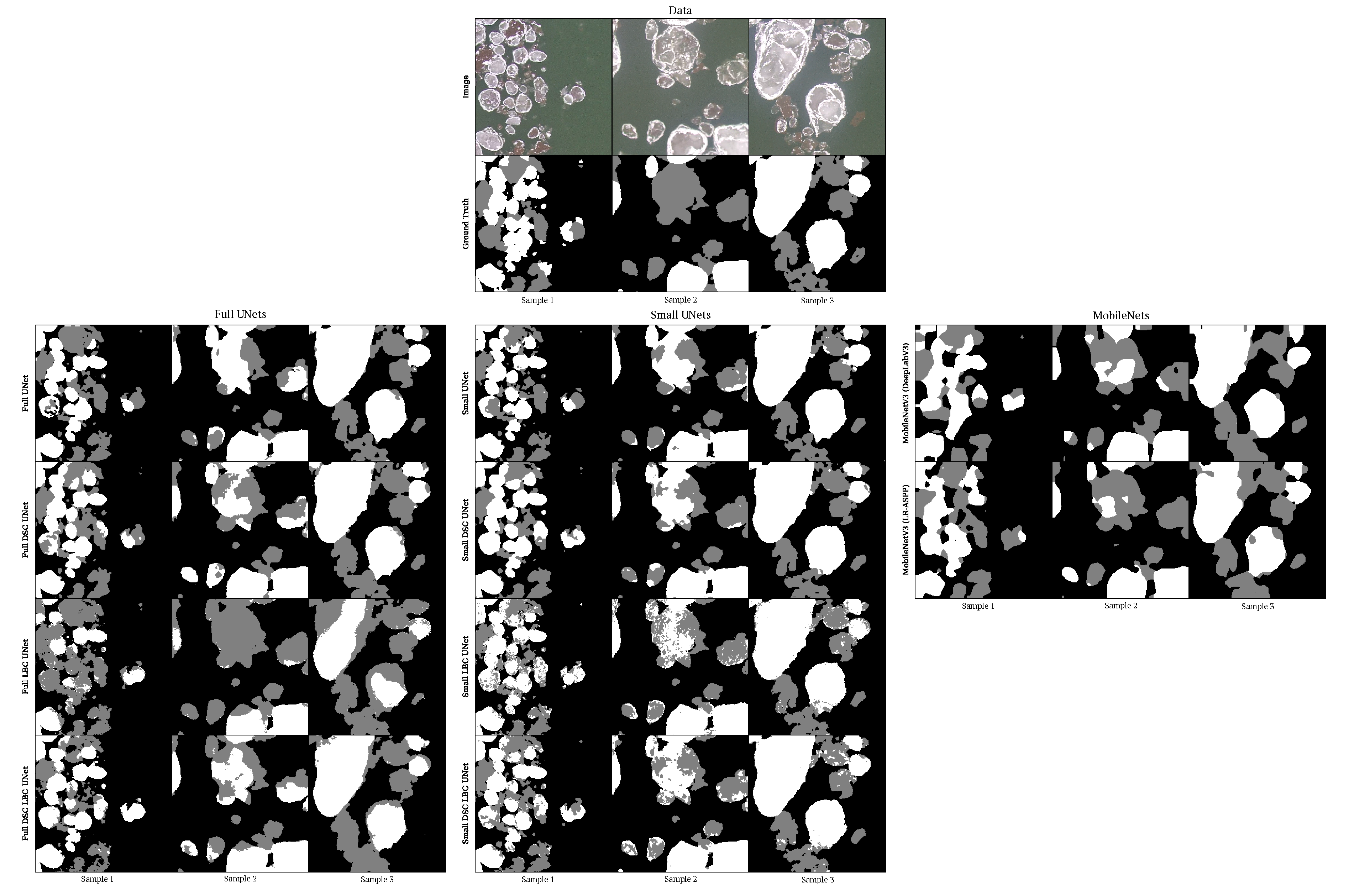
Figure 4 shows model predictions on three test images using model weights saved at the stopping epoch determined during training. When looking at the predicted segmentation outputs, an obvious observation is that the MobileNets have a blobby nature to their segmentation predictions where edges do not have fine detail and smaller ice pans are unnoticed or combined into larger predictions. This nature of MobileNets is acknowledged by the authors and is attributed a larger output stride which allows for parameter saving but reduces the resolution of the predicted masks [26].
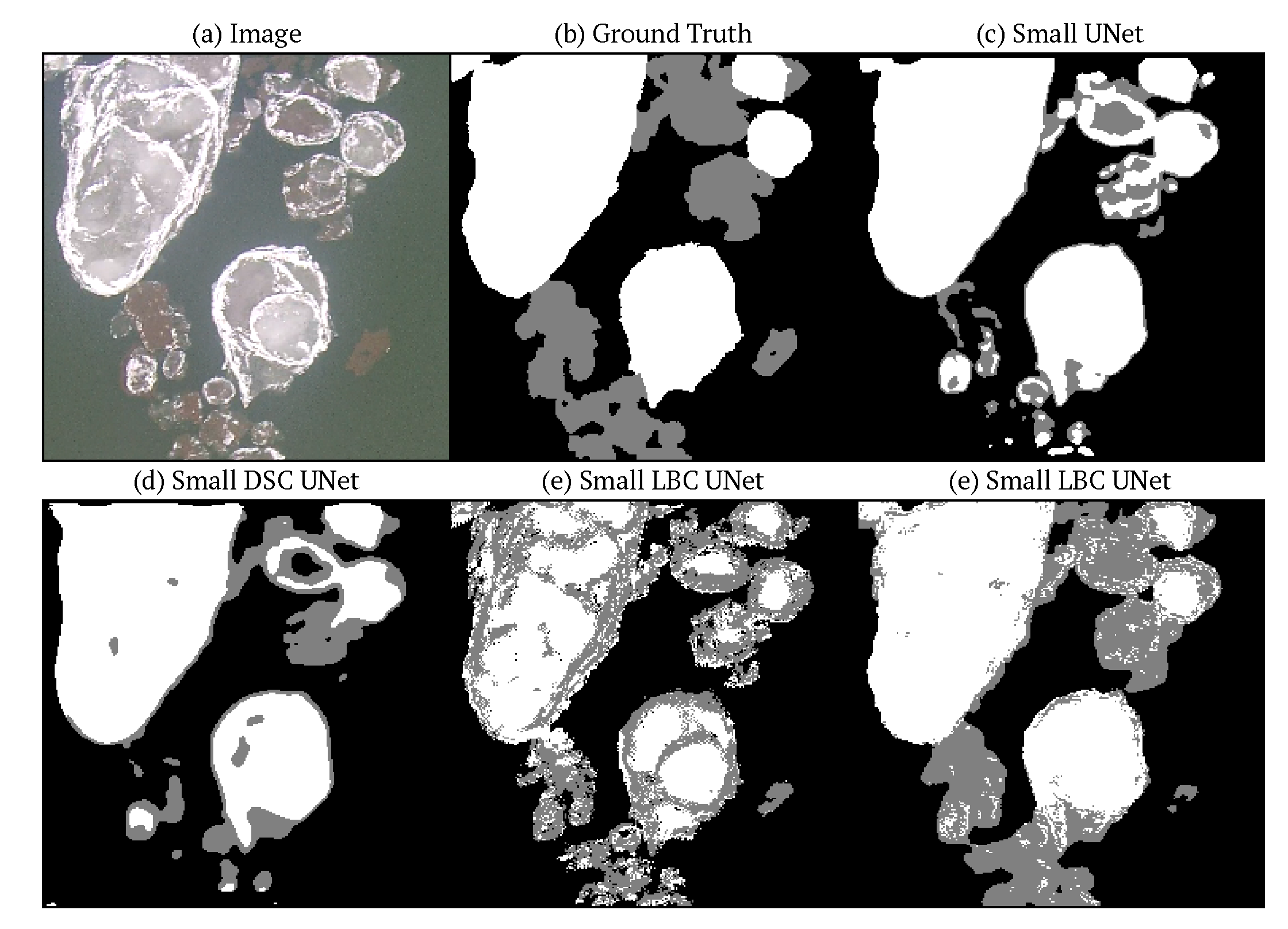
Another observation can be made regarding the LBC portion of the networks which can be seen most clearly in the Small LBC UNet of Figure 4 and even more so in the Small LBC UNet of Figure 5. The LBC component of the networks results in a noisy pixelated appearance of the predicted masks, especially around the boarders of ice pans. The pixilated artifacts are still present, but to lesser extent, in the Small DSC LBC UNet and appear to be reduced with more training. These artifacts are likely due to the sparse binary nature of the LBP filters that propagate through the convolutions early in training. As training progresses, the convolutions are able to account for the sparsity and reduce the pixelated appearance of the predictions. Additionally, this artifact is not as obvious in the Full LBC UNet likely due to the deeper architecture, allowing for more superposition and smoothing of the sparse kernels, limiting the ability for the sparsity to propagate to the predictions early in training. In order to avoid this noise in shallower LBC networks, various post processing techniques could be done including simple smoothing using a Gaussian filter, or the use of a conditional random field (CRF) with an emphasis on pixel proximity to smooth the prediction within an ice pan [49]. Similarly, CRF post-processing could also be applied to the other models including the MobileNets, though for the MobileNets it would be beneficial for the CRF to have an emphasis on pixel intensity to sharpen the smooth edges of the predictions.
Finally, a comparison can be made between the predictions of the Full and Small UNet variations. The Small UNets appear to contain more noise within individual ice pans, while the Full UNets have little variation in class prediction within an individual pan. This can be attributed to the increased down-sampling that occurs within the Full UNets. As down-sampling continues, noise within feature maps get smoothed out and the network learns to value the up-sampled feature maps where the noise is no longer present. Although the smooth predictions appear more realistic, the actual class prediction of the smooth masks are not always correct, which is reflected in the and scores.
4.3. Training Curves and Generalization Ability
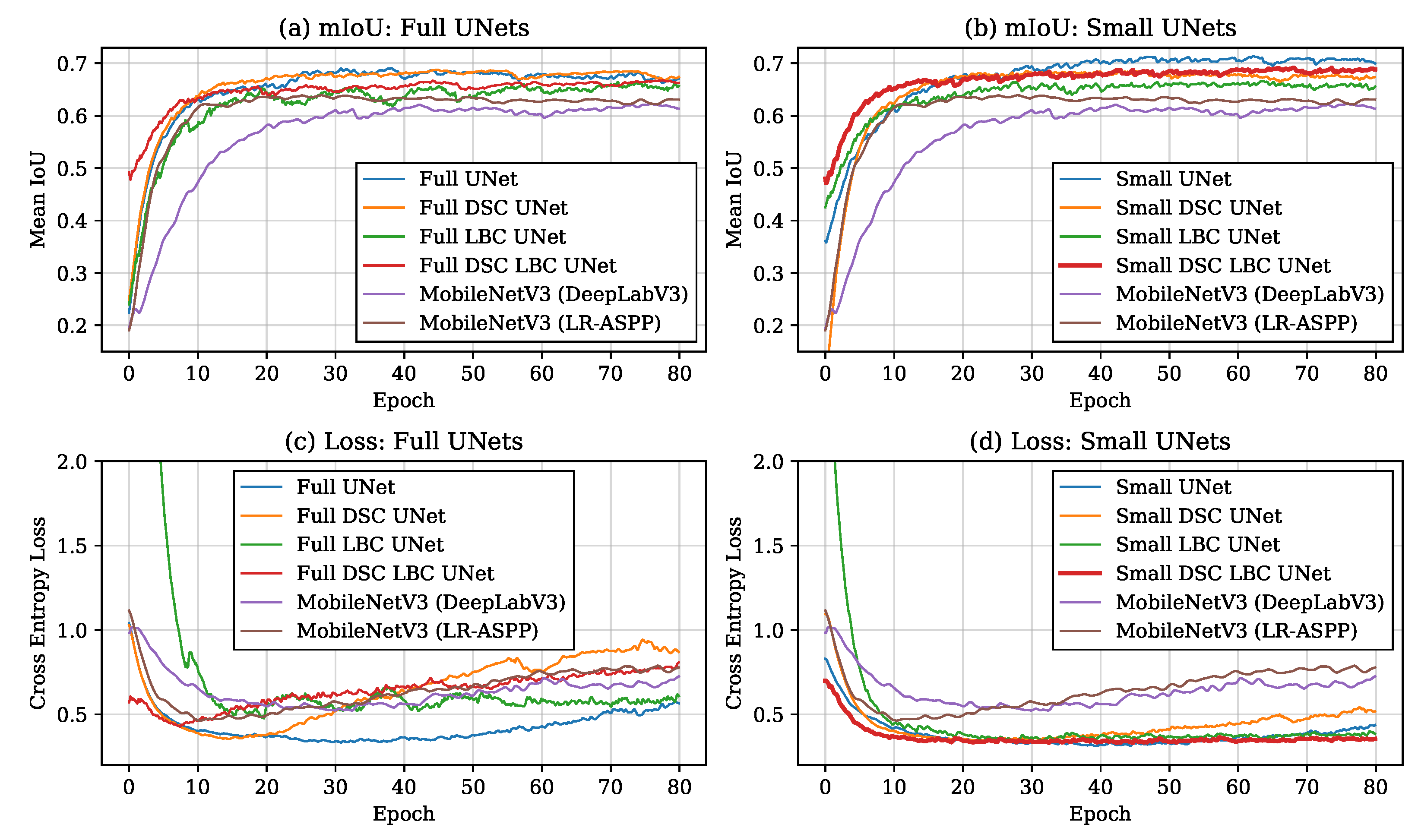
Analyzing the and cross entropy loss of the validation set during training can give insight into the speed of training on an epoch-per-epoch basis, as well as any overfitting that may be occurring. Figure 6 shows the and cross entropy loss of the validation set during 80 epochs of training. It can be seen in Figure 6a,b, that certain models require a fewer number of training iterations in order to reach a given value. In particular, the Small DSC LBC UNet requires the lowest number of training iterations to reach high scores, with the Full DSC LBC UNet, Small DSC UNet, and Small LBC UNet also reaching higher scores considerably sooner than the other models. When comparing these results to Table 1, models with a low number of trainable parameters seem to be the ones that require few iterations to reach high scores. Even still, the combination of DSCs and LBCs, regardless of if the network is small or large, appears to result in high performance early in training.
Figure 5 shows the predictions of the Small UNets on one image of the test set after one epoch of training. The predictions made by the Small DSC LBC UNet are visually much more consistent with the ground truth than the other models at this early stage of training, showing consistency with the training curves of Figure 6. Taking a closer look at Figure 5, there is a key difference between how the Small UNet, Small DSC UNet, and Small LBC UNet learn early in training. The Small UNet and Small DSC UNet are similar in that they appear to focus on pixel intensity in the early stages of training. The upturned bright edges of the anchor ice often often mistaken for the light frazil ice, and the dark interior of the anchor ice is often mistaken for water. On the other hand, the Small LBC UNet tends to focus more on texture in the early stages of training. The rough upturned edges of either ice class are categorized to be anchor ice, while the smooth interiors of the ice pans of either class are categorized as frazil ice. This behaviour of the Small LBC UNet to focus on texture is understandable as the local binary patterns in the kernels are designed to be texture descriptors. The contrasting behaviours of the Small DSC and LBC UNets likely aids in the performance of the Small DSC LBC UNet early in training as it does not appear to make either of the early-training mistakes of the DSC or LBC networks previously mentioned.
It is also important to mention the behaviour of the cross entropy loss of the validation set during training. It can be seen in Figure 6c that validation loss of the Full UNets and MobileNets eventually increases later in training: a sign of overfitting. When contrasting Figure 6a,c, we see that although cross entropy loss increases significantly, the values decrease only very slightly if at all. This discrepancy is attributed to the discrepancy between the softmax output that is used to calculate cross entropy and the argmax output that is used to calculate and . As training proceeds, results are worsening from the perspective of the loss function due to less confident pixel predictions expressed by lowering softmax values. Due to the logarithmic nature of the cross entropy function, changes in smaller softmax values have a larger effect than changes in larger softmax values. However, once an argmax is applied to the softmax, as long as the lowered softmax values are still larger than those of the other classes, the argmax will still have the same result as when the softmax values were more confident. This leads to similar segmentation predictions and no significant decrease in and scores. Although this disconnect between and cross entropy loss has not caused any negative effects over 80 epochs, over longer training we can expect the errors in the softmax output to leak into the argmax and therefore the visual quality of the predicted masks. Looking at Figure 6d, we see that the Small UNets experience this overfitting effect to a much smaller scale. This effect is almost completely non-existent in the Small DSC LBC UNet, allowing for more training to be done before early stopping is triggered. These results are consistent with beliefs that highly complex networks are prone to overfitting when limited data is available [50].
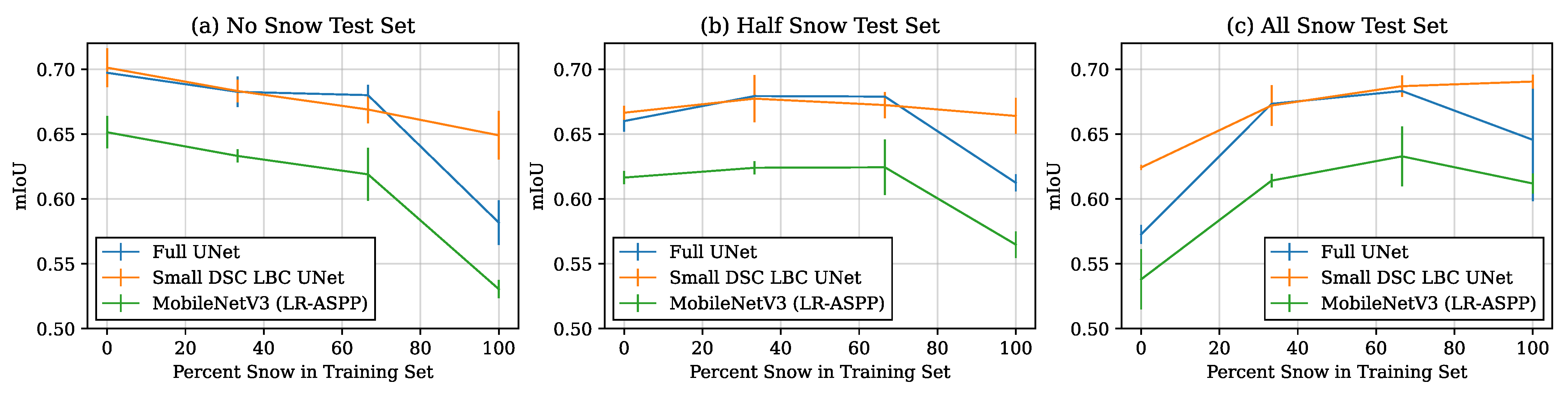
As this overfitting effect does not appear to visually degrade results over the measured epochs, the practical ability for these networks to generalize is still unclear. To obtain more clarity on this topic, and meaningfully test generalization ability as it relates to river ice, we can reference Table 2 which shows the results of the various networks trained on data with no snow but evaluated on data with synthetic snow. We first notice that the general trend of Full UNets outperforming MobileNets, and Small UNets outperforming Full UNets to be consistent with experiments on non-snowy data (Table 1). The results of Table 2, however, differ from Table 1 as the best performing Small network is now the Small DSC LBC UNet and the best performing Full network is the Full DSC LBC UNet, the two of which perform virtually the same. In a perhaps more realistic scenario, some training and testing images may have snow while others do not. Figure 7 shows a variety of scenarios where different amounts of snow are present in the training and testing sets and the associated for three models of interest; the Full UNet, Small DSC LBC UNet, and MobileNetV3 (LR-ASPP). It can be seen that the results of MobileNetV3 (LR-ASPP) under-perform the Full UNet and are highly correlated. The Small DSC LBC UNet performs relatively similar to the Full UNet when the test set has a snow image proportion of or ; however, the Small DSC LBC UNet outperforms the Full UNet significantly in edge cases. These edge cases include high snow during training and no snow during testing, high snow during training and half snow during testing, no snow during training and high snow during testing, and high snow during both training and testing. These results suggest that the DSC LBC convolution mechanism improves a network’s ability to generalize to and from snowy environments; an important feature for a network used in regions where snow is common.
4.4. Performance-Latency Trade-Off
A significant factor affecting the latency of a model is the number of multiply-add operations and memory usage of the model. As seen in Table 1, a trade-off is made between performance, the number of Mult-Add operations and memory usage. The Small UNet has high performance, a high number of Mult-Adds and relatively high memory usage, while MobileNetV3 (LR-ASPP) has slightly lower metric performance but significantly less Mult-Adds and memory requirements. This introduces a performance–latency trade-off where a model can train in much less time but sacrifices some performance. The Small DSC LBC UNet can be considered a good compromise between the performance of the Small UNet and the resource requirements of MobileNetV3 (LR-ASPP).
Table 3 compares both inference frames-per-second (FPS) averaged over the test set and training FPS averaged over three training epochs for the various models on a GPU and CPU. An initial observation reveals that the Small DSC LBC UNet had the fastest training and inference on the GPU, while MobileNetV3 (LR-ASPP) had the fastest training and inference on the CPU. The low number of trainable parameters of the Small DSC LBC UNet may have attributed to its success while training on the GPU, while the CPU specific modifications made to MobileNetV3 (LR-ASPP) can be attributed to its success during CPU training and inference. These CPU-centric modifications, including a hardware-aware network architecture search, exists for MobileNetV3s but not the UNets [27]. Although the Small DSC LBC UNet did not run the fastest on a CPU, it still trained and inferenced significantly faster than the other UNet variations, and considering the performance differences between the Small DSC LBC UNet and MobileNetV3 (LR-ASPP), these results can be considered a favourable trade-off between performance and latency for the Small DSC LBC UNet. On the other hand, although the Small DSC LBC UNet trained the fastest on a GPU, there was no significant improvement over the other models, with an improvement of only 1.59 FPS on average over the worst performing MobileNetV3 (DeepLabV3).
Although it takes MobileNetV3 (LR-ASPP) less time than the Small DSC LBC UNet to complete a training epoch on a CPU, we saw from Figure 6b that the Small DSC LBC UNet requires very few training iterations to achieve good performance. We can therefore frame the idea of run-time slightly differently to make a more fair and practical comparison. Rather than looking at the time to complete n number of training epochs, we can look at the time required to achieve some threshold of performance. Recall from Figure 6 that the training curves are smoothed using an exponential moving average with a smoothing factor of 0.95. When looking at the time to reach a threshold, we also look at a smooth curve as to not stop at an unsustainably high value that is primarily caused by noise.
Table 4 shows the time for the Small DSC LBC UNet and MobileNetV3 (LR-ASPP) to reach various thresholds. We see that the Small DSC LBC UNet outperforms MobileNetV3 (LR-ASPP) for all thresholds. Notably, the largest discrepancy between runtimes occurs at a low (≤48%) and a high (≥64%) , showing that Small DSC LBC UNet is most effective when aiming for either very quick results or very high-performing results. If we consider a of 56% to be satisfactory and a of 64% to be good, then the Small DSC LBC UNet achieves satisfactory results 36% faster than MobileNetV3 (LR-ASPP), and achieves good results 91% faster than MobileNetV3 (LR-ASPP) when trained on a CPU.
5. Conclusions
In this paper we balance the trade-off between performance and latency for the task of river ice segmentation on the Peace River and North Saskatchewan River. We introduce a new convolutional block, the DSC LBC block, and use it to construct a shallow UNet style architecture. The DSC LBC block combines the benefits of depthwise separable convolutions and local binary convolutions to minimize both the number of operations and the number of trainable parameters in a convolution. We find that the DSC LBC convolution adds efficiency and improves a network’s ability to generalize to other domains such as a snowy environment. Our novel architecture has performance on par with UNet, but with 99.9% less trainable parameters, 99% less multiply–add operations, and 69.8% less memory usage, resulting in significantly faster training and inference. When compared to state-of-the-art efficient networks such as LR-ASPP MobleNetV3, our architecture not only achieves a value that is 7.7% higher over extended training, it can achieve satisfactory results ( of 56) 36% faster than LR-ASPP MobleNetV3, a good result ( of 64) 91% faster than LR-ASPP MobleNetV3 on a CPU, and even more impressive results on a GPU. This success attributed to the shallow nature of the architecture, the lightweight nature of DSC LBC convolutions, and the ability for the DSC LBC convolution to focus on both texture and pixel intensity, allowing for better performance early in the training process. These results give promise to real time river ice segmentation in remote regions where limited hardware and computation power is available and winter weather conditions can affect image quality. This can allow for rapid and frequent estimates of mass flux caused by anchor ice rafting, leading to more accurate estimates of annual sediment budgets.
Author Contributions
D.S. and K.A.S. conceptualized and designed the methodology for the study. D.S. completed the algorithm design and experiments. D.S. led the writing of the manuscript, with contributions from K.A.S. All authors have read and agreed to the published version of the manuscript.
Funding
This research was funded by the Natural Sciences and Engineering Research Council of Canada (NSERC).
Data Availability Statement
The data used in this study were made openly available by other authors in IEEE DataPort at doi:10.21227/ebax-1h44 [43].
Acknowledgments
Conflicts of Interest
The authors declare no conflict of interest.
Sample Availability
Samples of the compounds are available from the authors.
Appendix A. Direct Comparison to Previous Work
We compare our results directly to previous work [1] on the Alberta River Ice Segmentation Dataset. We use the same metrics used in previous work and use the same implementation as was shown in the publicly available code [51]. These metrics are pixel accuracy, , mean pixel accuracy , mean intersect over union, , and frequency weighted intersect over union, . and are calculated the same as Equations (6) and (7) respectively, while and are calculated as follows,
where is the total number of pixels both classified and labelled as class j, is the number of pixels labelled as class i but classified as class j, and is the total number of pixels labelled class j. Note that we follow the notation of the previous author by referring to and as recall and precision respectively.
Table A1 shows the Small DSC LBC UNet outperforms the previously tested UNet [1], while MobileNetV3 (LR-ASPP) underperforms relative to the previously tested UNet [1] using the same training and testing set. The training set contains 32 images while the test set contains 18 images. These trends are similar to those observed in Table 1.

Table A1.
Metric comparison of the Small DSC LBC UNet and MobileNetV3 (LR-ASPP) with the UNet tested in previous work using the same training and testing split. Recall and precision for the two ice types correspond to class specific and . Ice + Water recall and precision correspond to and respectively for all classes. The frequency weighted (fw) equivalents for Ice + Water recall and precision correspond to and respectively for all classes.
| Model | Anchor Ice Recall | Frazil Ice Recall | Ice + Water Recall | Ice + Water Recall (fw) |
|---|---|---|---|---|
| Previous UNet [1] | 73.75 | 84.27 | 85.13 | 88.69 |
| Small DSC LBC UNet | 74.18 | 87.28 | 86.84 | 90.57 |
| MobileNetV3 (LR-ASPP) | 77.35 | 80.22 | 84.32 | 86.99 |
| Model | Anchor Ice Precision | Frazil Ice Precision | Ice + Water Precision | Ice + Water Precision (fw) |
| Previous UNet [1] | 54.89 | 71.17 | 73.19 | 81.73 |
| Small DSC LBC UNet | 56.59 | 73.17 | 74.78 | 84.70 |
| MobileNetV3 (LR-ASPP) | 48.50 | 65.82 | 68.29 | 79.54 |
References
- Singh, A.; Kalke, H.; Loewen, M.; Ray, N. River ice segmentation with deep learning. IEEE Trans. Geosci. Remote Sens. 2020, 58, 7570–7579. [Google Scholar] [CrossRef] [Green Version]
- Hicks, F. An Overview of River Ice Problems: CRIPE07 Guest Editorial. Cold Regions Sci. Technol. 2009, 55, 175–185. [Google Scholar] [CrossRef]
- Beltaos, S. Progress in the study and management of river ice jams. Cold Reg. Sci. Technol. 2008, 51, 2–19. [Google Scholar] [CrossRef]
- Kalke, H.; Loewen, M. Support vector machine learning applied to digital images of river ice conditions. Cold Reg. Sci. Technol. 2018, 155, 225–236. [Google Scholar] [CrossRef]
- Peters, D.L.; Prowse, T.D. Regulation effects on the lower Peace River, Canada. Hydrol. Process. 2001, 15, 3181–3194. [Google Scholar] [CrossRef]
- Piesold, K. Fluvial Geomorphology and Sediment Transport Technical Data Report; BC Hydro: Vancouver, BC, Canada, 2011. [Google Scholar]
- Kalke, H.; Loewen, M.; McFarlane, V.; Jasek, M. Observations of anchor ice formation and rafting of sediments. In Proceedings of the 18th Workshop on the Hydraulics of Ice Covered Rivers, Quebec City, QC, Canada, 18–20 August 2015. [Google Scholar]
- Kalke, H.; McFarlane, V.; Schneck, C.; Loewen, M. The transport of sediments by released anchor ice. Cold Reg. Sci. Technol. 2017, 143, 70–80. [Google Scholar] [CrossRef]
- Ansari, S.; Rennie, C.D.; Clark, S.P.; Seidou, O. Application of a Fast Superpixel Segmentation Algorithm in River Ice Classification. In Proceedings of the 20th Workshop on the Hydraulics of Ice Covered Rivers, Ottawa, ON, Canada, 14–16 May 2019. [Google Scholar]
- Zhang, X.; Jin, J.; Lan, Z.; Li, C.; Fan, M.; Wang, Y.; Yu, X.; Zhang, Y. ICENET: A semantic segmentation deep network for river ice by fusing positional and channel-wise attentive features. Remote Sens. 2020, 12, 221. [Google Scholar] [CrossRef] [Green Version]
- Zhang, X.; Zhou, Y.; Jin, J.; Wang, Y.; Fan, M.; Wang, N.; Zhang, Y. ICENETv2: A Fine-Grained River Ice Semantic Segmentation Network Based on UAV Images. Remote Sens. 2021, 13, 633. [Google Scholar] [CrossRef]
- Van Beeck, K.; Tuytelaars, T.; Scarramuza, D.; Goedemé, T. Real-time embedded computer vision on UAVs. In Proceedings of the European Conference on Computer Vision, Munich, Germany, 8–14 September 2018; Springer: Berlin/Heidelberg, Germany, 2018; pp. 3–10. [Google Scholar]
- Yang, X.; Chen, J.; Dang, Y.; Luo, H.; Tang, Y.; Liao, C.; Chen, P.; Cheng, K.T. Fast depth prediction and obstacle avoidance on a monocular drone using probabilistic convolutional neural network. IEEE Trans. Intell. Transp. Syst. 2019, 32, 156–167. [Google Scholar] [CrossRef]
- Jiao, Z.; Zhang, Y.; Xin, J.; Mu, L.; Yi, Y.; Liu, H.; Liu, D. A deep learning based forest fire detection approach using UAV and YOLOv3. In Proceedings of the 2019 1st International Conference on Industrial Artificial Intelligence (IAI), Shenyang, China, 22–26 July 2019; IEEE: Piscataway, NJ, USA, 2019; pp. 1–5. [Google Scholar]
- Yang, Q.; Shi, L.; Han, J.; Yu, J.; Huang, K. A near real-time deep learning approach for detecting rice phenology based on UAV images. Agric. For. Meteorol. 2020, 287, 107938. [Google Scholar] [CrossRef]
- Nagi, A.S.; Kumar, D.; Sola, D.; Scott, K.A. RUF: Effective Sea Ice Floe Segmentation Using End-to-End RES-UNET-CRF with Dual Loss. Remote Sens. 2021, 13, 2460. [Google Scholar] [CrossRef]
- Wagner, P.M.; Hughes, N.; Bourbonnais, P.; Stroeve, J.; Rabenstein, L.; Bhatt, U.; Little, J.; Wiggins, H.; Fleming, A. Sea-ice information and forecast needs for industry maritime stakeholders. Polar Geogr. 2020, 43, 160–187. [Google Scholar] [CrossRef]
- Ansari, S.; Rennie, C.; Seidou, O.; Malenchak, J.; Zare, S. Automated monitoring of river ice processes using shore-based imagery. Cold Reg. Sci. Technol. 2017, 142, 1–16. [Google Scholar] [CrossRef]
- Bharathi, P.; Subashini, P. Texture based color segmentation for infrared river ice images using K-means clustering. In Proceedings of the 2013 International Conference on Signal Processing, Image Processing & Pattern Recognition, Coimbatore, India, 7–8 February 2013; IEEE: Piscataway, NJ, USA, 2013; pp. 298–302. [Google Scholar]
- Kalke, H.; Loewen, M. Predicting surface ice concentration using machine learning. In Proceedings of the 19th Workshop on the Hydraulics of Ice Covered Rivers, Whitehorse, YT, Canada, 9–12 July 2017. [Google Scholar]
- Chen, L.C.; Zhu, Y.; Papandreou, G.; Schroff, F.; Adam, H. Encoder-decoder with atrous separable convolution for semantic image segmentation. In Proceedings of the European conference on computer vision (ECCV), Munich, Germany, 8–14 September 2018; pp. 801–818. [Google Scholar]
- Ronneberger, O.; Fischer, P.; Brox, T. U-net: Convolutional networks for biomedical image segmentation. In Proceedings of the International Conference on Medical Image Computing and Computer-Assisted Intervention, Munich, Germany, 5–9 October 2015; Springer: Berlin/Heidelberg, Germany, 2015; pp. 234–241. [Google Scholar]
- Howard, A.G.; Zhu, M.; Chen, B.; Kalenichenko, D.; Wang, W.; Weyand, T.; Andreetto, M.; Adam, H. Mobilenets: Efficient convolutional neural networks for mobile vision applications. arXiv 2017, arXiv:1704.04861. [Google Scholar]
- Chollet, F. Xception: Deep Learning With Depthwise Separable Convolutions. In Proceedings of the IEEE Conference on Computer Vision and Pattern Recognition (CVPR), Honolulu, HI, USA, 21–26 July 2017. [Google Scholar]
- Zhang, X.; Zhou, X.; Lin, M.; Sun, J. Shufflenet: An extremely efficient convolutional neural network for mobile devices. In Proceedings of the IEEE Conference on Computer Vision and Pattern Recognition, Salt Lake City, UT, USA, 18–23 June 2018; pp. 6848–6856. [Google Scholar]
- Sandler, M.; Howard, A.; Zhu, M.; Zhmoginov, A.; Chen, L.C. Mobilenetv2: Inverted residuals and linear bottlenecks. In Proceedings of the IEEE Conference on Computer Vision and Pattern Recognition, Salt Lake City, UT, USA, 18–23 June 2018; pp. 4510–4520. [Google Scholar]
- Howard, A.; Sandler, M.; Chu, G.; Chen, L.C.; Chen, B.; Tan, M.; Wang, W.; Zhu, Y.; Pang, R.; Vasudevan, V.; et al. Searching for mobilenetv3. In Proceedings of the IEEE/CVF International Conference on Computer Vision, Seoul, Korea, 27–28 October 2019; pp. 1314–1324. [Google Scholar]
- Juefei-Xu, F.; Naresh Boddeti, V.; Savvides, M. Local binary convolutional neural networks. In Proceedings of the IEEE Conference on Computer Vision and Pattern Recognition, Honolulu, HI, USA, 21–26 July 2017; pp. 19–28. [Google Scholar]
- Ojala, T.; Pietikainen, M.; Maenpaa, T. Multiresolution gray-scale and rotation invariant texture classification with local binary patterns. IEEE Trans. Pattern Anal. Mach. Intell. 2002, 24, 971–987. [Google Scholar] [CrossRef]
- Ahonen, T.; Hadid, A.; Pietikainen, M. Face description with local binary patterns: Application to face recognition. IEEE Trans. Pattern Anal. Mach. Intell. 2006, 28, 2037–2041. [Google Scholar] [CrossRef] [PubMed]
- Tan, M.; Chen, B.; Pang, R.; Vasudevan, V.; Sandler, M.; Howard, A.; Le, Q.V. Mnasnet: Platform-aware neural architecture search for mobile. In Proceedings of the IEEE/CVF Conference on Computer Vision and Pattern Recognition, Long Beach, CA, USA, 15–20 June 2019; pp. 2820–2828. [Google Scholar]
- Chen, L.C.; Papandreou, G.; Schroff, F.; Adam, H. Rethinking atrous convolution for semantic image segmentation. arXiv 2017, arXiv:1706.05587. [Google Scholar]
- Chen, L.C.; Papandreou, G.; Kokkinos, I.; Murphy, K.; Yuille, A.L. Deeplab: Semantic image segmentation with deep convolutional nets, atrous convolution, and fully connected crfs. IEEE Trans. Pattern Anal. Mach. Intell. 2017, 40, 834–848. [Google Scholar] [CrossRef] [Green Version]
- Hu, J.; Shen, L.; Sun, G. Squeeze-and-excitation networks. In Proceedings of the IEEE Conference on Computer Vision and Pattern Recognition, Salt Lake City, UT, USA, 18–23 June 2018; pp. 7132–7141. [Google Scholar]
- Paszke, A.; Chaurasia, A.; Kim, S.; Culurciello, E. Enet: A deep neural network architecture for real-time semantic segmentation. arXiv 2016, arXiv:1606.02147. [Google Scholar]
- Yu, C.; Wang, J.; Peng, C.; Gao, C.; Yu, G.; Sang, N. Bisenet: Bilateral segmentation network for real-time semantic segmentation. In Proceedings of the European Conference on Computer Vision (ECCV), Munich, Germany, 8–14 September 2018; pp. 325–341. [Google Scholar]
- Li, H.; Xiong, P.; Fan, H.; Sun, J. Dfanet: Deep feature aggregation for real-time semantic segmentation. In Proceedings of the IEEE/CVF Conference on Computer Vision and Pattern Recognition, Long Beach, CA, USA, 16–17 June 2019; pp. 9522–9531. [Google Scholar]
- Chen, W.; Gong, X.; Liu, X.; Zhang, Q.; Li, Y.; Wang, Z. Fasterseg: Searching for faster real-time semantic segmentation. arXiv 2019, arXiv:1912.10917. [Google Scholar]
- Jacob, B.; Kligys, S.; Chen, B.; Zhu, M.; Tang, M.; Howard, A.; Adam, H.; Kalenichenko, D. Quantization and training of neural networks for efficient integer-arithmetic-only inference. In Proceedings of the IEEE Conference on Computer Vision and Pattern Recognition, Salt Lake City, UT, USA, 18–23 June 2018; pp. 2704–2713. [Google Scholar]
- Krishnamoorthi, R. Quantizing deep convolutional networks for efficient inference: A whitepaper. arXiv 2018, arXiv:1806.08342. [Google Scholar]
- Frankle, J.; Carbin, M. The lottery ticket hypothesis: Finding sparse, trainable neural networks. arXiv 2018, arXiv:1803.03635. [Google Scholar]
- Hinton, G.; Vinyals, O.; Dean, J. Distilling the knowledge in a neural network. arXiv 2015, arXiv:1503.02531. [Google Scholar]
- Singh, A.; Kalke, H.; Loewen, M.; Ray, N. Alberta River Ice Segmentation Dataset; IEEE Dataport: New York, NY, USA, 2019. [Google Scholar] [CrossRef]
- Schindler, A.; Lidy, T.; Rauber, A. Comparing Shallow versus Deep Neural Network Architectures for Automatic Music Genre Classification. In Proceedings of the FMT, St. Polten, Austria, 23–24 November 2016; pp. 17–21. [Google Scholar]
- Pasupa, K.; Sunhem, W. A comparison between shallow and deep architecture classifiers on small dataset. In Proceedings of the 2016 8th International Conference on Information Technology and Electrical Engineering (ICITEE), Yogyakarta, Indonesia, 5–6 October 2016; IEEE: Piscataway, NJ, USA, 2016; pp. 1–6. [Google Scholar]
- Paszke, A.; Gross, S.; Massa, F.; Lerer, A.; Bradbury, J.; Chanan, G.; Killeen, T.; Lin, Z.; Gimelshein, N.; Antiga, L.; et al. Pytorch: An imperative style, high-performance deep learning library. Adv. Neural Inf. Process. Syst. 2019, 32, 8026–8037. [Google Scholar]
- Tieleman, T.; Hinton, G. Divide the gradient by a running average of its recent magnitude. COURSERA Neural Netw. Mach. Learn. 2012, 42, 26–31. [Google Scholar]
- Bradski, G. Dr. Dobb’s Journal of Software Tools; The OpenCV Library’: Hilton Head, SC, USA, 2000. [Google Scholar]
- Krähenbühl, P.; Koltun, V. Efficient inference in fully connected crfs with gaussian edge potentials. In Advances in Neural Information Processing Systems 24 (NIPS 2011), Proceedings of the 24th International Conference on Neural Information Processing Systems, Red Hook, NY, USA, 12–15 December 2011; Curran Associates Inc.: Red Hook, NY, USA, 2011; pp. 109–117. [Google Scholar] [CrossRef]
- Srivastava, N.; Hinton, G.; Krizhevsky, A.; Sutskever, I.; Salakhutdinov, R. Dropout: A simple way to prevent neural networks from overfitting. J. Mach. Learn. Res. 2014, 15, 1929–1958. [Google Scholar]
- Singh, A. River_ice_segmentation. In GitHub Repository; GitHub: San Francisco, CA, USA, 2021. [Google Scholar]
Figure 1.
DSC LBC convolution block used to replace a standard convolution. A given convolution operation can be considered to have X filters of size K × K × Y where X is the number of output channels, Y is the number of input channels divided by the number of convolution groups, and K is the width and the height the kernel. A DSC LBC convolution replaces the trainable depthwise filters of a depthwise separable convolution [24] with sparse, non-trainable filters inspired by local binary patterns [28]. Note that there is only one distinct non-trainable binary filter convolved with each input channel in the first stage of the DSC LBC convolution block.

Figure 2.
Original UNet architecture shown in (a) [22], and smaller UNet architecture shown in (b) with only two down-sampling stages. If the Conv operation in the blue boxes is a standard convolution, the networks are referred to as Full and Small UNets. If the Conv operation is a DSC operation, the networks are referred to as Full and Small DSC UNets. If the Conv operation is a LBC operation, the networks are referred to as Full and Small LBC UNets. If the Conv operation is a DSC LBC operation (Figure 1), the networks are referred to as Full and Small DSC LBC UNets.

Figure 3.
Examples from the Alberta River Ice Segmentation Dataset [43] taken while it is snowing (a), while it is not snowing (b), and with synthetic snow added to an image which originally had no snow (c). An example of a synthetic streak-like snowflake is shown with its length and width sampled from gamma distributions for length (d) and width (e). The distribution for length (d) can be seen to have a larger mean and standard deviation than the distribution for width, forcing some streak-like snow as shown in the zoomed in square. Note that snow can be seen better when zoomed in.

Figure 4.
Segmentation results on three images from the test set. Model weights for the various models were chosen based on a stopping criterion during training (see Section 3.2). The original image and ground-truth are shown at the top, the Full UNet variations are shown on the left, the Small UNet variations are shown in the centre, and the two MobileNet variations are shown on the right. Water, anchor ice, and frazil ice are coloured in black, gray, and white, respectively. Note that details in the images and segmentation predictions can be best seen when zoomed in.

Figure 5.
Comparison of predictions after one epoch of training on the suite of Small UNets. The mean IoU for the Small UNet, Small DSC UNet, Small LBC UNet and Small DSC LBC UNet are 65.9, 67.2, 56.7, and 78.7, respectively. The mean pixel accuracy for the Small UNet, Small DSC UNet, Small LBC UNet and Small DSC LBC UNet are 75.0, 76.0, 69.2, and 88.8 respectively. Note that detail can be more easily observed when zoomed in.

Figure 6.
Mean IoU of the validation set after 80 training epochs is shown for the Full UNets (a) and Small UNets (b). Cross entropy loss for the validation set is also shown over 80 epochs for the Full UNets (c) and Small UNets (d). Note that the MobileNets are shown in all chats for the sake of comparison. The data in all of the charts has an exponential moving average applied with a smoothing factor or 0.95 to filter noise caused by a small validation set.

Figure 7.
mIoU results for a Full UNet, Small DSC LBC UNet, and MobileNetV3 (LR-ASPP) for varying numbers of images with snow in the training and test sets. Training sets had either 0/30, 10/30, 20/30, or 30/30 of the images containing snow, while the test set had either 0/10 (a), 5/10 (b), or 10/10 (c) of the images containing snow. Three instances of each model were trained under each scenario and their mean value was used with the standard deviation shown by the error bar.

Table 1.
Metrics, number of parameters, number of multiply–add operations and memory usage in the tested networks. Metrics were calculated by training three instances of each model, evaluating them on an external test set using weights saved at the stopping criterion, and averaging the three results. Memory and Mult-Adds were calculated using an input size of . Numbers in bold represent the highest metric or lowest number of parameters/operations/memory of the models tested. Small DSC LBC UNet is in bold as it shows a healthy trade-off between high performance metrics and low parameters/operations/memory.
| Model | mIoU | mPA | Total Params | Trainable Params | Mult-Adds | Memory |
|---|---|---|---|---|---|---|
| Full UNet | 69.7 | 82.7 | 17,267,523 | 17,267,523 | 62,764 M | 1542 MB |
| Full DSC UNet | 69.7 | 82.9 | 1,983,713 | 1,983,713 | 7717 M | 2242 MB |
| Full LBC UNet | 67.7 | 82.2 | 16,498,842 | 794,697 | 71,048 M | 1164 MB |
| Full DSC LBC UNet | 69.1 | 82.7 | 821,220 | 794,697 | 3402 M | 1104 MB |
| Small UNet | 71.2 | 85.0 | 260,451 | 260,451 | 8237 M | 622 MB |
| Small DSC UNet | 70.4 | 84.3 | 35,777 | 35,777 | 1123 M | 936 MB |
| Small LBC UNet | 69.7 | 83.8 | 253,050 | 13,353 | 9479 M | 468 MB |
| Small DSC LBC UNet | 70.1 | 83.5 | 16,260 | 13,353 | 637 M | 466 MB |
| MobileNetV3 (DeepLabV3) | 63.7 | 78.5 | 11,020,851 | 11,020,851 | 3898 M | 589 MB |
| MobileNetV3 (LR-ASPP) | 65.1 | 80.0 | 3,218,478 | 3,218,478 | 826 M | 307 MB |
Table 2.
mIoU and mPA scores on the test set corrupted with snow noise. Models were trained on the training set without snow noise. Numbers in bold highlight the best scores while the Small DSC LBC UNet is in bold as it is the model of interest.
Table 2.
mIoU and mPA scores on the test set corrupted with snow noise. Models were trained on the training set without snow noise. Numbers in bold highlight the best scores while the Small DSC LBC UNet is in bold as it is the model of interest.
| Model | mIoU | mPA |
|---|---|---|
| Full UNet | 58.1 | 71.0 |
| Full DSC UNet | 57.6 | 72.0 |
| Full LBC UNet | 56.5 | 70.5 |
| Full DSC LBC UNet | 62.9 | 76.8 |
| Small UNet | 58.9 | 71.0 |
| Small DSC UNet | 59.1 | 71.1 |
| Small LBC UNet | 57.0 | 71.7 |
| Small DSC LBC UNet | 62.4 | 76.1 |
| MobileNetV3 (DeepLabV3) | 49.7 | 62.3 |
| MobileNetV3 (LR-ASPP) | 53.0 | 62.8 |
Table 3.
Training and inference runtime measured in frames-per-second (FPS) on a Nvidia GeForce GTX 1060 GPU and AMD Ryzen 5 2600 Six-Core CPU. Images of size were used during training and inference where the training FPS was averaged over three epochs and the inference FPS was averaged over the test set of 10 images. Bold numbers indicate the fastest runtime, while the Small DSC LBC UNet is in bold as it is the model of interest.
| Model | GPU Train (FPS) | GPU Inference (FPS) | CPU Train (FPS) | CPU Inference (FPS) |
|---|---|---|---|---|
| Full UNet | 10.59 | 21.69 | 0.72 | 1.29 |
| Full DSC UNet | 10.25 | 21.79 | 1.36 | 2.30 |
| Full LBC UNet | 11.17 | 21.83 | 0.92 | 1.18 |
| Full DSC LBC UNet | 16.07 | 21.98 | 2.23 | 2.99 |
| Small UNet | 18.82 | 21.88 | 3.21 | 4.83 |
| Small DSC UNet | 18.00 | 21.93 | 3.71 | 5.62 |
| Small LBC UNet | 19.35 | 22.07 | 3.94 | 4.69 |
| Small DSC LBC UNet | 19.57 | 22.47 | 5.78 | 6.54 |
| MobileNetV3 (DeepLabV3) | 13.27 | 20.88 | 3.27 | 8.00 |
| MobileNetV3 (LR-ASPP) | 15.54 | 21.19 | 6.32 | 12.35 |
Table 4.
Time in seconds for Small DSC LBC UNet and MobineNetV3 (LR-ASPP) to reach various mIoU thresholds on an AMD Ryzen 5 2600 Six-Core CPU.
Table 4.
Time in seconds for Small DSC LBC UNet and MobineNetV3 (LR-ASPP) to reach various mIoU thresholds on an AMD Ryzen 5 2600 Six-Core CPU.
| mIoU Threshold | Small DSC LBC UNet Time | MobileNetV3 (LR-ASPP) Time |
|---|---|---|
| 48 | 2.16 s | 18.05 s |
| 52 | 15.57 s | 24.70 s |
| 56 | 20.24 s | 31.83 s |
| 60 | 27.51 s | 43.70 s |
| 64 | 43.08 s | 481.17 s |
Publisher’s Note: MDPI stays neutral with regard to jurisdictional claims in published maps and institutional affiliations. |
© 2022 by the authors. Licensee MDPI, Basel, Switzerland. This article is an open access article distributed under the terms and conditions of the Creative Commons Attribution (CC BY) license (https://creativecommons.org/licenses/by/4.0/).
Share and Cite
MDPI and ACS Style
Sola, D.; Scott, K.A. Efficient Shallow Network for River Ice Segmentation. Remote Sens. 2022, 14, 2378. https://doi.org/10.3390/rs14102378
AMA Style
Sola D, Scott KA. Efficient Shallow Network for River Ice Segmentation. Remote Sensing. 2022; 14(10):2378. https://doi.org/10.3390/rs14102378
Chicago/Turabian StyleSola, Daniel, and K. Andrea Scott. 2022. "Efficient Shallow Network for River Ice Segmentation" Remote Sensing 14, no. 10: 2378. https://doi.org/10.3390/rs14102378
Note that from the first issue of 2016, this journal uses article numbers instead of page numbers. See further details here.