Automatic Extraction of Mountain River Surface and Width Based on Multisource High-Resolution Satellite Images

Abstract

The extraction of high-resolution geomorphic information from remote sensing images is a key technology for supporting mountain river research. Extracting small rivers (width < 90 m) from complex backgrounds based on satellite images remains a challenging issue. In this research, we propose an improved random forest (RF) algorithm, RF-ANN (artificial neural network), by using neural networks and thermal infrared data for the extraction of river surfaces. We also develop an automated river width extraction (ARWE) method based on the central axis transformation algorithm and centerline automatic correction algorithm for the automatic extraction of the river widths across the whole basin. We chose the Huangfuchuan River Basin on the Loess Plateau, China, as a case study area. Chinese GF-1 and ZY-3 satellite images were implemented as the primary data source. We extracted the bankfull river surface and river widths of the Huangfuchuan River by using these two improved methods. The results show that the RF-ANN method has a total river surface extraction accuracy of 94.7%, and the extracted river surfaces cover more than 85% of the order 3 DEM river network. By implementing high-resolution DEM and thermal infrared data, RF-ANN effectively eliminates the disturbance of shadows of mountains and other features, which ensures the high accuracy of the extracted widths. It was verified that the maximum and minimum river widths that can be extracted in the Huangfuchuan River Basin are 297.4 m and 6.1 m, respectively. The overall error of river width extraction is 0.97 m, which is less than half of the pixel length of remote sensing images. The R² and root mean square error (RMSE) of the estimated river width values are 0.99 and 1.49, respectively. For tiny rivers with widths narrower than 10 m, the error of river width extraction is 10.9%. The error of thin rivers whose widths range from 10 to 30 m is 4.9%. For small rivers ranging from 30 to 90 and rivers wider than 90 m, the error is 1.1% and 0.6%, respectively. The new approach provides an effective method for extracting the surface and width of mountain rivers in topographically complex regions by using high-resolution satellite images, which may provide a database for estimating river carbon emissions and related research in fluvial morphology and water resource management.

1. Introduction

In recent years, remote sensing technology has developed rapidly, and the use of satellite images for resource investigation has become an important method [1,2]. The extraction methods of waterbodies are mainly divided into three categories: extraction from radar data (SAR), optical remote sensing data or a combination of the two. Due to the complex noise of SAR scenes and their processing difficulties, it is not very suitable for the extraction of mountain rivers with complex types of ground objects and irregular river shapes, so optical remote sensing data are still mostly used [3]. Currently, the widely used data sources are medium- and high-resolution satellite images such as the US Landsat series, the European Space Agency Sentinel series, and the French SPOT series. There are still a few studies using high-resolution satellite images [4,5,6,7,8,9].

Many scholars have carried out research on waterbody surface extraction based on optical remote sensing images using threshold methods, classifier methods and automatic methods [3]. Among these three types of methods, the water index method in the threshold methods, the decision tree method in the classifier methods and the object-oriented method are widely used [10]. A number of methods use the water index to extract waterbodies, such as the normalized difference vegetation index (NDVI), the shaded vegetation index (SVI), and the normalized difference water index (NDWI) [11,12,13]. The decision tree method is used for the extraction of reservoirs, lakes and wide river sections with simple ground object types and large water areas due to its simple classification rules, easy late inspection and ability to effectively suppress the noise of training samples [14,15,16]. For example, Pekel et al. used 3 million Landsat images to produce a 30 m resolution global waterbody surface dataset GSW by using a decision tree. However, the rivers in this dataset are intermittent and lack river width data [17]. Allen et al. used more than a thousand Landsat images to produce a 30 m resolution global river width dataset GRWL, but this dataset can only guarantee the accuracy of river widths above 90 m and omits many small mountain rivers [18]. The object-oriented method uses the homogeneity, heterogeneity and texture features between objects and is mostly used for high-resolution images and has high accuracy [19,20,21]. However, this method has complicated operation steps and a low degree of automation. The extraction of waterbodies in complex areas has low efficiency and poor effects [22,23]. Automated methods based on machine learning have also been gradually applied to waterbody extraction. For example, the random forest algorithm (RF) can be robust in distinguishing large areas of simple objects, with high classification efficiency and accurate classification results [5,24]. Artificial neural networks (ANNs) show the advantages of self-learning and high-speed search for optimal solutions and have better classification results for areas with high ground object mixtures and rich texture features [25,26]. Even so, studies based on this type of method also have limitations. For example, RF has a poor classification effect on areas with complex ground object types. ANNs rely on high-resolution images and have low classification efficiency for large-area study areas [27,28]. Therefore, these automated methods are not commonly used in the extraction of mountain rivers in complex terrain environments.

In summary, most existing methods focus on regions with simple types of ground objects and large waterbodies, such as lakes and reservoirs. Most of the river surface datasets are on rivers wider than 90 m, and only a few of them can reach 30 m, so the extraction ability of the methods is limited [9,10,18,29,30]. The existing waterbody extraction methods based on high-resolution satellite images do not use thermal infrared data because of its poor data resolution, even though many studies show that thermal infrared data can effectively distinguish waterbodies and other ground objects during the flood season [31,32]. The methods of extracting river width from river surfaces are mostly based on manual measurements, which require a large workload and lack universality [10,33]. In addition, the selection of images rarely considered river discharge, and the extracted river widths lack strong physical meaning in fluvial geomorphology. This means that most river width datasets are neither representative nor used as basic data for other studies, such as the ecological environment of the river basin [34], river landforms [35,36] and the runoff process simulation of hydrological models [37,38].

Therefore, the method of river surface extraction in mountainous areas should improve the extraction ability and efficiency; beyond that, the representativeness and popularization of the river width dataset should also be considered. In this paper, we take the Huangfuchuan River Basin, which is a primary tributary of the Yellow River, as the research area. We propose an improved parallelization method by combining a neural network and a random forest algorithm to extract river surfaces from Chinese GF-1 and ZY-3 high-resolution satellite images. In this method, thermal infrared data and DEM river networks are used to remove noise automatically. We also establish an automatic river width extraction method (ARWE), which automatically extracts river width data from the river surface. The ARWE is based on the central axis transformation and can automatically correct the river centerline. It is anticipated that these methods can enrich the basic river information database in areas lacking hydrological data, provide more realistic river information for hydrological models to improve the simulation effect and assist in understanding the changes in river geometry within river networks.

2. Study Area and Data

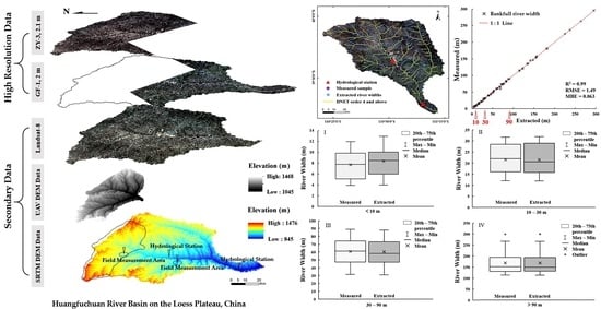
2.1. Study Area

The Huangfuchuan River is located between 110°20′E~111°15′E and 39°12′N~39°59′N. It flows through Zhungeer Banner and Fugu County, Shanxi Province, and joins the Yellow River in Chuankou Village, Fugu County [39]. There are two hydrological stations in the watershed (Figure 1). The main stream of the Huangfuchuan River is composed of the Nalinchuan River (west branch) and the Changchuan River (east branch), with a total length of 137 km, an average slope of 2.7‰, a basin area of 3246 km², and an annual average precipitation of 365 mm. However, the annual precipitation distribution in the basin is extremely uneven, and the precipitation in the flood season (June to September) accounts for 76% of the annual precipitation and 80% of the runoff [40]. The Huangfuchuan River basin has many tributaries and narrow river channels with river widths less than 90 m. We divided rivers narrower than 90 m in the Huangfuchuan River Basin into three categories based on existing studies [5,18] and the resolution of mainstream satellite imagery: narrower than 10 m tiny rivers, 10–30 m thin rivers, and 30–90 m small rivers. The others wider than 90 m are wide rivers. There is no published river surface and width product in this watershed, which is a typical data-deficient area.

2.2. Data Acquisition and Preprocessing

2.2.1. Data Acquisition

Hydrological Data of the Huangfuchuan River Basin

Bankfull discharge and its corresponding bankfull water level, as well as river width, are important parameters reflecting the geometric characteristics of a river channel and the material exchange in the shoal and the floodplain ecological function [35,36]. Therefore, bankfull discharge is used as the criterion to select images in this paper. The measured data of bankfull river width are often obtained by hydrological stations, which are very scarce. To obtain high-precision bankfull river width data in the whole basin through remote sensing imagery, we first need to determine the accurate bankfull discharge and its occurrence date. There are two hydrological stations, Huangfu and Shagedu, in the watershed. The Shagedu station was built in 1990, later than the Huangfu station. Therefore, the runoff data of the two hydrological stations during the flood seasons from 1990 to 2017 were collected and analysed. We verified the consistency of the data by the M-K test method and plotted the measured cross sections of the two stations since the launch of the GF-1 and ZY-3 satellites. A brief introduction to the hydrological data is shown in

Table 1. Summary of the data used in the research.

Type of Data	Data Sources	Data Collection Time	Supplementary Notes
Measured data of runoff and section in Huangfuchuan River Basin	Hydrological data of the Yellow River Basin in the hydrological yearbook of the People’s Republic of China (Volume 4)	Daily average and flood data from 2000 to 2017, and the Measured cross sections data from 2013 to 2017	Shagedu hydrological station in the middle reaches and Huangfu hydrological station at the downstream
GF-1 satellite images	China Center for Resources Satellite Date and Application http://www.cresda.com/CN/, accessed on 5 January 2022	2013, 2016	1A level remote sensing images, 7 scenes
ZY-3 satellite images	China Center for Resources Satellite Date and Application http://www.cresda.com/CN/, accessed on 5 January 2022	2013, 2014	1A level remote sensing images, 3 scenes
Landsat-8 satellite images	Aerospace Information Research Institute, CAS http://ids.ceode.ac.cn/, accessed on 5 January 2022	2013, 2014, 2016	Level 2 remote sensing images preprocessed by the USGS, 6 scenes. Mainly use TIRS bands
FROM-GLC Global Land Use Cover Data	Tsinghua university http://data.ess.tsinghua.edu.cn/, accessed on 12 January 2022	2015, 2017	Terrain Classification and Sampling, 10 m resolution
National land use data	Resource and Environment Science and Data Center https://www.resdc.cn/, accessed on 12 January 2022	2013, 2015, 2017, 2020	Terrain Classification with 30 m resolution
SRTM DEM	Geospatial Data Cloud http://www.gscloud.cn/, accessed on 5 January 2022	2003	SRTM Version 4.1 released in 2015, 90 m resolution
UAV DEM	Produced by our research team	2006	The resolution is 0.88 m

.

According to the in situ measurements of the riverbed elevation conducted in 2013–2015, we calculated the average elevation of the riverbed and obtained the average cross-section form. The result shows that the flood plain only appears at the Shagedu cross section, which can be used to determine the bankfull water level and discharge (Figure 2). According to the definition and estimation method of bankfull discharge [5,36], it is determined that the flood discharge with a water level of approximately 102 m is the bankfull discharge of Shagedu Station, the discharge range is 40–60 m³/s, and the return period is approximately 1.5 years. Since the Huangfuchuan River Basin is a typical data-deficient area, we use the bankfull discharge date of Shagedu station to represent the occurrence date of bankfull discharge in the whole watershed [41].

Multisource Satellite Imagery

The selection of satellite imagery is determined by the bankfull discharge date, but it is difficult to cover the study area under the target date by using one high-resolution image alone, so Chinese GF-1 and ZY-3 high-resolution satellite images were used in combination. The resolution of the GF-1 satellite panchromatic image is 2 m, the multispectral resolution is 8 m, and the revisit period is 1 day. The ZY-3 satellite has a revisit period of 3 days and can provide 2.1 m panchromatic and 5.8 m multispectral imagery products. The overall accuracy index is better than that of French SPOT5 and other similar products [42]. According to the occurrence date of the bankfull discharge, seven scenes GF-1 satellite 1A-level 2 m/8 m images were selected, and the imaging times were 30 July 2013, 23 August 2016, 26 July 2016 and 1 September 2016. Three 2.1 m/5.8 m images of ZY-3 were selected, and the imaging dates were 30 July 2013 and 3 September 2014. To use thermal infrared data to denoise the extraction of the river surface, it is necessary to downscale the low-resolution thermal infrared data. In this research, we adopt the Landsat-8 TIRS bands of 6 scene images during the same period as the GF-1 and ZY-3 images (Table 1). The seamless mosaic images of GF-1 and ZY-3 in the study area without cloud cover are shown in Figure 3a.

Land Use Data

Accurate river surface extraction through machine learning relies on accurate machine learning samples and suitable classification indices. According to the ground feature types in the Huangfuchuan River Basin from 2013 to 2020 based on the existing datasets (Table 1) and Google Earth images, we randomly collected machine learning samples and selected classification indices in the area from which we extracted river surface and downscaled TIRS data. The two types of land use data we refer to showed that the ground feature types in the watershed do not change significantly. We also found that these two datasets were greatly disturbed by mountains and shadows in the source area of the watershed, which resulted in poor river classification.

Measured Data and Samples

In July 2017, we conducted field investigations on eight survey areas in the Huangfuchuan River Basin and marked river and non-river samples. During the investigation, a handheld GPS with a single-point positioning accuracy of 2 m was used to record the location information of 80 samples, and a laser rangefinder with a measurement accuracy of 1 mm was used to measure the bankfull river widths corresponding to the river samples. Because the ground object types in the study area did not change much and there was no large flood flow process after 2016, these 80 measured datapoints can be used as test samples. From the historical Google Earth images, we randomly selected five ground object types, namely, rivers, farmlands, towns, mountains and bare land, in the study area in 2013, 2014, and 2016 as classification samples. The ratio of the five types of samples is 3:2:2:2:1, and all samples cover more than 12 million pixels. We selected all samples following the random principle [43]. The sample distribution is shown in Figure 3b.

DEM Data

In the source area of the watershed, the effect of river surface extraction is strongly influenced by the shadow of the mountain. In addition, the lower-order streams in the source area are generally small in width, which is difficult to extract. To obtain accurate river surface and widths, we used a high-resolution DEM in the source area (Table 1). The data are collected by UAV. The horizontal resolution is 0.88 m and covers 1421 km² in the source area (Figure 4). Other areas in the watershed adopt the SRTM 90 m DEM of version 4.1 released in 2015 (Figure 4). The SRTM DEM is more reliable after manual calibration by NASA than others in the study area, and the elevation accuracy is better than 15 m [44,45,46].

2.2.2. Data Preprocessing

Preprocessing of GF-1, ZY-3 and Landsat-8 Images

GF-1 satellite level 1A imagery is processed by radiometric correction. To ensure the accuracy of waterbody information extraction, it is necessary to perform preprocessing processes, including atmospheric correction, geometric correction, orthorectification, fusion and cropping, on the images [22]. After preprocessing, the GF-1 images are resampled to 2.1 m to match the resolution of ZY-3. The preprocessing process for ZY-3 is automatic calibration, orthorectification, fusion and cropping [47]. We preprocessed images in this study by using ENVI 5.3, and the image stitching accuracy was within 2 pixels. The preprocessing results are shown in Figure 3a.

DEM River Network Extraction

The river network extraction tool (Drainage network extraction tool, DNET) [45] developed by Tsinghua University was used to extract the river network by using SRTM DEM. DNET has been proven to be accurate in extracting the river network and minimizing the problem of parallel river reaches of the river network [45]. When using this algorithm for calculation, the minimum confluence area of the watershed was set to 0.1 km² through repeated experiments, and an 8-order river network was extracted accordingly. The DNET river network is hereinafter referred to as DNET (Figure 4).

3. Research Methods

3.1. RF-ANN River Surface Extraction Method

The extraction method of the river surface consists of three parts (Figure 5):

• The parallelized random forest algorithm improved by a neural network (RF-ANN)
• The denoising method based on the DNET buffer zone
• Morphological postprocessing algorithm

Due to the different spectral characteristics, two types of images should be distinguished in the parallel operation. The compilation environment of RF-ANN is MATLAB, and the running environment is the computer cluster of the State Key Laboratory of Hydroscience and Engineering, Tsinghua University.

3.1.1. RF-ANN Waterbody Extraction Algorithm

Waterbodies (rivers, lakes and others), crops, vegetation and bare land can be effectively distinguished by land surface temperature (LST) in summer, but the spatial resolution of the general land surface temperature products is poor, and it is difficult to be downscaled accurately in a large region [27,28]. LST has not been widely used in ground object classification beyond urban area and river extraction. Moreover, LST cannot be obtained directly from remote sensing images. Therefore, it is necessary to select easily available data that directly respond to LST. We chose thermal infrared data, which can reflect LST and are closely related to the vegetation index [31,32], in this research.

The RF-ANN proposed in this paper used the ANN algorithm based on the four optical bands and vegetation indices of the study area (

Table 2. Commonly used waterbody indices for 4-band high-resolution satellite products.

Spectral Indices	Formula	Reference
Normalized Difference Water Index	NDWI = (B2 − B4)/(B2 + B4)	[1]
Shadow Water Index	SWI = B1 + B2 − B4	[5]
Ratio Vegetation Index	RVI = B4/B3	[10]
Normalized Difference Vegetation Index	NDVI = (B4 − B3)/(B4 + B3)	[11]
New Comprehensive Water Index	NCWI = (7 × B2 − 2 × B1 − 5 × B4)/(7 × B2 + 2 × B1 + 5 × B4)	[12]
Enhanced Shadow Water Index	ESWI = (B1 + B2)/(B4 + B4)	[49]
Green Normalized Difference Vegetation Index	GNDVI = (B4 − B2)/(B4 + B2)	https://www.indexdatabase.de/, accessed on 15 January 2022
Enhanced Vegetation Index	EVI = 2.5 × (B4 − B3)/((B4 + 6.0 × B3 − 7.5 × B1) + 1.0)
Difference Vegetation Index	DVI = B4 − B3
Weighted Difference Vegetation Index	WDVI = B4 − 0.460 × B3
Renormalized Difference Vegetation Index	RDVI = (B4 − B3)/$\sqrt{\left(\mathrm{B}4+\mathrm{B}3\right)}$
Pan Normalized Difference Vegetation Index	PNDVI = (B4 − (B2 + B3 + B1))/(B4 + (B2 + B3 + B1))
Red–Blue Normalized Difference Vegetation Index	RBNDVI = (B4 − (B3 + B1))/(B4 + (B3 + B1))
Blue-Normalized Difference Vegetation Index	BNDVI = (B4 − B1)/(B4 + B1)
Blue-Wide Dynamic Range Vegetation Index	BWDRVI = (0.1 × B4 − B1)/(0.1 × B4 + B1)
Simple Ratio Red/NIR Ratio Vegetation-Index	SRRed_NIR = B3/B4
Adjusted Transformed Soil-Adjusted Vegetation Index	ATSAVI = 1.22 × (B4 − 1.22 × B3 − 0.03)/(1.22 × B4 + B3 − 1.22 × 0.03 + 0.08 × (1.0 + ${1.22}^2$))
Transformed Soil Adjusted Vegetation Index	TSAVI = (0.743 × (B4 − 0.743 × B3 − 0.323))/(B3 + 0.743 × (B4 − 0.323) + 0.413 × (1.0 + ${0.743}^2$))
Visible Atmospherically Resistant Index Green	VARIgreen = (B2 − B3)/(B2 + B3 − B1)
Iron Oxide	IO = B3/B1
Ferric iron, Fe3+	Fe3 = B3/B2
Shape Index	IF = (2.0 × B3 − B2 − B1)/(B2 − B1)
Colouration Index	CI = (B3 − B1)/B3
Redness Index	RI = (B3 − B2)/(B3 + B2)
Color Rendering Index 550	CRI550 = B1−1 − B2−1
Difference 678/500	D678_500 = B4 − B2

B1 is the blue light band, B2 is the green light band, B3 is the red light band, and B4 is the near-infrared band. Same as below.

). The preset downscaled area was within 2.5 km of DNET (90% area of the whole basin), Landsat-8 thermal infrared data (TIR, 30 m) preprocessed by the USGS were used for downscaling to improve the TIR spatial resolution of this area to 2.1 m, and the result was evaluated by cross-validation [48]. Then, waterbodies from the ZY-3 and GF-1 images were extracted by using the RF algorithm in parallel. The parameters of the RF algorithm include indices in Table 2, four optical bands, TIR and texture data (gray-level cooccurrence matrix mean, variance, homogeneity, heterogeneity, correlation, contrast, entropy, energy), for a total of 64 kinds. Synchronized with the RF extraction process is the ANN-based waterbody extraction process using TIR.

After intersecting the ANN extraction result and the RF result, the Kappa coefficient was used to check the accuracy of classification. If the Kappa coefficient is better than the preset accuracy (the preset accuracy can be adjusted), the waterbodies will be output. Otherwise, a circular operation will be performed. To improve the operation efficiency, the parameters of the RF were reselected in accordance with the mean decrease Gini index. Meanwhile, the radius of the downscaling area is reduced by 200 m in each loop along the DNET. The process is looped until the preset accuracy is met or the radius of the operation area is reduced to 1100 m, which is close to the edge of the DNET buffer zone (the range can be adjusted according to the situation of the research area).

3.1.2. Construction and Denoising of the DNET Buffer Zone

The waterbody obtained by the RF-ANN method still contains some noise due to the interference of nearby ground objects such as mountain shadows. To effectively remove noise, we determined the buffer radius of the DNET according to the river orders based on the measured data of the hydrological station and the historical remote sensing images of Google Earth. By taking the intersection between the RF-ANN waterbody result and the DNET buffer zone, the accurate river surface is extracted with less noise.

3.1.3. Morphological Postprocessing Module

The Huangfuchuan River Basin has complex topography and high sediment concentrations. The phenomenon of river blanking is prone to occur inside the river surface, which destroys the connectivity and integrity of the river we extracted. Through experiments, it was found that the use of morphological algorithms can partly solve the problem of holes and river blanking inside the river surface without changing the position and width of the river [22]. Algorithms including equivalent dilation, erosion, bridge and fill are used to morphologically postprocess the river surface products, and finally, the connected river surface with less external noise and basically no holes inside is obtained.

3.2. ARWE Automated River Width Extraction Method

The characteristic river width of a river can reflect the geometric shape of the river channel and can be used as the basic data for the estimation of river material flux transfer. The existing river width extraction methods are often based on manual measurement of the river surface, resulting in low efficiency. Based on the central axis transformation, we established an automated river width extraction (ARWE) method, which has less computation and manual workload. The river widths were extracted based on the RF-ANN method by using the binary river surface data. The method flow is shown in Figure 5.

3.2.1. Automatic Extraction of River Centerline

Automated methods for obtaining river width from remote sensing imagery mostly rely on the river centerline. Existing methods mainly include the RivWidth method (RW) [50], RivWidthCloud method (RWC) [51] and their derivatives [52]. The RW obtains the boundary of the river based on the river surface, makes a large number of vertical lines perpendicular to the boundary and intersects in the river channel, and obtains the centerlines through the intersection of the vertical lines. The RWC obtains the distance gradient of each pixel by performing multiple convolution operations on the binarized river surface data and then manually sets the gradient discrimination threshold to obtain the centerline. Although these methods are automatic, they require manual supervision and a large number of global convolution operations. The skeleton algorithm developed based on the central axis transformation is a typical unsupervised algorithm in morphology. The skeleton algorithm we used is the Voronoi diagram (VD)-based method [53,54,55]. The original code of this algorithm was provided by Zhu, Y. et al. [54]. The VD-based method assumes that the boundary of an input shape Ω is a smooth curve and is sampled by a dense discrete set {P} of pixels. The VD of {P} is computed, and the Voronoi vertices interior to Ω are taken to approximate the central axis. This algorithm ensures that the extracted skeleton adopts the original shape of the objects, and the extraction speed is fast. When the extracted object is in a regular shape, the skeleton is the centerline [56,57,58]. For tiny mountain rivers, the riverbanks do not show strict symmetry. Therefore, the river skeleton obtained is not completely the river centerline because of offsetting in some positions, and needs to be corrected. Based on the above defects of existing methods, we developed the ARWE method, which can automatically correct the river skeleton line to the river centerline. This method does not need to perform convolution operations for all pixels multiple times.

The steps for the ARWE method to extract the river centerline from the river surface are as follows:

The river skeleton is extracted from the river surface by the skeleton algorithm and is defined as the river pseudocenterline after being encoded.

(1)

Calculate the intersection between the orthogonal line of the river pseudocenterline and the river boundary extracted by the morphological edge detection algorithm. The line crossing the intersection points is a pseudo river width cross section.

(2)

Encoding the pseudo river width cross section with the same code as that of the pseudocenterline.

(3)

Calculate and encode the midpoints of each pseudoriver width cross section. The code of each midpoint is recorded as the pseudo river width section. Connecting the midpoints in the order of encoding to obtain the initial corrected river pseudocenterline.

(4)

Cycling steps (1)–(3) until the distance between the midpoints of the same code number obtained from two adjacent calculations is no more than the imagery resolution. Connecting the last calculated midpoints in order of encoding to obtain the ARWE river centerline.

(5)

Assigning the river order attribute of the DNET to each ARWE centerline.

3.2.2. Automatic Extraction of River Width

An automatic extraction of river width generally needs to determine the direction of the river width cross section according to the centerline of the river, and the length of the direction line within the river boundary is the river width. The following takes the automatic extraction of river widths at intervals of 1 km in the whole basin as an example to introduce the steps of determining river widths based on the centerline of the river surface:

(1)

Encoding the source of each order of tributaries as the starting point and the next order’s inflow point as the end.

(2)

The river width sampling points were determined at intervals of 1 km of the centerline (the interval distance can be adjusted). When the length of the tributaries was less than 1 km, the sampling points were constructed near the end. Sampling points are the river width extracted points.

(3)

Constructing reference points upstream and downstream of the extracted points at 10 m intervals along the centerline (the interval can be adjusted according to the image resolution) and then connecting the reference points. The orthometric line of the connecting line was made through the extracted point to determine the direction of the river width section. A schematic diagram of the method is shown in Figure 6a, and the actual effect is shown in Figure 6b.

(4)

Set the length of the direction lines in accordance with the stream order of DNET. Then, the algorithm extracts the intersection points of the direction line and the river surface boundary. The distance between the intersection points is the river width.

3.3. Accuracy Evaluation

We evaluated the extraction accuracy of the watershed from two aspects: one was the evaluation of the river surface extraction; the other was the accuracy of the river widths. The river surface was evaluated by calculating the kappa coefficient [59] of the extraction results, the river extraction accuracy, and the overlay analysis with the DNET, GRWL products, and GSW products in the study area. The extraction ability evaluation of our method was performed by comparing and analysing the extraction results of the more frequently used methods, including the object-oriented method and Otsu from the same data source.

Quantitative evaluation of river width data was completed by linear regression with 80 measured river widths. The average error, R² [60], root mean square error RMSE [61] and mean bias error MBE [62] were chosen as the evaluation indicators.

4. Results and Analysis

4.1. Extraction Results of River surface

4.1.1. RF-ANN Waterbody Extraction Results

The RF-ANN parallel algorithm was used to extract the water bodies of the regions covered by the GF-1 and ZY-3 images. The preset accuracy of the kappa coefficient was 0.6, and the waterbody classification accuracy was 0.75. Based on the 26 explanation vectors proposed in Section 3.1.1, a feedforward neural network (extreme learning machine, ELM) and a BP neural network were designed for downscaling experiments. After six cycles, the downscaled R² of the BP neural network for TIRS-1 within 1.3 km of DNET was 0.82, and the RMSE was 48.4; the downscaled R² of TIRS-2 was 0.84, and the RMSE was 32.6. TIRS data were downscaled well and were used as RF parameters.

RF used downscaled TIRS bands, 26 indices (Table 2), 4 optical bands, and 32 texture indices as classification indicators to classify the watershed to obtain waterbodies. After the trial training of RF, the number of random forest trees was set to 1100, as shown in Figure 7a. The pre-experiment was based on the mean decrease in the Gini index to evaluate the importance of indices. After correlation analysis, 14 indices were determined as the final classification parameters of the watershed, as shown in Figure 7b. The water bodies in the study area were extracted synchronously based on TIRS bands using an extreme learning machine algorithm (ELM). The RF result and the ELM result were intersected, and other types of ground objects were removed to obtain the waterbody.

4.1.2. DEM River Network Constraints and Morphological Postprocessing Results

The radius of the DNET buffer was based on the measurements from Google Earth and hydrological stations. The radius of the river buffer below order 4 rivers was set to 300 m. The river buffer radius of orders 5 and 6 was 600 m, and 1000 m for orders 7 and 8. The river buffer is shown in Figure 8. We take the intersection of the DNET buffer zone and the waterbody in Section 4.1.1 to denoise and initially obtain the river surface.

We use the bridge algorithm, fill algorithm, equivalent dilation and erosion algorithm to fill and connect the interior of the preliminary product of the river without changing the river boundary and obtain an accurate river surface. The waterbody surfaces before denoising are shown in Figure 8a, and the results after postprocessing are shown in Figure 8b.

Figure 9a shows that the RF-ANN method can completely extract the order 4 rivers and most of the order 3 rivers of DNET. The comparisons between RWC river centrelines and ARWE centrelines are shown in Figure 9b.

By comparing the results of the GRWL and GSW datasets, it can be seen that the extraction results of the RF-ANN method show better performance (Figure 10a). In the river source area, where it is difficult to extract rivers, the results based on the same data source of the object-oriented method and the Otsu method were compared. The results show that the river surface obtained by the RF-ANN method has higher integrity with less non-river noise (Figure 10b–d).

4.1.3. Extraction Results of River Centerline and Calculation of River Width

Based on the extracted river surface in the watershed, the ARWE method was used to automatically extract the river width through three steps in Section 3.2.2 and obtain the 1 km bankfull widths in the Huangfuchuan River Basin. There are 153 river widths that match the order 3 DNET, 167 river widths of order 4, 160 river widths of order 5, 114 river widths of order 6, 129 river widths of order 7 and 177 river widths of order 8. The results show that the ARWE river centerline is in better agreement with the rivers in Google Earth than DNET (Figure 9a). We also used the RWC algorithm to extract the river centerline from the same data sources for comparison. The result shows that the ARWE river centerline is more continuous and smooth than the RWC river centerline (Figure 9b). The distribution of all 900 river widths in the watershed is shown in Figure 11.

4.2. Accuracy Evaluation

4.2.1. Verification of the Accuracy of River Surface Extraction

The Kappa coefficient of the RF-ANN river extraction method reaches 0.89, the overall accuracy is 92.1%, and the river extraction accuracy is 94.7%. The total length of the ARWE river centerline is 1023.5 km. The total length of the DNET in the river basin of order 4 and above is 719.8 km, and the length of order 3 and above is 1194.1 km. The abundance of the obtained river is better than that of the order 4 DNET and reaches more than 85% of order 3. In general, this method has a strong extraction ability in mountainous areas with complex terrain and tiny tributaries.

4.2.2. Evaluation of River Width Data Accuracy

The 80 measured river widths were used to verify the ARWE river width accuracy. The results are shown in Figure 12a, and the distribution of the four types of measured river widths is shown in Figure 12b.

The results showed that the average error between the extracted river width and the measured river width in the 80 sets of river width data was 0.97 m, and the image resolution used was 2.1 m, so the extraction error was less than half of one pixel length. R², RMSE, and MBE were 0.99, 1.49, and 0.063, respectively. For the whole watershed, the minimum extracted bankfull river width is 6.1 m (approximately three remote sensing imagery pixels), corresponding with the order 2 DNET, and the maximum is 297.4 m. The analysis of the river width dataset shows that when the sample width of tiny rivers is narrower than 10 m, the average error of extracted river width is 10.9%. For thin rivers with a width of 10–30 m, the average error is 4.9%. The average error of small rivers with widths of 30–90 m is 1.1% and that of wide rivers with widths wider than 90 m is 0.6%. In general, this method is more accurate in the extraction of river width data of different scales in mountainous areas with complex terrain, and the extraction ability is strong.

5. Discussion

In addition to comparing the extraction results of different methods, we also compare the differences between RF-ANN, ARWE and existing methods in terms of algorithms and their principles.

Table 3. Comparisons of existing methods in account of their automation degrees and extraction processes and results.

Algorithms	Time	Method	Automation Degrees	Extraction Processes and Results
RW [50]	2008	Threshold value method	W: Manual judgement, low parallel computation degree	W: Highly dependent on the accurate extraction of river surface, no river surface, low product resolution
OTSU (GRWL, GSW dataset) [10,17,18]	2015, 2018, 2020	Threshold value method	A: Easy principle and operation; W: Manual judgement, low automation degree	A: Small overall workload, small variety of water indices; W: For specific study area, manually measure widths from river surface, high noise interference
RivaMap [52]	2017	Threshold value method	A: Quasi real time water surface extraction; W: Manual judgement of water index during pretreatment of satellite imageries	A: Directly includes river centerlines and river width data, small variety of water indices, W: poor extraction results for mountain rivers, low product resolution
Object-oriented and decision tree [22,23]	2020, 2021	Threshold value method	A: Easy principle and operation; W: Manual judgement, low procedural level.	A: Small variety of water indices; W: Poor river continuity, manually measure widths from river surface, high noise interference
RWC [51]	2020	Threshold value method	A: High computational capacity and efficiency based on GEE; W: Automation degree decreases because of the empirical determination in extracting river centerline and widths.	A: Accurate river surface and width extraction based on convolving river centerline with 9 × 9-pixel kernel in degrees; W: Empirical determination of a pair of 3 × 3-pixel kernels during the river centerline extraction; wider extracted river width due to the not exact perpendicularity of river width to the river centerline, no river surface, low product resolution
Profile features enhance [63]	2021	Threshold value method	A: Easy principle and operation; W: Manual judgement, low procedural level.	A: Small variety of water indices, low-land river, some mountain rivers; W: Manually measure widths from river surface,
RF [5]	2021	Machine learning	A: High computational capacity and efficiency	A: Accurate extraction of river surface, low noise interference W: Manually measure widths from river surface;
RF-ANN	2022	Machine learning	A: High computational capacity and efficiency	A: Accurate extraction of river surface, low noise interference, automatic extraction of river widths, different remote sensing data source; W: Limited downscaling capability of thermal infrared data
ARWE	2022	Machine learning	A: High automation degree, automatic extraction of the accurate river centerline; W: Compiling environment is MATLAB, not able to use in the GEE platform at present	A: Accurate river width due to the exact perpendicularity of river width to the river centerline, different remote sensing data source

A: advantages; W: weakness.

shows the comparisons in detail. The comparison results show that RF-ANN and ARWE have a higher degree of automation, higher computing efficiency, and stronger resistance to noise interference than existing methods. These two methods can be applied to different resolution data sources. Extracting the river surface and width of mountain rivers is an extension of multiple existing methods developed based on Landsat satellites. However, these two methods require parallel processing of a large number of water indices and texture indices and therefore require high performance of computing devices. RF-ANN can only reduce the scale of thermal infrared data to a limited extent, so a more accurate and efficient algorithm that can be applied to a large study area also needs to be developed in the future.

Some tributaries in the watershed were not extracted because of the tiny river surface and high sediment concentration of flowing water, which made the river easily confused with other ground objects. The extracted results of river widths based on ARWE are wider than the measured widths mainly due to the confusion of rivers and other ground objects during extraction, resulting in errors in boundary identification, and the centerlines of some sections of the river being not strictly perpendicular to the real river width section. Even though the minimum bankfull river width is 6.1 m, which corresponds with the order 2 of the DNET, there are still many tiny rivers that were not extracted. In the future, high spatial resolution DEM and radar data will be combined with optical images to explore the automatic extraction of mountainous rivers and gully channels with widths less than 6.1 m under complex terrain to obtain the river and channel width parameters of the whole river network.

6. Conclusions

In this paper, multisource high-resolution satellite images under bankfull discharge dates are used as the main data source. Based on the improved RF algorithm and the central axis transformation algorithm, the RF-ANN river extraction method and the automated river width extraction method, ARWE, are established. The methods successfully extracted the river surface and the river widths of the Huangfuchuan River Basin. The conclusions are as follows:

(1)

We established an improved river surface extraction method, RF-ANN. This automated method consists of three parts. First, we combined the BP neural network and ELM algorithm and successfully improved the RF algorithm. Meanwhile, we realize the parallelization of the improved RF algorithm. Second, based on DEM river network buffer zone constraint denoising, the background noise was almost removed. Finally, the postprocessing on the river surface was based on the morphological algorithm, which solved river blanking and filled holes inside the river surface. This improved method not only has the ability to efficiently extract large-scale river surfaces from multisource satellite images but also makes full use of the texture features of high-resolution images and downscaling thermal infrared data to improve the extraction accuracy by automatically stacking the extraction results of the RF and ANN.

(2)

We developed an unsupervised automated river width extraction method, ARWE. Based on the centerline correction algorithm and the central axis transformation algorithm, ARWE realized the automatic extraction of river width from the river surface. ARWE does not need to go through multiple global convolution operations, and the discrimination threshold does not need to be manually set based on the resolution of the image source, which is more suitable for high-resolution image products and has high extraction efficiency. Theoretically, ARWE can be applied to all optical satellite images.

(3)

We extracted the river surface and bankfull river width of rivers above order 2 in the Huangfuchuan River Basin. The Kappa coefficient of the RF-ANN river surface extraction method reaches 0.89, and the river extraction accuracy is 94.7%. The total length of the river centerline extracted by the ARWE is 1023.5 km, which is more than 85% of the length of the order 3 DEM river network. The average extraction error of river widths, R² and RMSE are 0.97 m, 0.99 and 1.49, respectively. The minimum bankfull river width extracted from the whole basin is 6.1 m (approximately three imagery pixels), which corresponds to order 2 of the DEM river network, and the maximum is 297.4 m.

(4)

In general, the method has a strong ability and high accuracy in extracting river surfaces and widths in mountainous areas. The accurate bankfull river width dataset can be used to (a) enrich the river basic information database; (b) analyse downstream hydraulic geometry and estimate bankfull discharge in river cross sections without hydrological data; (c) provide a more realistic river boundary condition for hydrological models to improve the simulation accuracy; and (d) estimate river carbon emissions.

Due to the limitation of hydrological data under bankfull discharge, this research had some limitations. For example, it is not possible to obtain the basin-wide bankfull data due to the very limited in situ measured hydrological data of the study area; only approximate estimates can be made, so the bankfull river widths we extracted were only approximate widths. We did not analyse the association between parameters of the RF and the subsurface factors of the study area in this research. Therefore, we cannot provide a reference principle for the selection of water indices that can be widely used. In the future, there must be more data sources with high resolution that can be used, and methods with better promotability to improve the extraction of mountain river surfaces and widths.

References

1. Feyisa, G.L.; Meilby, H.; Fensholt, R.; Proud, S.R. Automated Water Extraction Index: A new technique for surface water mapping using Landsat imagery. Remote Sens. Environ. 2014, 140, 23–35. [Google Scholar] [CrossRef]
2. Friedl, M.A.; Sulla-Menashe, D.; Tan, B.; Schneider, A.; Ramankutty, N.; Sibley, A.; Huang, X. MODIS Collection 5 global land cover: Algorithm refinements and characterization of new datasets. Remote Sens. Environ. 2010, 114, 168–182. [Google Scholar] [CrossRef]
3. Li, D.; Wu, B.; Chen, B.; Xue, Y.; Zhang, Y. Review of water body information extraction based on satellite remote sensing. J. Tsinghua Univ. (Sci. Technol.) 2020, 60, 147–161. (In Chinese) [Google Scholar]
4. Frazier, P.S.; Page, K.J. Water body detection and delineation with Landsat TM data. Photogramm. Eng. Remote Sens. 2000, 66, 1461–1467. [Google Scholar]
5. Li, D.; Wang, G.; Qin, C.; Wu, B. River Extraction under Bankfull Discharge Conditions Based on Sentinel-2 Imagery and DEM Data. Remote Sens. 2021, 13, 2650. [Google Scholar] [CrossRef]
6. Mao, H.; Feng, Z.; Gong, Y.; Yu, J. Researches of Soil Normalized Difference Water Index (NDWI) of Yongding River Based on Multispectral Remote Sensing Technology Combined with Genetic Algorithm. Spectrosc. Spect. Anal. 2014, 34, 1649–1655. [Google Scholar]
7. Medina, C.; Gomez-Enri, J.; Alonso, J.J.; Villares, P. Water volume variations in Lake Izabal (Guatemala) from in situ measurements and ENVISAT Radar Altimeter (RA-2) and Advanced Synthetic Aperture Radar (ASAR) data products. J. Hydrol. 2010, 382, 34–48. [Google Scholar] [CrossRef]
8. Sharma, O.; Mioc, D.; Anton, F. Feature Extraction and Simplification from Colour Images Based on Colour Image Segmentation and Skeletonization using the Quad-Edge data structure. In Proceedings of the 15th International Conference in Central Europe on Computer Graphics, Visualization and Computer Vision 2007 in co-operation with EUROGRAPHICS: University of West Bohemia, Plzen, Czech Republic, 29 January–1 February 2007; WSCG 2007, Short Communications. Václav Skala—UNION Agency: Plzen, Czech Republic, 2007; pp. 225–232. [Google Scholar]
9. Wang, H.; Qin, F. Summary of the Research on Water Body Extraction and Application from Remote Sensing Image. Sci. Surv. Mapp. 2018, 43, 23–32. (In Chinese) [Google Scholar] [CrossRef]
10. Li, D.; Wu, B.; Chen, B.; Qin, C.; Wang, Y.; Zhang, Y.; Xue, Y. Open-Surface River Extraction Based on Sentinel-2 MSI Imagery and DEM Data: Case Study of the Upper Yellow River. Remote Sens. 2020, 12, 2737. [Google Scholar] [CrossRef]
11. McFeeters, S.K. The use of the normalized difference water index (NDWI) in the delineation of open water features. Int. J. Remote Sens. 1996, 17, 1425–1432. [Google Scholar] [CrossRef]
12. Zou, C.; Yang, X.; Dong, Z.; Wang, D. A fast water information extraction method based on GF-2 remote sensing image. J. Graph. 2019, 40, 99–104. [Google Scholar]
13. Wang, S.; Baig, M.H.A.; Zhang, L.; Jiang, H.; Ji, Y.; Zhao, H.; Tian, J. A Simple Enhanced Water Index (EWI) for Percent Surface Water Estimation Using Landsat Data. IEEE J. Sel. Top. Appl. Earth Obs. Remote Sens. 2015, 8, 90–97. [Google Scholar] [CrossRef]
14. Acharya, T.; Lee, D.; Yang, I.; Lee, J. Identification of Water Bodies in a Landsat 8 OLI Image Using a J48 Decision Tree. Sensors 2016, 16, 1075. [Google Scholar] [CrossRef] [Green Version]
15. Safavian, S.; Landgrebe, D. A Survey of Decision Tree Classifier Methodology. IEEE Trans. Syst. Man Cybern. 1991, 21, 660–674. [Google Scholar] [CrossRef] [Green Version]
16. Zhang, H.; Wang, D.; Gao, Y.; Gong, W. A study of extraction method of mountain surface water based on OLI data and decision tree method. Eng. Surv. Mapp. 2017, 26, 45–48, 54. (In Chinese) [Google Scholar]
17. Pekel, J.; Cottam, A.; Gorelick, N.; Belward, A.S. High-resolution mapping of global surface water and its long-term changes. Nature 2016, 540, 418–422. [Google Scholar] [CrossRef]
18. Allen, G.H.; Pavelsky, T.M. Global extent of rivers and streams. Science 2018, 361, 585–587. [Google Scholar] [CrossRef] [Green Version]
19. Liu, Z.; Li, X.; Shen, R.; Zhu, F.; Zhang, K.; Wang, T.; Wang, Y. Selection of the best segmentation scale in high-resolution image segmentation. Comput. Eng. Appl. 2014, 50, 144–147. [Google Scholar]
20. Ge, J.; Jiang, Q.; Li, X.; Liu, Y. Comparison and Analysis of Information Extraction Methods of Semiarid Land uti-lization Based on GF1 Image: Taking Jianping as an Example. Glob. Geol. 2017, 36, 1303–1308. (In Chinese) [Google Scholar]
21. Liu, X.; Yu, N. Hierarchical Multi-scale Segmentation of Riverine Wetland Remote Sensing Image. J. Netw. New Media 2016, 5, 51–59. (In Chinese) [Google Scholar]
22. Xue, Y.; Li, D.; Wu, B.; Fu, X. Automatic extraction of small mountain river information and width based on China-made GF-1 satellites remote sense images. Bull. Surv. Mapp. 2020, 3, 12–16. (In Chinese) [Google Scholar]
23. Lu, Z.; Wang, D.; Deng, Z.; Shi, Y.; Ding, Z.; Ning, H.; Zhao, H.; Zhao, J.; Xu, H.; Zhao, X. Application of red edge band in remote sensing extraction of surface water body: A case study based on GF-6 WFV data in arid area. Hydrol. Res. 2021, 52, 1526–1541. [Google Scholar] [CrossRef]
24. Breiman, L. Random forests. Mach. Learn. 2001, 45, 5–32. [Google Scholar] [CrossRef] [Green Version]
25. Acharya, T.D.; Subedi, A.; Lee, D.H. Evaluation of Machine Learning Algorithms for Surface Water Extraction in a Landsat 8 Scene of Nepal. Sensors 2019, 19, 2769. [Google Scholar] [CrossRef] [PubMed] [Green Version]
26. Talukdar, S.; Singha, P.; Mahato, S.; Shahfahad; Pal, S.; Liou, Y.; Rahman, A. Land-Use Land-Cover Classification by Machine Learning Classifiers for Satellite Observations—A Review. Remote Sens. 2020, 12, 1135. [Google Scholar] [CrossRef] [Green Version]
27. Eung, E.M.M.; Tint, T. Ayeyarwady River Regions Detection and Extraction System from Google Earth Imagery. In Proceedings of the 2018 IEEE International Conference on Information Communication and Signal Processing (ICICSP) IEEE, Singapore, 28–30 September 2018; pp. 74–78. [Google Scholar]
28. Pal, M.; Mather, P.M. An assessment of the effectiveness of decision tree methods for land cover classification. Remote Sens. Environ. 2003, 86, 554–565. [Google Scholar] [CrossRef]
29. Wei, H.; Bi, F.; Liu, F.; Liu, W.; Chen, H.; Yu, Y. Water body extraction based on the LBV transformation analysis for China GF-1 multi-spectral images. In Proceedings of the IET International Radar Conference 2015, Hangzhou, China, 14–16 October 2015; pp. 557–561. [Google Scholar]
30. Zhang, Y. A method for continuous extraction of multispectrally classified urban rivers. Photogramm. Eng. Remote Sens. 2000, 66, 991–999. [Google Scholar]
31. Li, L. Experimental Study of the Temperature Variation Characteristic of Some Typical Ground Objects. Master’s Thesis, Northeastern University, Shenyang, China, 2009; p. 82. (In Chinese). [Google Scholar]
32. Wang, A.; Yang, Y.; Pan, X.; Zhang, Y.; Hu, J. Research on land surface temperature downscaling method based on diurnal temperature cycle model deviation coefficient calculation. Natl. Remote Sens. Bull. 2021, 25, 1735–1748. (In Chinese) [Google Scholar]
33. Zhang, X.; Gao, F.; Wang, J.; Ye, Y. Evaluating a spatiotemporal shape-matching model for the generation of synthetic high spatiotemporal resolution time series of multiple satellite data. Int. J. Appl. Earth Obs. 2021, 104, 102545. [Google Scholar] [CrossRef]
34. Raymond, P.A.; Hartmann, J.; Lauerwald, R.; Sobek, S.; McDonald, C.; Hoover, M.; Butman, D.; Striegl, R.; Mayorga, E.; Humborg, C.; et al. Global carbon dioxide emissions from inland waters. Nature 2014, 503, 355–359. [Google Scholar] [CrossRef] [Green Version]
35. Page, K.; Read, A.; Frazier, P.; Mount, N. The effect of altered flow regime on the frequency and duration of bankfull discharge: Murrumbidgee River, Australia. River Res. Appl. 2005, 21, 567–578. [Google Scholar] [CrossRef]
36. Qian, N.; Zhang, R.; Zhou, Z.D. Fluvial Processes; China Science Publishing & Media Ltd.: Beijing, China, 1987; p. 242. [Google Scholar]
37. Wang, G.; Fu, X.; Shi, H.; Li, T. Watershed Sediment Dynamics and Modeling: A Watershed Modeling System for Yellow River. In Handbook of Environmental Engineering; Yang, C.T., Wang, L.K., Eds.; Springer: Cham, Switzerland, 2015; Volume 14, pp. 1–40. [Google Scholar]
38. Yang, D.; Herath, S.; Musiake, K. A hillslope-based hydrological model using catchment area and width functions. Hydrolog. Sci. J. 2002, 47, 49–65. [Google Scholar] [CrossRef]
39. Xu, H.; Taylor, R.G.; Xu, Y. Quantifying uncertainty in the impacts of climate change on river discharge in sub-catchments of the Yangtze and Yellow River Basins, China. Hydrol. Earth Syst. Sci. 2011, 15, 333–344. [Google Scholar] [CrossRef] [Green Version]
40. Wang, B.; Fu, X. Intra-and Inter-annual Variations in the Relationship Between Suspended Sediment Concentra-tion and Discharge of the Huangfuchuan Watershed. J. Basic Sci. Eng. 2020, 28, 642–651. (In Chinese) [Google Scholar]
41. Qin, C.; Wu, B.; Wang, G.; Fu, X.; Zhao, L.; Li, D. Generalized Hydraulic Geometry and Multi-frequency Down-stream Hydraulic Geometry of Mountain Rivers Originated from the Qinghai-Tibet Plateau. J. Hydraul. Eng. 2022, 53, 176–187. (In Chinese) [Google Scholar]
42. Tang, X.; Hu, F. Development Status and Trend of Satellite Mapping. Spacecr. Recovery Remote Sens. 2018, 39, 26–35. (In Chinese) [Google Scholar]
43. Stehman, S.V.; Czaplewski, R.L. Design and analysis for thematic map accuracy assessment: Fundamental principles. Remote Sens. Environ. 1998, 64, 331–344. [Google Scholar] [CrossRef]
44. Mukherjee, S.; Joshi, P.K.; Mukherjee, S.; Ghosh, A.; Garg, R.D.; Mukhopadhyay, A. Evaluation of vertical accuracy of open source Digital Elevation Model (DEM). Int. J. Appl. Earth Obs. 2013, 21, 205–217. [Google Scholar] [CrossRef]
45. Wu, T.; Li, J.; Li, T.; Sivakumar, B.; Zhang, G.; Wang, G. High-efficient extraction of drainage networks from digital elevation models constrained by enhanced flow enforcement from known river maps. Geomorphology 2019, 340, 184–201. [Google Scholar] [CrossRef]
46. Jiang, G.; Xie, Y.; Gao, Z.; Zhou, P. Evaluation on Elevation Accuracy of Commonly Used DEM in Five Typical Areas of China. Res. Soil Water Conserv. 2020, 27, 72–80. (In Chinese) [Google Scholar]
47. Tang, X.; Wang, H.; Zhu, X. Technology and Applications of Surverying and Mapping for ZY-3 Satellites. Acta Geod. Cartogr. Sin. 2017, 46, 1482–1491. (In Chinese) [Google Scholar]
48. Kohavi, R. A Study of Cross-Validation and Bootstrap for Accuracy Estimation and Model Selection. In Proceedings of the International Joint Conference on Artificial Intelligence, Montreal, QC, Canada, 20–25 August 1995. [Google Scholar]
49. Fisher, A.; Flood, N.; Danaher, T. Comparing Landsat water index methods for automated water classification in eastern Australia. Remote Sens. Environ. 2016, 175, 167–182. [Google Scholar] [CrossRef]
50. Pavelsky, T.M.; Smith, L.C. RivWidth: A software tool for the calculation of river widths from remotely sensed imagery. IEEE Geosci. Remote Sens. Lett. 2008, 5, 70–73. [Google Scholar] [CrossRef]
51. Yang, X.; Pavelsky, T.M.; Allen, G.H.; Donchyts, G. RivWidthCloud: An Automated Google Earth Engine Algorithm for River Width Extraction from Remotely Sensed Imagery. IEEE Geosci. Remote Sens. Lett. 2020, 17, 217–221. [Google Scholar] [CrossRef]
52. Isikdogan, F.; Bovik, A.; Passalacqua, P. RivaMap: An automated river analysis and mapping engine. Remote Sens. Environ. 2017, 202, 88–97. [Google Scholar] [CrossRef]
53. Zhong, Y. Computing Medial Axis Transformations of the Geometric Model. J. Comput.-Aided Des. Comput. Graph. 2018, 30, 1394–1412. (In Chinese) [Google Scholar] [CrossRef]
54. Zhu, Y.; Sun, F.; Choi, Y.; Jüttler, B.; Wang, W. Computing a compact spline representation of the medial axis transform of a 2D shape. Graph. Models 2014, 76, 252–262. [Google Scholar] [CrossRef] [Green Version]
55. Chazal, F.; Lieutier, A. The “λ-medial axis”. Graph. Models 2005, 67, 304–331. [Google Scholar] [CrossRef]
56. Blum, H. Biological Shape and Visual Science (Part 1). J. Theor. Biol. 1973, 38, 205–287. [Google Scholar] [CrossRef]
57. Liao, Z.; Wang, Z.; Hu, S. Skeletonize Multi Width Ribbon-like Shapes Based on Difference Images and Frenet Frame. In Proceedings of the 2008 IEEE International Conference on Systems, Man and Cybernetics (SMC), Singapore, 12–15 October 2008; Volume 1–6, p. 839. [Google Scholar]
58. You, X.; Tang, Y. Wavelet-based approach to character skeleton. IEEE Trans. Image Process. 2007, 16, 1220–1231. [Google Scholar] [CrossRef]
59. Landis, J.; Koch, G. Measurement of Observer Agreement for Categorical Data. Biometrics 1977, 33, 159–174. [Google Scholar] [CrossRef] [PubMed] [Green Version]
60. Cameron, A.; Windmeijer, F. An R-squared measure of goodness of fit for some common nonlinear regression models. J. Econom. 1997, 77, 329–342. [Google Scholar] [CrossRef]
61. Singh, J.; Knapp, H.; Arnold, J.; Demissie, M. Hydrological modeling of the iroquois river watershed using HSPF and SWAT. J. Am. Water Resour. Assoc. 2005, 41, 343–360. [Google Scholar] [CrossRef]
62. Ines, A.; Hansen, J. Bias correction of daily GCM rainfall for crop simulation studies. Agric. Forest Meteorol. 2006, 138, 44–53. [Google Scholar] [CrossRef] [Green Version]
63. Zhang, S.; Lu, X.; Lu, Y.; Cheng, L.; Li, M.; Yang, K. Tracking dynamic river networks in the Tibetan Plateau with high-resolution CubeSat imagery. Natl. Remote Sens. Bull. 2021, 25, 2142–2152. [Google Scholar]
Figure 1. Schematic diagram of the Huangfuchuan River Basin. Photo (A) was taken in the upper reaches of the river basin. Photo (B) was taken in the middle reaches of the river basin.
Remotesensing 14 02370 g001
Figure 2. Average cross-section morphology of the Shagedu hydrological station.
Remotesensing 14 02370 g002
Figure 3. Data sources and samples in the study area. (a) The multisource remote sensing data of the Huangfuchuan River Basin used in this research. (b) The distribution of machine learning samples and validation samples in the Huangfuchuan River Basin. (c) Land use types in the Huangfuchuan River Basin. Region I shows the poor results of waterbody extraction in the source area.
Remotesensing 14 02370 g003
Figure 4. UAV DEM, SRTM DEM and river network in the Huangfuchuan River Basin.
Remotesensing 14 02370 g004
Figure 5. Technical route of river surface and river width extraction.
Remotesensing 14 02370 g005
Figure 6. Key steps and illustration of the river width cross sections. (a) Method for determining the direction of river width and calculating the river width at the river width extracted points. (b) Schematic diagram of the river width cross section at the extracted points.
Remotesensing 14 02370 g006
Figure 7. Result of the RF algorithm pre-experiment. (a) RF parameter optimization. (b) The final selection of classification index and importance ranking.
Remotesensing 14 02370 g007
Figure 8. Effect of the river surface denoise. (a) Schematic representation of preliminary waterbodies extraction results. River blanking and the noise were shown. (b) River network buffer zone constraints and postprocessing results.
Remotesensing 14 02370 g008
Figure 9. The extraction result of the river surface. (a) Comparisons between all the extracted rivers and river networks above order 2 that were generated from a 90-m resolution DEM. (b) Comparisons between RWC river centerline and ARWE river centerline. The cut-off and omit region of RWC river centerline was shown.
Remotesensing 14 02370 g009
Figure 10. Comparison with different river surface datasets and extraction methods. (a) Waterbodies extraction results of existing products in the Huangfuchuan River Basin. Part I shows the unconnected rivers. (b) River surface extraction result of RF-ANN in the river source area. (c) River surface extraction result of the object-oriented method based on multiscale segmentation in the source area. (d) River surface extraction result of OTSU in the source area.
Remotesensing 14 02370 g010aRemotesensing 14 02370 g010b
Figure 11. The river widths dataset extracted by ARWE method. (a) ARWE river widths data distribution in the Huangfuchuan River Basin. (b) Number of river reaches with and without bankfull width information of order 3 DNET.
Remotesensing 14 02370 g011
Figure 12. Accuracy evaluation of the river widths. (a) Comparison between the extracted river widths and measured data. (b) Distribution diagram of measured river widths. (c) The difference between measured and extracted widths of tiny, thin, small and wide rivers was shown separately in the form of box plots.
Remotesensing 14 02370 g012