Article

Challenges in Diurnal Humidity Analysis from Cellular Microwave Links (CML) over Germany

1
Department of Geophysics, Porter School of the Environment and Earth Sciences, Raymond and Beverly Sackler Faculty of Exact Sciences, Tel Aviv University, Tel Aviv 6997801, Israel
2
The Fredy and Nadine Herrmann Institute of Earth Sciences, The Hebrew University of Jerusalem, Jerusalem 9190401, Israel
3
Department of Environmental Physics, Environmental Sciences Division, Israel Institute for Biological Research, Ness-Ziona 7410001, Israel
4
Institute of Meteorology and Climate Research, Karlsruhe Institute of Technology, Campus Alpin, 82467 Garmisch-Partenkirchen, Germany
*
Author to whom correspondence should be addressed.
Remote Sens. 2022, 14(10), 2353; https://doi.org/10.3390/rs14102353
Submission received: 22 March 2022 / Revised: 26 April 2022 / Accepted: 7 May 2022 / Published: 12 May 2022

Abstract

:
Near-surface humidity is a crucial variable in many atmospheric processes, mostly related to the development of clouds and rain. The humidity at the height of a few tens of meters above ground level is highly influenced by surface characteristics. Measuring the near-surface humidity at high resolution, where most of the humidity’s sinks and sources are found, is a challenging task using classical tools. A novel approach for measuring the humidity is based on commercial microwave links (CML), which provide a large part of the cellular networks backhaul. This study focuses on employing humidity measurements with high spatio–temporal resolution in Germany. One major goal is to assess the errors and the environmental influence by comparing the CML-derived humidity to in-situ humidity measurements at weather stations and reanalysis (COSMO-Rea6) products. The method of retrieving humidity from the CML has been improved as compared to previous studies due to the use of new data at high temporal resolution. The results show a similar correlation on average and generally good agreement between both the CML retrievals and the reanalysis, and 32 weather stations near Siegen, West Germany (CML—0.84, Rea6—0.85). Higher correlations are observed for CML-derived humidity during the daytime (0.85), especially between 9–17 LT (0.87) and a maximum at 12 LT (0.90). During the night, the correlations are lower on average (0.81), with a minimum at 3 LT (0.74). These results are discussed with attention to the diurnal boundary layer (BL) height variation which has a strong effect on the BL humidity temporal profile. Further metrics including root mean square errors, mean values and standard deviations, were also calculated.

Graphical Abstract

1. Introduction

The near-surface humidity is a crucial variable in many atmospheric processes, mostly in those related to development of clouds and rain. Measuring humidity at high spatial-temporal resolution is important for meteorological and agricultural applications. The humidity behavior and its spatial patterns are dictated by several elements in a variety of scales; thus, it is not enough to rely on the existing coarse observation systems. The large-scale elements that control the humidity are weather patterns at the synoptic scale which can transfer humidity over long distances by advection and further be modified by factors like complex topography, planetary boundary layer (PBL) dynamics, and land cover (LC). The humidity at the height of a few tens of meters above the surface is highly influenced by surface characteristics which can act as a humidity sink or source. Measuring the near-surface humidity at high resolution, where most of the humidity’s sinks and sources are found, is challenging with classical tools. This near-surface humidity field is often the most important variable for convection predictions [1,2]. Currently, humidity fields are predominantly obtained by surface stations, radiosonde, and from satellite remote-sensed data. Surface stations provide point observations, and therefore may suffer from low spatial representation. Furthermore, humidity is a field with unusually high mesoscale variability, as demonstrated by structure functions [3]. In addition, there is a limited ability to deploy humidity gauges in heterogeneous terrain or in areas with complex topography. Satellites do allow for a large area to be covered in high spatial and temporal resolution, but are frequently not accurate enough in the atmospheric boundary layer and depend on surface emissivity and cloud cover [4]. Radiosondes, which are typically launched only 2–4 times a day, also provide very limited information due to generally much low spatial and temporal resolution. Additionally, radiosondes are quite costly for implementation, deployment, and maintenance, and they gain height quickly, thus missing information at the lower boundary layer. Because of different surface perturbations, a point measurement close to the surface (for example, 2 m above ground, as required for a standard meteorological surface station) is often not satisfactory for model initialization through data assimilation. An ideal requirement for meteorological modeling purposes would be an area-averaged measurement of near-surface humidity over a “box” with the scale of the model’s grid and at an altitude of a few tens of meters, which often better fits the lowest model layer [5]. Current conventional measuring tools cannot effectively provide such data.
The method for humidity measurements presented here, however, provides a unique way of obtaining precisely the required type of near-surface information and is based on data collected by wireless communication networks through the so-called commercial microwave links (CML). This data was first exploited to derive rainfall information [6,7,8,9,10]. The technique introduced here to measure atmospheric near-surface humidity using CML data was originally proposed by David et al. [11]. This work proved the concept of retrieving near-surface humidity from CMLs at frequencies around 22.23 GHz. This was further developed by Alpert and Rubin [12], where maps of near-surface humidity over Israel from high density CMLs were produced for a single time of the day (0200 LT). These maps were shown to have lower root mean square error (RMSE) as compared to conventional operational surface humidity data. Recent studies have shown the potential and the ability of harnessing the CML at high frequencies (E-bands) which are more sensitive to the changes of humidity but are often shorter, and thus are not always compatible for humidity detection [13,14]. In addition, research on the ability to measure the humidity based on low CML frequencies was also performed [15]. This study emphasizes the potential of the cellular infrastructure to provide large amounts of data which can potentially be used as humidity observations at a high temporal and spatial resolution.
Meteorological weather forecasting heavily relies on atmospheric models, the accuracy of which is largely determined by the quality of its initial conditions. The large number of observations from the cellular network have the potential to increase the amount of data assimilated into weather forecast models, and, in turn, improve initial conditions (analyses) and forecasts. Humidity, in particular, has a crucial role in model initialization [16]. The near-surface humidity is often responsible for convection initiation, especially over continents, which may occur at smaller scales relative to the coarser fields described by current observational tools (mostly based on weather stations). The lack of moisture constraints is exacerbated by heterogeneity in land–surface conditions and our inability to represent boundary layer dynamics with current numerical weather prediction (NWP) model resolution for weather forecasting, such as WRF and COSMO (e.g., [17,18]).
The CMLs are deployed at high-spatial density and often available at high temporal resolution. Consequently, they can provide a more complete picture of the near-surface humidity field and improve the resolution of the humidity information for assimilation in the NWP models. A high-resolution description of the near-surface humidity could better capture the smaller scale spatial variations often caused by water vapor condensation into drops and by small-scale atmospheric flow, for example, advection of humidity after rain at local scales.
While the great value of the humidity data in rainfall studies is well-known, especially in hydrology, ecology, and climate, these data have only been exploited by NWP in recent years. This was made possible as a result of the increasing availability of remotely sensed humidity observations [19,20], together with advances in modeling and data assimilation [21,22]. These observational constraints are especially relevant at convective scales [23], where higher model resolution demands denser observations at a suitable spatio–temporal resolution for representing mesoscale phenomena.
In this study, we will explore the use of humidity measurements at high spatio–temporal resolution, based on CML data at a high signal resolution (low QE, meaning quantization error) in Germany. One major goal of this work is to assess the skill and the environmental influences on the CML observation by comparing the CML humidity observations (CML-HO) to weather station humidity observations (WS-HO) and reanalysis products at ~6 km (0.055°) grid-size resolution over Germany (COSMO-REA6, hereafter Rea6, by Germany’s National Meteorological Service, Deutscher Wetterdienst, (DWD, https://opendata.dwd.de/climate_environment/REA, accessed on 24 March 2021). All the data sources refer to absolute humidity measured in g/m3. The CML-HO fields were produced at high resolutions and the mean diurnal CML-HO patterns interpolated at the weather stations’ locations were calculated and compared at different times of the day. The high temporal resolution allows, for the first time, an evaluation of the method used in previous research for retrieving CML-HO [11,12] during different diurnal periods. Here, we tested the calibration method, based on additional statistical information and assumptions about the state of the atmosphere, in different configurations and for different CML characteristics.
The paper is organized as follows: In Section 2, the methodology is described with an emphasis on the calibration methods to retrieve the CML-HO data. Section 3 presents the comparisons between CML-HO and reanalysis (Rea6) to WS-HO and analyzes the main outcomes. Moreover, Section 3 focuses on the cases where disagreements between CML-HO and WS-HO were observed and discusses possible causes for them. The main conclusions are summarized in Section 4.

2. Methodology

2.1. Study Region and Data

This study focuses on the region between the latitudes 50–51.3°N and the longitudes 7–9°E (the size of ~145 km × 220 km) (see Figure 1).
The total number of CMLs used within the study region is 517, with frequencies in the range of 13.1–33.2 GHz. CML lengths were chosen to be between 5 and 10 km. This allows us to more easily detect the humidity changes and reduce the error due to the resolution limitation of the CML data in terms of QE (further details in Section 2.2). The QE of the received signal level (RSL) data was 0.3 dB, while the QE of the transmit signal level (TSL) was of 1 dB. The CML data recordings were taken as instantaneous values every minute. The comparison to WS-HO and Rea6 was done for a lower temporal resolution of one hour. Therefore, the total attenuation, γ, is calculated from Equation (1):
γ = TSL − RSL
The total attenuation, γ, was averaged for the last 10 min of each hour to represent the full hour’s records and in order to reduce instrumental or environmental errors typical in some of the instantaneous values [24]. The CML-HO spatial interpolated field obtained following a Cressman interpolation method (see Section 2.5) was compared to WS-HO values at 32 weather stations inside the study region. The stations’ names and elevations above mean sea level (AMSL) are listed in Table 1. The locations of the CMLs and the weather stations are presented in Figure 1. The WS-HO data were also compared to Rea6 humidity at the level of approximately 30 m above ground level (AGL). The Rea6 has a high resolution compared to the commonly used reanalysis ERA-Interim [25] and ERA5 [26], and therefore we expected it to better represent near-surface and PBL processes, in particular, humidity, a major difference from the Alpert and Rubin study [12]. The period examined in this study is June 2018, which is characterized by relatively large inter-daily humidity variations and heterogenous weather conditions, including dry and wet periods.

2.2. Humidity Retrievals from Commercial Microwave Links

The attenuation of a microwave signal due to water molecules is most significant at the resonance line of 22.235 GHz [11]. The specific attenuation γ (dB/km) due to dry air and water vapor (WV) can be evaluated using Equation (2) (Rec ITU-R P.676-12 (2019) [27,28], assuming no rainfall, fog, clouds, and strong winds are present, as follows:
γ = γv + γd + Ñoise
where γv and γd are the specific attenuation due to WV and dry air (i.e., oxygen, pressure-induced nitrogen, and non-resonant Debye attenuation), respectively. Ñoise are all other signal perturbations as a result of factors other than WV. Apart from the strong diurnal patterns and erratic noisiness that we will discuss later, the terms γd and Ñoise are usually one order of magnitude smaller than γv for microwave signals with frequencies around the resonance line. As such, the measured RSL can be related to WV by:
γ v = 0.182 f   N ( f ) ,   where   N ( f ) = i ( O x y g e n ) S i F i + N D ( f ) + i ( W a t e r   V a p o u r ) S i F i  
N″(f) is the imaginary part (absorption) of the complex refractivity, which is a function of the link’s frequency f (GHz), pressure p (hPa), temperature T (°C), and WV density ρ (g/m3), which is the quantity to be retrieved from the measured signal γ. N″(f) can be expressed as a function of S i , the strength of the i-th WV line, and F i is the WV line shape factor. N D ( f )   is the dry continuum due to pressure-induced nitrogen absorption and the Debye spectrum. Further information on spectroscopic data for WV attenuation can be found in Rec ITU-R P.676-12 (2019).
By knowing the specific attenuation γ which is approximated to be mostly γv, the humidity (in WV density units) can be obtained by inverting Equation (2). Note that we need to know T and p along the path of link sites. Errors in T and p were found to lead to smaller errors in humidity calculation, and then in those resulting from the minimal interval of the RSL measurements (QE) ([11,12], examples can be seen in [29]). The QE, along with the CML length, mainly determines the error range. The length-related error arises from the fact that we calculate the average value of the true humidity along the link’s path by dividing the attenuation due to WV by the link’s length to obtain the normalized attenuation in dB/km, thus assuming a homogenous WV distribution along the link. There is a tradeoff: the longer the link, the better the signal to noise ratio; but we might then miss spatial variations along the link’s path with longer CMLs. On the other hand, for shorter CMLs it may be difficult to measure the true humidity temporal variations (if errors are too large, the low signal to noise ratio makes it difficult to filter out physical variability of the humidity from noise fluctuations). Thus, we are limiting the length of the used links to be between 5 and 10 km. In previous studies, shorter links were included and showed good correlations with weather stations [11,12,30]. In this study, we had enough observations to choose only the longer links, which slightly improves the performances and reduces the error due to temperature and pressure accuracy along the CML (Equation (3)).
The cellular data include information on the transmit signal level (TSL) as well, so we can calculate the total attenuation, γ, changes in time (Equation (1) above). In order to calculate γd and retrieve γv from Equation (2), we use auxiliary information from the weather stations as described in Section 2.3.

2.3. Calibration

Since every CML has a different γ range and characteristics (length and frequency), the γd of each CML at given air conditions T and p is different, too.
Following Equation (1), γd may be expressed as in Equation (4), i.e., by defining RSLo, the contribution to the total RSL that results from dry air.
γd = TSL − RSLo
Combining Equations (1), (2) and (4), RSLo can be expressed as in Equation (5), (where averaging over a period was performed, and therefore noise can be neglected).
RSLo = RSL − γv
Therefore, we are left with the need to calculate RSLo for each link. In an attempt to do so, we note that RSLo is not expected to change to a large extent from day to day, in particular, within the same season and time of the day. We take advantage of WV measurements at stations to estimate RSLo for nearby links. Assuming that the WV at the stations, WS-HO, and at nearby CMLs and CML-HO, which are approximately the same, we use past RSL values of the link (RSLp) and past WV measurements at stations, WS-HOp, to retrieve RSLo. Using the past WS-HOp as a proxy of CLM-HOp along the CML, we estimate the past values of γv at the link, γvp, using Equation (3), and retrieve RSLo from Equation (5) as follows (Equation (6)):
RSLo = RSLp − γvp
Equation (6) is calculated over a period of time to cancel noise, e.g., 2 weeks. The median values of RSLo from the 2 week period of calculations, RSLom for each link, are then used to calculate future values of γv. By subtracting Equations (1) and (4), γv is calculated as follows:
γv = RSL − RSLom
The method described above was used in previous works [11,30]. There, the WS-HOp and the γvp were calculated based on the closest weather stations to the link in order to estimate the RSLo (Equation (6)). However, in areas of complex terrain, the nearest station to a given CML can exhibit different humidity patterns than the CML if the height differences between them are significant. In Alpert and Rubin, 2018, and in this work, we use a different method, as described below.
First, the median of the WS-HO, WS-HOm, from each weather station over the study area was calculated for a two week period, for each hour of the day separately. Then, the calibration (finding the RSLo of each individual CML) was done based on the assumption that, on average, the absolute humidity along the CML decreases with elevation AMSL. Figure S1 shows the variation of WS-HO with elevation AMSL over the Siegen region in Germany.
Linear equation relationships between the WS-HOm at each station and its height AMSL, h, over the study area were derived. These equations represent the absolute humidity dependence on height AMSL. The calculations were performed for the period between 18 May and 31 May 2018. Two approaches were adopted to calculate the linear equations. In one of them, the linear equations were calculated for each hour of the day (named cali1), while in the other, a single linear equation was calculated for all hours of the day together (cali2). Equation (8) is the linear equation for all hours of the day together, i.e., the cali2 approach. Once these linear equations were derived, values of CML-HOp needed to derive RSLo (Equations (4)–(7)) could be calculated at the mean heights AMSL, h, of each CML, using either the cali1 or cali2 approach.
W S H O m   ( h ) = 0.0027 h + 12.06
Equation (8) describes the linear dependence of WS-HOm on h, the elevation AMSL. The fitted equations change with seasons and the climate zone; therefore, the equation was produced for the two week period prior to our study.

2.4. Optimization of RSLom Calculation

In order to find the best approach for calculating RSLom, we used several time intervals (e.g., 1, 6, and 24 h) as described in Section 2.3, following the cali2 method. Once the various values of RSLom were calculated, we used them to estimate future values of CML-HO and compared those to nearby WS-HO. In order to do so, we interpolated single links values of CML-HO into a regular grid of 1 km × 1 km resolution and used the interpolated CML-HO at the grid points closest to the weather stations. The interpolation method employed here is based on the distance-weighted method by Cressman [31] (see Section 2.5). Correlation and root mean squared errors (RMSE) between interpolated CML-HO and WS-HO were calculated for a period of one month using all weather stations. The 24 h interval showed the best correlation values. RMSE errors were not very sensitive to time intervals, but different periods of the day were sensitive to the choice of cali1 or cali2 under the use of a 24 h interval. For example, late night and early morning (until 6 LT) achieved better results with the cali2 approach, while morning hours after 6 LT cali1 showed lower RMSE, on average (see Figure 2 and Table 2).

2.5. Interpolation

As stated in Section 2.4, the CML-HO at single CMLs were interpolated to a regular grid at 1 km × 1 km resolution. These were, in turn, compared to WS-HO using the values at the closest grid point to the station. The interpolation method employed here is based on the distance-weighted method for interpolation by Cressman [32]. In the interpolation, we considered three CML-HO observation points along the CML, two at the edges, and one in the middle. This method was found to be the most accurate for CML-HO fields [12,30]. The radius of interpolation for the inverse distance weighting was chosen to be 40 km since other smaller radii that were tested showed lower correlation and higher RMSE between CML-HO and WS-HO for most of the weather stations (radii larger than 40 km were examined, too, and no significant differences were observed). This kind of comparison was done before in Israel as well, where the same results were obtained [30]. At a few stations only, radii smaller than 40 km produced better results. These stations appeared to be located over a region of complex topography. David et al. [30] demonstrated that if we consider all CMLs over a large region around the weather station’s grid point in the interpolation (inside the 40 km radius), we will better estimate the true absolute humidity, i.e., a lower error and better correlation with the nearest station.

2.6. Analysis Methods

To evaluate the skill of the CML-HO against the reference data set, the WS-HO, we used four skill scores metrics: the correlation, the RMSE, the mean, and the standard deviation (STD) [32] (see full results in Table 2). In addition, a similar evaluation was done for the Rea6 humidity at ~30 m AGL using the closest grid point to the weather station location. The Rea6 was considered as an additional reference representing a spatial mean of the humidity field at a 6 km × 6 km grid size. Rea6 is obtained by the data assimilation of observations into a numerical weather prediction model; therefore, it is the result of an optimal combination of dynamical model calculations and observations. The WS-HO here represents local phenomena as compared to the interpolated values from the Rea6 and the CML-HO fields.
The correlation was calculated based on Pearson’s linear correlation, which is a measure of the linear correlation between two sets of data. It is the ratio between the covariance of two variables and the product of their standard deviation. The Pearson’s linear correlation coefficient is calculated based on Equation (9):
C o r r ( a , b ) = i = 1 n ( X a , i X a ¯ ) ( Y b , i Y b ¯ ) { i = 1 n ( X a , i X a ¯ ) 2 j = 1 n ( Y b , i Y b ¯ ) 2 }  
where n is the length of each data set. Values of the correlation coefficient can range from −1 to +1. A value of −1 indicates a perfect negative correlation, while a value of +1 indicates a perfect positive correlation. A value of 0 indicates no correlation between the columns.
The root mean square error (RMSE) is the square root of the average of the squared errors. In this case, the errors are the differences (residuals) between the WS-HO and CML-HO. the RMSE is calculated based on Equation (10):
R M S E = t = 1 T ( x 1 , t x 2 , t ) 2 T
where x 1 , t   is the WS-HO, x 2 , t   is the CML-HO or the Rea6 humidity values at a specific time, and T is the number of observations. The RMSE represents the deviations between the CML-HO and Rea6 from the observed humidity at the stations (WS-HO).
Differences in mean values between the different data sources represent systematic differences (bias) between them. The STD is an indication of the range of humidity fluctuations in the three sources of data. Disagreement in the means and STDs between the different sources may arise due to various micro and meso scale processes that differently affect the CML-HO, WS-HO, and Rea6 values.

3. Results

This section summarizes the main outcomes from the data analysis. The availability of RSL and TSL at a high temporal resolution allows the investigation of several behaviors during the diurnal cycle. Moreover, it enables us to highlight questions about the diurnal patterns of the CML-HO and the diurnal variations of several measures, such as correlation and RMSE. These, in turn, can reveal some of the potential environmental impacts on the CML attenuation that are not necessarily related to the true absolute humidity at the CML location.
We define daylight hours as those between 9–17 LT and nighttime hours as those between 18–8 LT. All of the CML-HO values were calculated for the 24h interval calibration method and an effective radius for interpolation of 40 km.
The next sections summarize the results in three main sub-titles: the findings from the statistical evaluation, those about the mean diurnal cycle, and those about the inter-daily variability.

3.1. Statistical Evaluation

Figure 2 and Table 2 summarize the results. The main conclusions from the comparisons of the CML-HO and Rae6 with WS-HO are as follows:
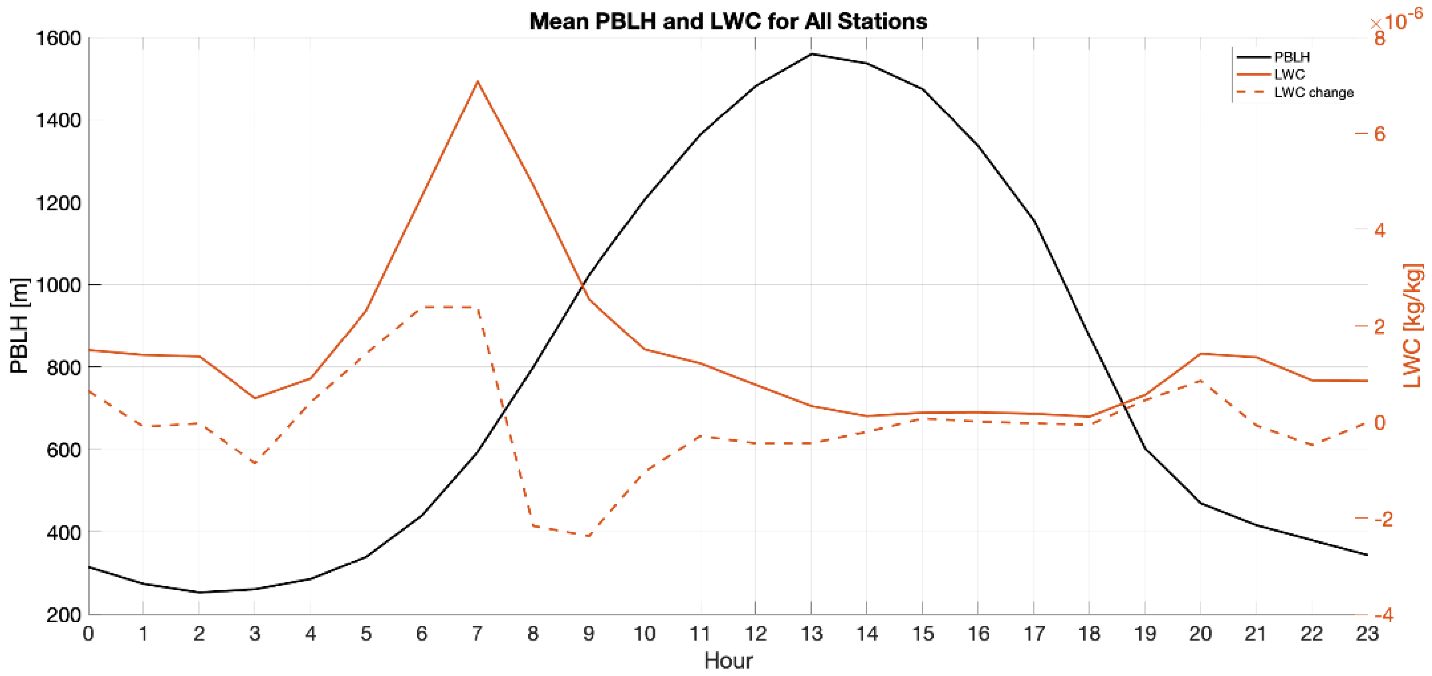
  • All sources (WS-HO, CML-HO, and Rea6) show maximum mean values of humidity during nighttime hours and minimum mean values during daylight hours, as expected from the minimum and maximum values of the PBL heights (PBLH), respectively (see Figure 3). The STD values for all sources are of the order of 20% of the mean values.
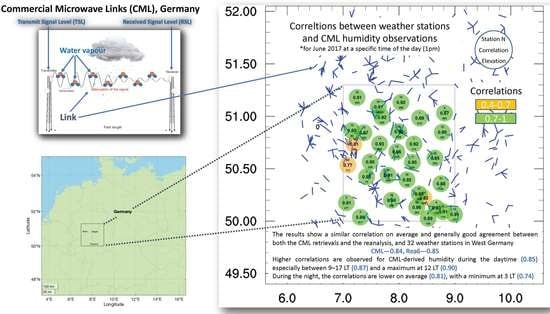
  • Focusing on correlations, the WS-HO show high correlations with both CML-HO and Rea6, with average values of about 0.84 and 0.85, respectively. During most hours, the correlation was higher between the Rea6 and the WS-HO (17 out of 24 h) than between CML-HO and WS-HO (7 out of 24 h). Notice, however, that during daylight hours, there is a slight advantage for CML-HO (0.87 vs. 0.84). At night, the correlations between Rea6 and the WS-HO are higher than those between CML-HO and WS-HO (0.86 vs. 0.82, respectively).
  • The RMSE is smaller in the case of Rea6 than CML-HO for most of the hours (18 h, with averages of 1.49 vs. 1.58, respectively), except during daylight.
  • Mean and STD: The CML-HO mean and the STD values are closer to the WS-HO values, on average, than those of Rea6 (10.12 vs. 10.74 vs. 10.04 and 2.26 vs. 2.21 vs. 2.29, respectively), but during the day light hours, the Rea6 mean and the STD are closer to those of WS-HO, which is just the opposite to the correlation and RMSE behavior.
It should be noted that due to the lack of in situ observations at the level of ~30 m AGL, comparable to the CML altitudes, the validation can be performed only by comparing the CML-HO and Rea6 humidity to WS-HO (at ~2 m). Comparing different levels of the atmosphere can generate errors under stable atmospheric conditions. The true absolute humidity can be different between low levels of the atmosphere for low inversion conditions at night, for example. Still, in terms of correlations with WS-HO, we can see that the behavior is captured quite well for both sources (CML-HO and Rea6).

3.2. Mean Diurnal Cycle

Figure 2 shows the mean diurnal cycles over the studied period. Mean (panel a) and STD (panel b) of CML-HO, WS-HO, and Rea6, and the correlation (panel c) and RMSE (panel d) between WS-HO and both sources, CML-HO and Rea6, averaged over all the stations’ locations and all the metrics averaged over all the stations’ locations.
Looking at the mean values (Figure 2a), we clearly see that WS-HO and Rea6 follow a quite similar diurnal pattern, with two main differences: WS-HO shows local maxima at 5 LT and 19 LT is not observed in Rea6, and Rea6 is negatively biased with respect to WHSO at all times, with the largest biases at the times when the WS-HO local maxima occur. This Rea6-WS-HO bias is expected due to the height differences between WS-HO measurements (2 m AGL) and Rea6 (30 m AGL), as humidity is expected to decrease with height. The CML-HO cali2 mean values closely follow the pattern and values of Rea6 between 10–23 LT. This has good agreement between the CML-HO and Rea6 and is likely to be observed as both CML-HO and Rea6 are at the same height (30 m AGL) and represent a spatial mean value (1 km and 6 km grid for the CML-HO and Rea6, respectively) as opposed to the local representativeness of WS-HO point observations. However, at earlier times, we notice disagreement between the three sources. The cali1 pattern is similar during daylight; however, after 18 LT, it has higher values in comparison to Rea6 and cali2. Between midnight and 10 LT, the CML-HO behavior, for both methods (cali1/cali2), is characterized by a non-monotonic decrease observed in neither WS-HO nor Rea6. This behavior reveals the complexity of CML-HO retrievals at nighttime hours, which will be further discussed.
Another feature that we notice in the mean CML-HO values is its steep increase between 17–19 LT in comparison to the WS-HO and Rea6 values for the cali1 case (Figure 2a). This is still evident in some stations when applying the second method for calibration (cali2, not shown here). Considering that these are early morning and evening hours, the excess mean CML-HO may result from increased attenuation due to other factors, rather than from WV, such as condensation of water in the air due to the nocturnal temperature drops, advection of fog, or condensation of water on the antenna [33,34,35,36]. The LWC (liquid water content) average diurnal pattern for all the stations, shown in Figure 4, implies condensation of WV during the early morning hours when the PBLH and the temperatures are, on average, relatively low.
Focusing on STD values (Figure 2b), the STD reaches its highest values at 16 LT for the WS-HO and the Rea6, and at 18 LT for the CML-HO. In general, all sources have a high STD during the late afternoon hours between 16 LT and 18 LT, while their diurnal behavior is quite different. The WS-HO, which represents the lowest level AGL among the three sources, has low STD during the nighttime hours, with the minimum observed at 3 LT and then a gradual increase until it reaches its maximum value at 16 LT. The Rea6 shows a similar behavior to WS-HO, with relatively low values of STD at night. However, the minimum Rea6 STD is observed at 10 LT. The Rea6 is also characterized by higher STD values at night when compared to the WS-HO STD. The differences between WS-HO and Rea6 STD can arise from the different level that each of them represents. When looking at the CML-HO STD behavior, the minimum values are observed at 9 LT, close to the Rea6 minimum STD time. However, the CML-HO STD general pattern is different from both WS-HO and Rea6. The CML-HO STD is higher compared to the other sources at night and decreases at 5 LT to be lower than both. The CML-HO STD remains low during the early part of the day until 14 LT, when it increases again. We notice a large difference between the CML-HO and WS-HO STDs after midnight, which implies that night conditions might affect the CML retrievals differently than day conditions, and thus lead to larger day to day variability.
To better understand the differences between the mean CML-HO and WS-HO diurnal pattern, we analyze the diurnal cycle of both (CML-HO and WS-HO) at different locations and search for similarities between the observed patterns. For most of the stations in the research domain, the diurnal cycle of the WS-HO shows a similar diurnal pattern at night and in the evening for all stations. The average diurnal pattern is characterized by low values of humidity during daylight and high values during nighttime (Figure 2a). On average, the WS-HO follows the PBLH during the day (Figure 4), which is low at night and closer to the surface, and higher during daytime. The height of the PBL is defined as the level where the inversion base is located; thus, it is the boundary between two layers with quite different characteristics, such as absolute humidity and temperature ([37], Figure 1.9; [38], for similar conditions in Germany; [39], for Israel). During daytime, the layer below the inversion is well-mixed and the vertical profiles of humidity and temperature are nearly homogeneous above the so-called surface layer. At night, the inversion altitude drops and the layer below it gets shallower. Assuming that there are no significant changes in the PBL vertically integrated WV during the day, i.e., no significant changes due to weather systems and advection (large changes are often caused by advection, e.g., [37], Figure 1.7), the absolute humidity is expected to increase at night due to the reduction in the total volume of the lower moist layer that became shallower.
When we examined the CML-HO diurnal patterns, at the locations of some of the stations, we found a decrease in the CML-HO values at nighttime (e.g., 5 LT), which is usually followed by an increase of the WS-HO (Figure 4b). We show an example of a station without this feature for comparison (Figure 4a). We elucidate possible factors contributing to the decrease in the CML-HO at night, as follows:
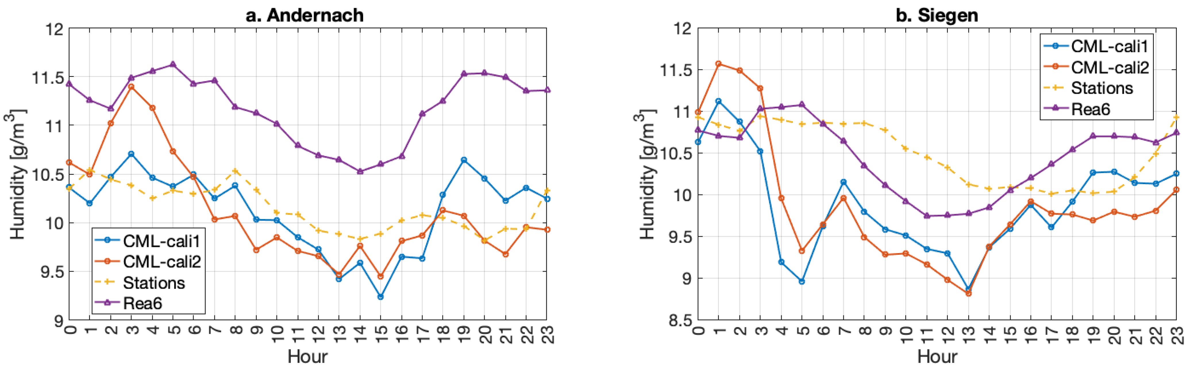
  • Low CML-HO values can result from inaccurate WS-HOm values used for the calculation of RSLom at night. When we calculate the WS-HOm at 2 m AGL, it can be quite different from ~30 AGL humidity, especially at night with low inversion. This seems to improve when we used the second method for calibration (cali2). When looking into the calibration equations (Figure S1), we notice that the slope of the equation is higher during the night, which means that for high elevation CMLs, we will observe lower CML-HO values. When we take one diurnal equation instead of the hourly equations, this effect is improved. This conjecture can explain some of the deviations, but not all of them.
  • An additional factor contributing to low CML-HO at night is an interference that can be caused by near-surface strong stratification of the atmosphere and the interaction between the electromagnetic waves and the changes in the characteristics of the atmosphere layers at night, when the PBLH is closer to the surface and the inversion is approximately at the CML level. This phenomenon was shown in David et al. [40].
  • The strong reduction of the CML-HO at night is observed at many locations and it follows earlier high CML-HO values. For very low inversion layers, the CML could be located within the layer that is characterized by strong gradients of temperature and moisture, and therefore disable the CML-HO retrieval.
We further investigated whether specific CMLs are responsible for low CML-HO values at nighttime. This can happen due to unique environmental or CML characteristics. We examined groups of specific CMLs around several stations and tried to connect the aforementioned effect to some CMLs and the environmental characteristics of the CML, such as length, frequency, terrain elevation and slope, location, land use, topography, and urban effects. The results did not show any significant connections between low CML-HO values at nighttime and any of the aforementioned factors. Nevertheless, while examining the relation between the CMLs and average values, we noticed a possible relation between the low frequencies (lower than 22 GHz) and the low values of CML-HO measured. The relation was not significant for all stations and does not explain the low CML-HO values observed at night. This was concluded after we made another run when we excluded CMLs with frequencies below 22 GHz and obtained similar results.
Beyond the comparison between mean and STD values for the three sources, we analyzed the diurnal cycle of the correlation and the RMSE of CML-HO and Rea6 with respect to WS-HO. The behavior is closely connected to the mean values analysis above. We noticed that there are three times with maximum values of correlation (Figure 2c), which are usually followed by maximum, or close to maximum, values of RMSE (Figure 2d). The (local) minimum correlations were observed at 3 LT and 18 LT, while the maximum correlations were at 12 LT. The Rea6 correlations during the day stay high, around the average (0.85). The minimum and maximum CML-HO-WS-HO correlation times approximately fit the RMSE and STD maximum and minimum times, respectively. When comparing to the Rea6 RMSE and STD patterns, we can notice similarities in the evening and large differences during the night. The similarities may imply that the large differences between CML-HO (and Rea6) and WS-HO could be due to the different level AGL each of them represents. However, the different behavior of the CML-HO RMSE and STD at night (high CML-HO RMSE and STD compared to the Rea6) is not a result of different levels AGL only, and it implies again other factors that affect the CML-HO retrieval at nighttime.

3.3. Inter-Daily Variability

Figure 5a shows a time-series of the hourly values of CML-HO, WS-HO, and Rea6 humidity with hourly rain measurements at the Siegen location during the studied month (June 2018). Figure 5b shows the LWC and PBLH from the ECMWF operational archive and Rea6 (respectively) at the Siegen station location for June 2018. In general, all sources show similar patterns which follow the inter-daily humidity changes. We noticed the connection between the PBLH and the humidity values, such that on days when the PBLH is relatively low, the humidity is high (e.g., 9–10 June 2018) and vice-versa (21 June 2018). However, we notice a systematic negative bias of the CML-HO in comparison to WS-HO. Figure 5 illustrates the typical behavior for many other stations in which we noticed this bias. The reason for the bias could be the aforementioned height differences AGL between the WS-HO and the CML-HO interpolated field, with the CML-HO representing a higher altitude AGL as compared to stations. Based on the general humidity vertical profile, the absolute humidity typically decreases with height, especially at specific atmospheric conditions with a stable atmosphere and low PBLH [37]. We also note that on some days, the CML-HO is much higher. Those days are characterized by rain or dew/fog at the weather station (Figure 5b). This reinforces the aforementioned idea that the CML-HO increase in some points can be associated with air condensation or wet antennae. In general, the algorithm for retrieving the CML-HO neglects events where the attenuation is too strong to retrieve the CML-HO, mostly due to rain. However, when the antenna is covered with a thin layer of water or there are small drops in the air, the attenuation may not be strong enough to be detected as rain. Thus, we still get reasonable CML-HO values below the theoretical maximum value of the Clausius–Clapeyron relation, which connects the temperature and the maximum WV amount the air can hold [41]. In previous studies, we had some instantaneous measurements on a day with a relative high QE [11,12]. In those studies, those outliers were rare and these events were ignored. In the present work, when the temporal resolution is higher and the QE is lower, we must take it into account these limitations and correct them.
We pose two suggestions for correction:
  • Employ the maximum limit for WV in the air as determined by the Clausius–Clapeyron equation. In the current algorithm, we determined the maximum value for true absolute humidity by the maximum value of the temperature for the whole period. If we choose the maximum temperature for a shorter period or instantaneously from a nearby weather station, or even a model, we expect to reduce the error caused by water on the antenna or in the air.
  • Exclude rain events [42,43] and correct wet antenna attenuation (WAA) by the proposed methods for estimate the wet antenna effect [33,34,35,36]. This could be done based on the attenuation itself compared to dry periods, or by additional information from the stations. There are some methods for wet antenna estimation and the results can change between different locations and CMLs characteristics. Alternatively, during the rain events and for several hours afterwards, to allow for complete drying, they can be removed to reduce the errors due to WAA.

4. Discussion and Conclusions

This work focuses on a one month CML-HO at a high spatio–temporal resolution in western Germany. We compared the results to two other data sources: 32 weather stations (WS-HO) and reanalysis at ~30 m AGL in high spatial resolution from the DWD (Rea6).
When comparing CML-HO with WS-HO, we expected to obtain differences between the CML-HO and WS-HO along the diurnal cycle. The diurnal true humidity pattern is strongly influenced by the PBLH, which is largely determined by the inversion height. In the case of low inversion, particularly during night, the observed absolute WS-HO near the surface and under the inversion could be quite different from the CML-HO at the CMLs height, which might be located above the inversion under extreme low inversion conditions—especially at night (tens of meters above the surface). This was shown nicely by mast measurements in the study by Brümmer and Schultze [38] for similar conditions in Germany.
We further elucidate factors that affect the CML-HO retrieval, leading to significant differences with nearby WS-HO: (1) The CMLs are affected by the inversion that is characterized by a sharp vertical air density gradient. This could cause ducting due to the vertical gradient of refractivity that would affect the attenuation [40]. (2) The height AGL can be an important factor. In this study, we assumed the average CML height AGL to be ~30 m; however, the CML height varies and can be lower or even much higher, for example, a CML that connects two higher sites across a valley. Sometimes, the CML towers are positioned at much different elevations so that the CML path can go through different layers of the atmosphere with large gradients in the air humidity. (3) Factors that influence the WV near the CML path, or even the attenuation itself, which have no record that can be checked. For example, it is difficult to relate a factory or a field which can be a source for WV at small scales to the CML-HO retrieval.
While examining the average diurnal cycles of the three humidity observation sources, we noticed good agreement between CML-HO and Rea6 diurnal patterns at most of the daylight hours and at the evening hours, especially with the cali2 method, which uses one equation for calibration for all times. This is likely to be observed as both CML-HO and Rea6 are at the same height (30 m AGL) and both of them represent a spatial mean value (1 km and 6 km grid for the CML-HO and Rea6, respectively) as opposed to the local representativeness of WS-HO point observations. During nighttime hours, the agreement was not clear and was followed by large differences in the RMSE and STD, too. This may imply other factors that may affect the attenuation at night.
The main conclusions of this study are:
  • The best method to retrieve the CML-HO for getting the finest temporal resolution is to calibrate the CMLs calculating RSLm for 24 hour intervals. In addition, when applying one median equation for RSLm for all hours of the day, instead of separate equations for each hour of the day, there is an insignificant improvement, especially in the RMSE at night.
  • Some of the most significant differences between CML-HO and WS-HO can be associated with:
    WAA (water on the antenna) due to rain or condensation.
    LWC, which might cause significant attenuation due to water in the air or WAA.
    PBLH, which affects the humidity vertical profile and might create large differences between the weather station (2 m AGL) and the CML (~30 m AGL) when the inversion layer is closer to the surface, especially at night.
In many cases, this cannot be validated due to the lack of additional data.
  • The height differences between stations and CML can be large. Hence, the verification of CML-HO with respect to WS-HO may lead to differences due to true different humidity at the CML and at the station.
While several challenges are still to be overcome, this work presents a plausible method to monitor humidity in the PBL. The comparison of CML-HO to the reanalysis Rea6 shows that the mean CML-HO closely follows the reanalysis Rea6 values and diurnal pattern during a large period of the day. This stresses the similar representativeness between the CML-HO and Rea6, as opposed to the local representativeness of the WS-HO. This is an encouraging outcome on the way to the assimilation of CML-HO into NWP models, as representativeness is one of the major difficulties in the assimilation of in situ surface observations in mesoscale models.

Supplementary Materials

The following supporting information can be downloaded at: https://www.mdpi.com/article/10.3390/rs14102353/s1, Figure S1: Median humidity vs. Elevation (May 2018, Germany).

Author Contributions

Conceptualization, Y.R., D.R.-E. and P.A.; methodology, Y.R., D.R.-E., C.C. and P.A.; software, Y.R.; validation, Y.R.; formal analysis, Y.R.; investigation, Y.R., D.R.-E. and P.A.; resources, P.A.; data curation, C.C.; writing—original draft preparation, Y.R.; writing—review and editing, D.R.-E.; visualization, Y.R.; supervision, P.A. and D.R.-E.; project administration, Y.R.; funding acquisition, P.A. All authors have read and agreed to the published version of the manuscript.

Funding

This research was funded by the German Research Foundation (DFG) through the project “Integrating Microwave Link Data for Analysis of Precipitation in Complex Terrain: Theoretical Aspects and Hydrometeorological Applications (IMAP)”, project number 254695484.

Institutional Review Board Statement

Not applicable.

Informed Consent Statement

Not applicable.

Data Availability Statement

CML data were provided by Ericsson Germany and are not publicly available. Weather stations data are publicly available from the Climate Data Center of the German Weather Service (https://opendata.dwd.de/climate_environment/CDC/, accessed on 26 March 2022).

Acknowledgments

The authors are grateful to Ericson Germany for providing the CML data, pro bono, for our research. Special thanks are given to the Deutscher Wetterdienst (DWD) for providing free climate station data for Germany. Thanks to I-CHANGE project for partial supportand to Yehuda Alexander for reviewing the manuscript prior to submission.

Conflicts of Interest

The authors declare no conflict of interest. The funders had no role in the design of the study; in the collection, analyses, or interpretation of data; in the writing of the manuscript; or in the decision to publish the results.

Abbreviations

AbbreviationDefinition
AGLAbove Ground Level
AMSLAbove Mean Sea Level
BLBoundary Layer
cali1Calibration method 1: linear equations were calculated for each hour of the day
cali2Calibration method 2: a single linear equation was calculated for all hours of the day together
CMLCommercial Microwave Links
CML-HOCML humidity observations
DWDGermany’s National Meteorological Service, Deutscher Wetterdienst
LCland cover
LWCLiquid Water Content
LTLocal Time
NWPNumerical Weather Prediction
PBLPlanetary Boundary Layer
PBLHPBL heights
QEQuantization Error
Rea6COSMO-REA6 reanalysis
RMSERoot Mean Square Error
RSLReceived Signal Level
STDStandard Deviation
TSLTransmit Signal Level
WAAWet Antenna Attenuation
WS-HOWeather station humidity observations
WVWater Vapor

References

  1. Fabry, F. The Spatial Variability of Moisture in the Boundary Layer and Its Effect on Convection Initiation: Project-Long Characterization. Mon. Weather Rev. 2006, 134, 79–91. [Google Scholar] [CrossRef]
  2. Kunz, M.; Sander, J.; Kottmeier, C. Recent trends of thunderstorm and hailstorm frequency and their relation to atmospheric characteristics in southwest Germany. Int. J. Climatol. 2009, 29, 2283–2297. [Google Scholar] [CrossRef] [Green Version]
  3. Lilly, D.K.; Gal-Chen, T. Mesoscale Meteorology-Theories, Observations and Models; Springer Science & Business Media: Berlin/Heidelberg, Germany, 1983. [Google Scholar]
  4. Toporov, M.; Löhnert, U. Synergy of Satellite- and Ground-Based Observations for Continuous Monitoring of Atmospheric Stability, Liquid Water Path, and Integrated Water Vapor: Theoretical Evaluations Using Reanalysis and Neural Networks. J. Appl. Meteorol. Climatol. 2020, 59, 1153–1170. [Google Scholar] [CrossRef] [Green Version]
  5. Pielke, R.A. Mesoscale Meteorological Modeling, 3rd ed.; International Geophysics Series; Elsevier: Amsterdam, The Netherlands, 2013; ISBN 978-0-12-385237-3. [Google Scholar]
  6. Messer, H.; Zinevich, A.; Alpert, P. Environmental monitoring by wireless communication networks. Science 2006, 312, 713. [Google Scholar] [CrossRef] [Green Version]
  7. Leijnse, H.; Uijlenhoet, R.; Stricker, J.N.M. Rainfall measurement using radio links from cellular communication networks. Water Resour. Res. 2007, 43. [Google Scholar] [CrossRef]
  8. Zinevich, A.; Alpert, P.; Messer, H. Estimation of rainfall fields using commercial microwave communication networks of variable density. Adv. Water Resour. 2008, 31, 1470–1480. [Google Scholar] [CrossRef]
  9. Zinevich, A.; Messer, H.; Alpert, P. Frontal rainfall observation by a commercial microwave communication network. J. Appl. Meteorol. Climatol. 2009, 48, 1317–1334. [Google Scholar] [CrossRef]
  10. Zinevich, A.; Messer, H.; Alpert, P. Prediction of rainfall intensity measurement errors using commercial microwave communication links. Atmos. Meas. Tech. 2010, 3, 1385–1402. [Google Scholar] [CrossRef] [Green Version]
  11. David, N.; Alpert, P.; Messer, H. Technical note: Novel method for water vapour monitoring using wireless communication networks measurements. Atmos. Chem. Phys. 2009, 9, 2413–2418. [Google Scholar] [CrossRef] [Green Version]
  12. Alpert, P.; Rubin, Y. First Daily Mapping of Surface Moisture from Cellular Network Data and Comparison with Both Observations/ECMWF Product. Geophys. Res. Lett. 2018, 45, 8619–8628. [Google Scholar] [CrossRef]
  13. Fencl, M.; Dohnal, M.; Valtr, P.; Grabner, M.; Bareš, V. Atmospheric observations with E-band microwave links–challenges and opportunities. Atmos. Meas. Tech. 2020, 13, 6559–6578. [Google Scholar] [CrossRef]
  14. Pu, K.; Liu, X.; Liu, L.; Gao, T. Water Vapor Retrieval Using Commercial Microwave Links Based on the LSTM Network. IEEE J. Sel. Top. Appl. Earth Obs. Remote Sens. 2021, 14, 4330–4338. [Google Scholar] [CrossRef]
  15. Song, K.; Liu, X.; Gao, T.; Zhang, P. Estimating Water Vapor Using Signals from Microwave Links below 25 GHz. Remote Sens. 2021, 13, 1409. [Google Scholar] [CrossRef]
  16. Ducrocq, V.; Ricard, D.; Lafore, J.-P.; Orain, F. Storm-Scale Numerical Rainfall Prediction for Five Precipitating Events over France: On the Importance of the Initial Humidity Field. Weather Forecast. 2002, 17, 1236–1256. [Google Scholar] [CrossRef]
  17. Rostkier-Edelstein, D.; Hacker, J.P. The Roles of Surface-Observation Ensemble Assimilation and Model Complexity for Nowcasting of PBL Profiles: A Factor Separation Analysis. Weather Forecast. 2010, 25, 1670–1690. [Google Scholar] [CrossRef]
  18. Ha, S.-Y.; Snyder, C. Influence of Surface Observations in Mesoscale Data Assimilation Using an Ensemble Kalman Filter. Mon. Weather Rev. 2014, 142, 1489–1508. [Google Scholar] [CrossRef] [Green Version]
  19. Bonafoni, S.; Biondi, R.; Brenot, H.; Anthes, R. Radio occultation and ground-based GNSS products for observing, understanding and predicting extreme events: A review. Atmos. Res. 2019, 230, 104624. [Google Scholar] [CrossRef]
  20. Ho, S.; Anthes, R.A.; Ao, C.O.; Healy, S.; Horanyi, A.; Hunt, D.; Mannucci, A.J.; Pedatella, N.; Randel, W.J.; Simmons, A.; et al. The COSMIC/FORMOSAT-3 Radio Occultation Mission after 12 Years: Accomplishments, Remaining Challenges, and Potential Impacts of COSMIC-2. Bull. Am. Meteorol. Soc. 2020, 101, E1107–E1136. [Google Scholar] [CrossRef] [Green Version]
  21. Andersson, E.; Hólm, E.; Bauer, P.; Beljaars, A.; Kelly, G.A.; McNally, A.P.; Simmons, A.J.; Thépaut, J.-N.; Tompkins, A.M. Analysis and forecast impact of the main humidity observing systems. Q. J. R. Meteorol. Soc. 2007, 133, 1473–1485. [Google Scholar] [CrossRef]
  22. Geer, A.J.; Baordo, F.; Bormann, N.; Chambon, P.; English, S.J.; Kazumori, M.; Lawrence, H.; Lean, P.; Lonitz, K.; Lupu, C. The growing impact of satellite observations sensitive to humidity, cloud and precipitation: Impact of Satellite Humidity, Cloud and Precipitation Observations. Q. J. R. Meteorol. Soc. 2017, 143, 3189–3206. [Google Scholar] [CrossRef]
  23. Gustafsson, N.; Janjić, T.; Schraff, C.; Leuenberger, D.; Weissmann, M.; Reich, H.; Brousseau, P.; Montmerle, T.; Wattrelot, E.; Bučánek, A.; et al. Survey of data assimilation methods for convective-scale numerical weather prediction at operational centres. Q. J. R. Meteorol. Soc. 2018, 144, 1218–1256. [Google Scholar] [CrossRef] [Green Version]
  24. Chwala, C.; Kunstmann, H. Commercial microwave link networks for rainfall observation: Assessment of the current status and future challenges. Wiley Interdiscip. Rev. Water 2019, 6, e1337. [Google Scholar] [CrossRef] [Green Version]
  25. Dee, D.P.; Uppala, S.M.; Simmons, A.J.; Berrisford, P.; Poli, P.; Kobayashi, S.; Andrae, U.; Balmaseda, M.A.; Balsamo, G.; Bauer, P.; et al. The ERA-Interim reanalysis: Configuration and performance of the data assimilation system. Q. J. R. Meteorol. Soc. 2011, 137, 553–597. [Google Scholar] [CrossRef]
  26. Hersbach, H.; Bell, B.; Berrisford, P.; Hirahara, S.; Horányi, A.; Muñoz-Sabater, J.; Nicolas, J.; Peubey, C.; Radu, R.; Schepers, D.; et al. The ERA5 global reanalysis. Q. J. R. Meteorol. Soc. 2020, 146, 1999–2049. [Google Scholar] [CrossRef]
  27. Liebe, H.J. An updated model for millimeter wave propagation in moist air. Radio Sci. 1985, 20, 1069–1089. [Google Scholar] [CrossRef] [Green Version]
  28. van Vleck, J.H. The Absorption of Microwaves by Uncondensed Water Vapor. Phys. Rev. 1947, 71, 425–433. [Google Scholar] [CrossRef]
  29. Rubin, Y. A Novel Approach for High Resolution Humidity Mapping Based on Cellular Net-Work Data. Master’s Thesis, Tel-Aviv University, Tel-Aviv, Israel, 2018. [Google Scholar]
  30. David, N.; Sendik, O.; Rubin, Y.; Messer, H.; Gao, H.O.; Rostkier-Edelstein, D.; Alpert, P. Analyzing the ability to reconstruct the moisture field using commercial microwave network data. Atmos. Res. 2019, 219, 213–222. [Google Scholar] [CrossRef]
  31. Cressman, G.P. An Operational Objective Analysis System. Mon. Weather Rev. 1959, 87, 367–374. [Google Scholar] [CrossRef]
  32. Wilks, D.S. Statistical Methods in the Atmospheric Sciences, 3rd ed.; International Geophysics Series; Academic Press: Oxford Waltham, MA, USA, 2011; ISBN 978-0-12-385022-5. [Google Scholar]
  33. Leijnse, H.; Uijlenhoet, R.; Stricker, J.N.M. Microwave link rainfall estimation: Effects of link length and frequency, temporal sampling, power resolution, and wet antenna attenuation. Adv. Water Resour. 2008, 31, 1481–1493. [Google Scholar] [CrossRef]
  34. Ostrometzky, J.; Raich, R.; Bao, L.; Hansryd, J.; Messer, H. The Wet-Antenna Effect—A Factor to be Considered in Future Communication Networks. IEEE Trans. Antennas Propag. 2018, 66, 315–322. [Google Scholar] [CrossRef]
  35. Fencl, M.; Valtr, P.; Kvicera, M.; Bares, V. Quantifying Wet Antenna Attenuation in 38-GHz Commercial Microwave Links of Cellular Backhaul. IEEE Geosci. Remote Sens. Lett. 2019, 16, 514–518. [Google Scholar] [CrossRef]
  36. David, N.; Harel, O.; Alpert, P.; Messer, H. Study of attenuation due to wet antenna in microwave radio communication. In Proceedings of the 2016 IEEE International Conference on Acoustics, Speech and Signal Processing (ICASSP), Shanghai, China, 20–25 March 2016; pp. 4418–4422. [Google Scholar]
  37. Stull, R.B. An Introduction to Boundary Layer Meteorology; Atmospheric Sciences Library; Kluwer Academic Publ: Dordrecht, The Netherlands; Boston, MA, USA; London, UK, 1988; ISBN 978-90-277-2768-8. [Google Scholar]
  38. Brümmer, B.; Schultze, M. Analysis of a 7-year low-level temperature inversion data set measured at the 280 m high Hamburg weather mast. Meteorol. Z 2015, 24, 481–494. [Google Scholar] [CrossRef]
  39. Haikin, N.; Galanti, E.; Reisin, T.G.; Mahrer, Y.; Alpert, P. Inner Structure of Atmospheric Inversion Layers over Haifa Bay in the Eastern Mediterranean. Bound.-Layer Meteorol. 2015, 156, 471–487. [Google Scholar] [CrossRef]
  40. David, N.; Gao, H.O. Using Cellular Communication Networks To Detect Air Pollution. Environ. Sci. Technol. 2016, 50, 9442–9451. [Google Scholar] [CrossRef] [PubMed]
  41. Warner, T.T. Numerical Weather and Climate Prediction; Cambridge University Press: Cambridge, UK, 2011; ISBN 978-0-521-51389-0. [Google Scholar]
  42. Graf, M.; Chwala, C.; Polz, J.; Kunstmann, H. Rainfall estimation from a German-wide commercial microwave link network: Optimized processing and validation for 1 year of data. Hydrol. Earth Syst. Sci. 2020, 24, 2931–2950. [Google Scholar] [CrossRef]
  43. Polz, J.; Chwala, C.; Graf, M.; Kunstmann, H. Big commercial microwave link data: Detecting rain events with deep learning. In Proceedings of the 22nd EGU General Assembly, Online, 4–8 May 2020. [Google Scholar]
Figure 1. (left) A map of the research domain. The CMLs are indicated by black lines and the weather stations’ locations by their number in white circles (Stations list, Table 1). The CMLs are located in a larger domain of ~40 km around the study domain. For the topographic map of the region and the research domain in it see right panel (right, black square). Points B, S, and F represent Bonn, Siegen, and Frankfurt, respectively (Stations 15, 26, and 9 in Table 1, respectively).
Remotesensing 14 02353 g001
Figure 2. Mean correlations (a), RMSE (b), mean absolute humidity values (c), and STD (d) for all stations with full available data when applying 24 h intervals for calibration and an effective radius for interpolation of 40 km (32 stations, mean elevation 271 m, STD-165 m). Two runs were performed: (1) with different equations for calibration at each hour of the day (blue, CML-HO-cali1) and (2) with the same equation for calibration for all the hours (red, CML-HO-cali2, see methodology). Results that refer to Rea6 are in yellow and those referring to weather stations (WS-HO) are in purple.
Remotesensing 14 02353 g002
Figure 3. Mean diurnal PBLH (in black), LWC (red), and LWC change (dashed red) for June 2018. Data were analyzed for all stations based on ECMWF operational archive (LWC) and PBLH from Rea6.
Remotesensing 14 02353 g003
Figure 4. Diurnal CML-HO (CML-cali1/2), WS-HO (Stations), and Rea6 for two stations with a different CML-HO behavior. (a) A station with high humidity values at night, as observed at the WS, that gradually decrease until the morning. At this station, there is no significant decrease at night, and a similar pattern to the Rea6 is observed during the day. (b) A station with low CML-HO values as compared to WS-HO at night. The same calibration equation for all hours was applied (red, cali2). Rea6 is yellow and WS-HO is purple.
Remotesensing 14 02353 g004
Figure 5. (a) Upper panel: hourly humidity observations for June 2018 from CML, stations, and Rea6 (scale on left), as well as hourly precipitation (light blue, rain scale on right in mm/h) at the Siegen station. (b) LWC (kg/kg in red) and PBLH (meters, in black) from the ECMWF operational archive and Rea6 (respectively) for June 2018.
Remotesensing 14 02353 g005
Table 1. A list of the weather stations and their elevation AMSL in meters.
NumberNameElevation [m]
1Berleburg, Bad-Stenzel610
2Andernach75
3Blankenrath417
4Bonn-Roleber159
5Büchel (Flugplatz)477
6Burgwald-Bottendorf293
7Dillenburg314
8Frankfurt/Main100
9Frankfurt/Main-Westend124
10Gießen/Wettenberg203
11Hilgenroth295
12Hümmerich328
13Kahl/Main107
14Kleiner Feldberg/Taunus826
15Köln-Bonn92
16Lennestadt-Theten286
17Löhnberg-Obershausen230
18Marburg-Biedenkopf187
19Marienberg, Bad547
20Montabaur265
21Nauheim, Bad149
22Neuenahr, Bad-Ahrweiler111
23Neunkirchen-Seelscheid-Krawinkel195
24Reichshof-Eckenhagen350
25Remscheid-Lennep345
26Siegen (Kläranlage)229
27Waldems-Reinborn380
28Wiesbaden-Auringen263
29Nastätten268
30Runkel-Ennerich168
31Offenbach-Wetterpark119
32Meinerzhagen-Redlendorf380
Table 2. Averaged correlation, RMSE, mean and STD based on the cali2 method and comparisons at all the WSs locations. A comparison between reanalysis (Rea6) and CML-HO (cali2) based on the comparison to WS-HO. The values represent the averages for the whole period (June 2018) for each hour of the day, separately. The number in the first row (SUM#) indicates on the better results for each observation source. Other rows summarized the mean for all the hours (second row) and for different parts of the day (numbers refer to the local time). The better method, i.e., CML or Rea6, is indicated in blue.
HourCorr_CML_StationsCorr_Rea6S_StationsRMSE_CML_StationsRMSE_Rea6_StationsMean_StationsMean_CMLMean_Rea6STD_StationsSTD_CMLSTD_Rea6
SUM#717618 1212 618
MEAN0.840.851.581.4910.7410.1210.042.212.262.29
MEAN 9-170.870.841.531.5510.499.769.782.382.242.29
MEAN 18-80.820.861.611.4610.8910.3410.192.102.272.29
MEAN 6-21 (DAYLIGHT)0.8530.8521.591.5410.679.859.892.312.252.30
MEAN 22-5 (NIGHT)0.810.861.561.4010.8910.6710.332.012.262.27
Publisher’s Note: MDPI stays neutral with regard to jurisdictional claims in published maps and institutional affiliations.

