Article

Dynamic Range Compression Self-Adaption Method for SAR Image Based on Deep Learning

1
The Radar Research Laboratory, Beijing Institute of Technology, Beijing 100081, China
2
Beijing Institute of Technology Chongqing Innovation Center, Chongqing 401135, China
*
Author to whom correspondence should be addressed.
Remote Sens. 2022, 14(10), 2338; https://doi.org/10.3390/rs14102338
Submission received: 31 March 2022 / Revised: 2 May 2022 / Accepted: 10 May 2022 / Published: 12 May 2022
(This article belongs to the Special Issue Distributed Spaceborne SAR: Systems, Algorithms, and Applications)

Abstract

:
The visualization of synthetic aperture radar (SAR) images involves the mapping of high dynamic range (HDR) amplitude values to gray levels for lower dynamic range (LDR) display devices. This dynamic range compression process determines the visibility of details in the displayed result. It therefore plays a critical role in remote sensing applications. There are some problems with existing methods, such as poor adaptability, detail loss, imbalance between contrast improvement and noise suppression. To effectively obtain the images suitable for human observation and subsequent interpretation, we introduce a novel self-adaptive SAR image dynamic range compression method based on deep learning. Its designed objective is to present the maximal amount of information content in the displayed image and eliminate the contradiction between contrast and noise. Considering that, we propose a decomposition-fusion framework. The input SAR image is rescaled to a certain size and then put into a bilateral feature enhancement module to remap high and low frequency features to realize noise suppression and contrast enhancement. Based on the bilateral features, a feature fusion module is employed for feature integration and optimization to achieve a more precise reconstruction result. Visual and quantitative experiments on synthesized and real-world SAR images show that the proposed method notably realizes visualization which exceeds several statistical methods. It has good adaptability and can improve SAR images’ contrast for interpretation.

Graphical Abstract

1. Introduction

As one of the main sources of remote sensing, synthetic aperture radar (SAR) has the all-day and all-weather observation capability [1]. Therefore, the SAR image plays an important role in remote sensing applications, including disaster monitoring, resource exploration, target detection, etc. However, the pixel values of SAR images have a high dynamic range, it is difficult to present the maximal amount of information content in the displayed image, and it is unsuitable for human observation. This problem also affects the subsequent intelligent interpretation. Hence, the visualization of SAR images plays a crucial role in remote sensing applications.
In order to realize SAR image visualization, many dynamic range compression algorithms are proposed. Generally speaking, the HDR compression techniques can be roughly divided into two types: filter based and transfer function based. However, the filter-based techniques are fundamentally improper for SAR image dynamic range reduction tasks. This is because for SAR images, filter-based HDR compression techniques actually perform a high boost filtering on the input SAR images. Although the contrast can be enhanced significantly by high boost filtering, the ranks of the intensity levels are destroyed in the output image. The loss of intensity ranks may cause the visual reversal of brightness. It means that an object with higher reflectance ratio may appear darker than the other objects with a lower reflectance ratio. This may bring unpredictable consequences to the applications such as object detection and classification, image analysis, and so on. Therefore, an important criterion for SAR image dynamic range compression is to preserve the intensity ranks in the output image. It is necessary to preserve the structure information of original SAR images.
The rank preservation property is one of the most significant advantages of the transfer function-based HDR compression techniques. This kind of techniques can reshape the output histogram and at the same time the rank of intensity levels can be preserved. A typical histogram based dynamic range compression algorithm is the well-known histogram equalization HE [2] and its variants. But the overall brightness of images processed by HE is too high to damage details and noise is enlarged, therefore adaptive histogram equalization (AHE) [3] was proposed. AHE divides images into sub-regions, then it performs histogram equalization on each sub-region. But when a sub-region contains similar pixel values, the noise in this area will be further enlarged. For this reason, an adaptive histogram equalization method based on contrast limitation (CLAHE) [4] is proposed. By presetting a threshold value, the histogram is clipped to avoid excessive contrast amplification. In addition, there are some image enhancement methods based on Retinex [5] theory. Single-scale Retinex (SSR) [6] struggles to achieve the balance between good contrast enhancement and detailed structure information preservation. For this reason, multi-scale Retinex (MSR) was proposed [7], but it will generate halo in areas with a large discrepancy of brightness. Besides, the details in bright areas of its results will not be significantly improved. Other dynamic range compression algorithms are based on S-type function mapping, such as Gamma correction [8] and logarithmic transformation [9]. They both have poor adaptability and rely on manual parameter selection. To sum up, these traditional methods are fast in calculation, but poor in performance, unable to adjust the contrast of different images adaptively, and have the problem of missing detailed structure information, which brings challenges to subsequent image interpretations.
Then, in terms of the above problems, some improved methods have been put forward. Zhijiang Li et al. [10] proposed a new SAR image high dynamic range compression and pseudo-color processing algorithm based on Retinex. Gaussian filtering was used to divide the SAR images into uniform parts and detail parts, and then the detail parts were remapped to obtain the final compressed images. Satoshi Hisanaga et al. [11,12] proposed a dynamic range compression algorithm for SAR images based on classification and fusion respectively. Firstly, the algorithm eliminated the little difference between pixels to achieve the effect of noise suppression through neighborhood nonlinear processing. Then, a Laplacian filter was used to roughly classify the target region with high pixel values. The k-mean clustering algorithm and region growth algorithm were used to perform fine classification. Finally, linear equalization processing with brightness limitation was carried out for various regions, and the final visual image could be obtained by fusion of the processed results. The character of this algorithm is that the target and the background were separated, so the details of the target area were saved effectively. However, the fusion results of the algorithm were prone to generating obvious classification boundaries. Aakash Upadhyay et al. [13] proposed a SAR image adaptive enhancement algorithm after compression. Firstly, the Detail Preserving Anisotropic Diffusion algorithm (DPAD) was used to separate speckle noise and the edge details in the images to realize noise suppression. The edge details were enhanced and superimposed with other parts to obtain the final processing results. In the algorithm, JSEG (J-segmentation) was used to extract edge details, and the linear contraction function was used to enhance the edge details adaptively. This algorithm could not only suppress the speckle noise, but also enhance the details in the images. To sum up, these improved methods can overcome the existing problems to a certain extent, but in practical applications, they are too time-consuming. Furthermore, they achieved good performance in specific scenes and had their own limitations when processing SAR images.
For the inherent noise of SAR images, various model-based methods have been developed to suppress speckle noise, such as adaptive local statistical filtering methods [14], wavelet-based methods [15], sparse representation methods [16], block match and 3-D filter (BM3D) algorithm [17], and the total variation(TV) method [18]. However, traditional algorithms still have difficulty in distinguishing details from noise, which usually results in noise residuals or over-smoothing effects. Researchers have also explored the application of deep networks to SAR image despeckling. SAR-CNN [19] is the first network based on deep learning that realizes SAR image despeckling through 17-layer CNNs. SAR-DRN [20] is a lightweight dilated residual network for SAR image despeckling, which introduced residual structure and dilation convolution to maintain performance while reducing training complexity. In addition, HDRANet [21] employed the skip connection and the dilation convolution to make full use of contextual information. It also introduced attention mechanism to emphasize effective features and suppress useless features. In our paper, we aim to avoid the amplification of noise. In other words, noise suppression is taken into consideration rather than despeckling. By referring to these despeckling methods [22,23], our proposed dynamic range compression method can realize visualization without amplifying the existing noise.
In recent years, deep learning has achieved great success in the field of low-level image processing [23,24,25]. End-to-end networks and GANs [26] have been widely used as powerful tools, including image super-resolution [27,28], image denoising [29] and image-to-image conversion [30,31]. Yan et al. [32] took the first step in exploring the use of CNN for image editing. Some CNN-based methods, such as LLCNN [33], a convolutional neural network for low-light image enhancement, can handle brightness and contrast enhancement. Lore et al. [34] proposed a deep learning-based approach to adaptively enhance and denoise images captured in low-light environments, i.e., LLNet, directly using the existing deep neural network architecture (i.e., stack sparse denoising auto encoder) to establish the relationship between low-light images and corresponding enhanced and denoised images. Experimental results show that the method based on deep learning is suitable for low-light image enhancement. Because of the successful exploration in the field of optical images for low-light images enhancement, this paper will explore the use of CNN for SAR image dynamic range compression tasks.
As far as we know, the SAR image dynamic range compression based on deep learning has not been widely studied, so we propose a framework for SAR image visualization by learning the mapping from original SAR images with high dynamic range to ground truth. The main contributions of this work are as follows: (1) To realize SAR images visualization adaptively, we propose a dynamic range compression framework based on CNN. This framework improves the image contrast, suppresses noise and preserves details effectively by decomposition and fusion; (2) In order to eliminate the contradiction between contrast and noise, a bilateral feature enhancement module is designed. It can build a more effective semantic feature description of SAR images by remapping high and low frequency features of SAR images; (3) To achieve a more precise reconstruction result, a feature fusion module is designed. It can integrate bilateral features and further optimize feature description by fine-tuning and selecting useful responses; and (4) To testify the validation of the proposed framework, visual and quantitative experiments are conducted on synthesized and real-world SAR images. The results show that our proposed framework notably improves contrast with better preserving details and suppressing noise, which outperforms several traditional dynamic range compression methods.
The rest of this paper is organized as follows: In Section 2, the proposed decomposition-fusion framework for SAR visualization is introduced in detail; in Section 3, implementation details of experiments are introduced, visual results are presented and quantitative analysis is carried out; in Section 4, we discuss the success of the proposed method and some additional notes; finally, conclusions are drawn in Section 5.

2. Proposed Method

In this section, firstly, we give an overview of the proposed decomposition-fusion framework. Then, the modules in the proposed framework are illustrated respectively. Finally, we introduce the hybrid loss function that we designed.

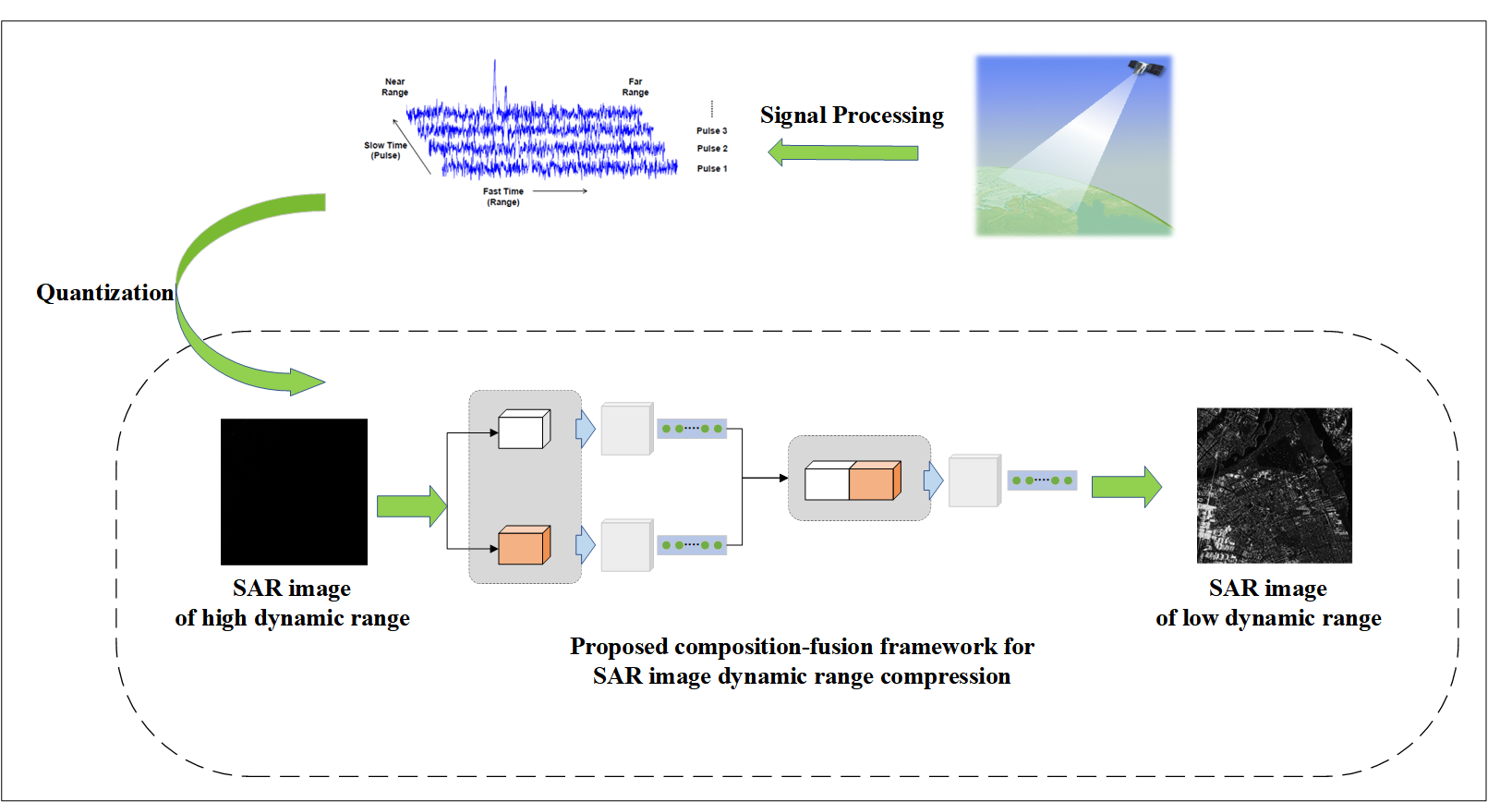
2.1. Overview of Proposed Decomposition-Fusion Framework

The proposed framework comprises two adjacent modules: a bilateral feature enhancement module and a feature fusion module. One is for high and low frequency features remapping and the other is for bilateral features integration.
As shown in Figure 1, the inputs of dimension H × W × 3 are mapped into feature space by the bilateral feature enhancement module. Then, the bilateral feature maps are passed through the feature fusion module to be integrated. After scaling to the original dimension of H × W × 3, visualized images are obtained. Moreover, by minimizing a metric between generated images and ground truth, the network is trained and updated.

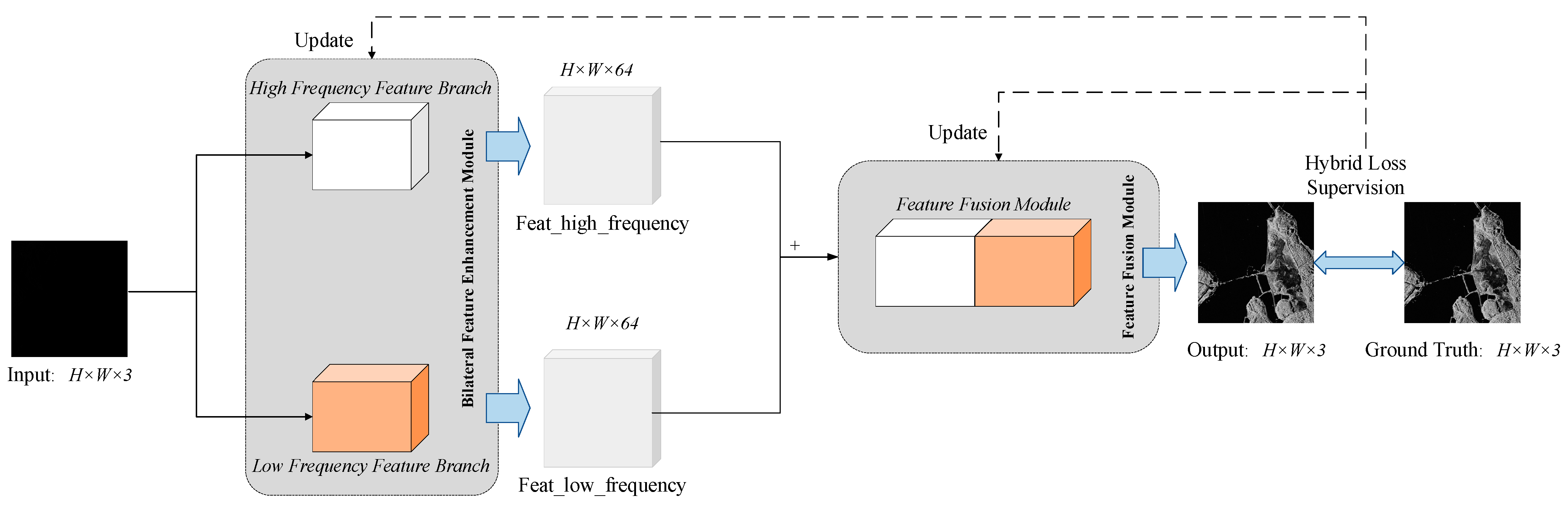
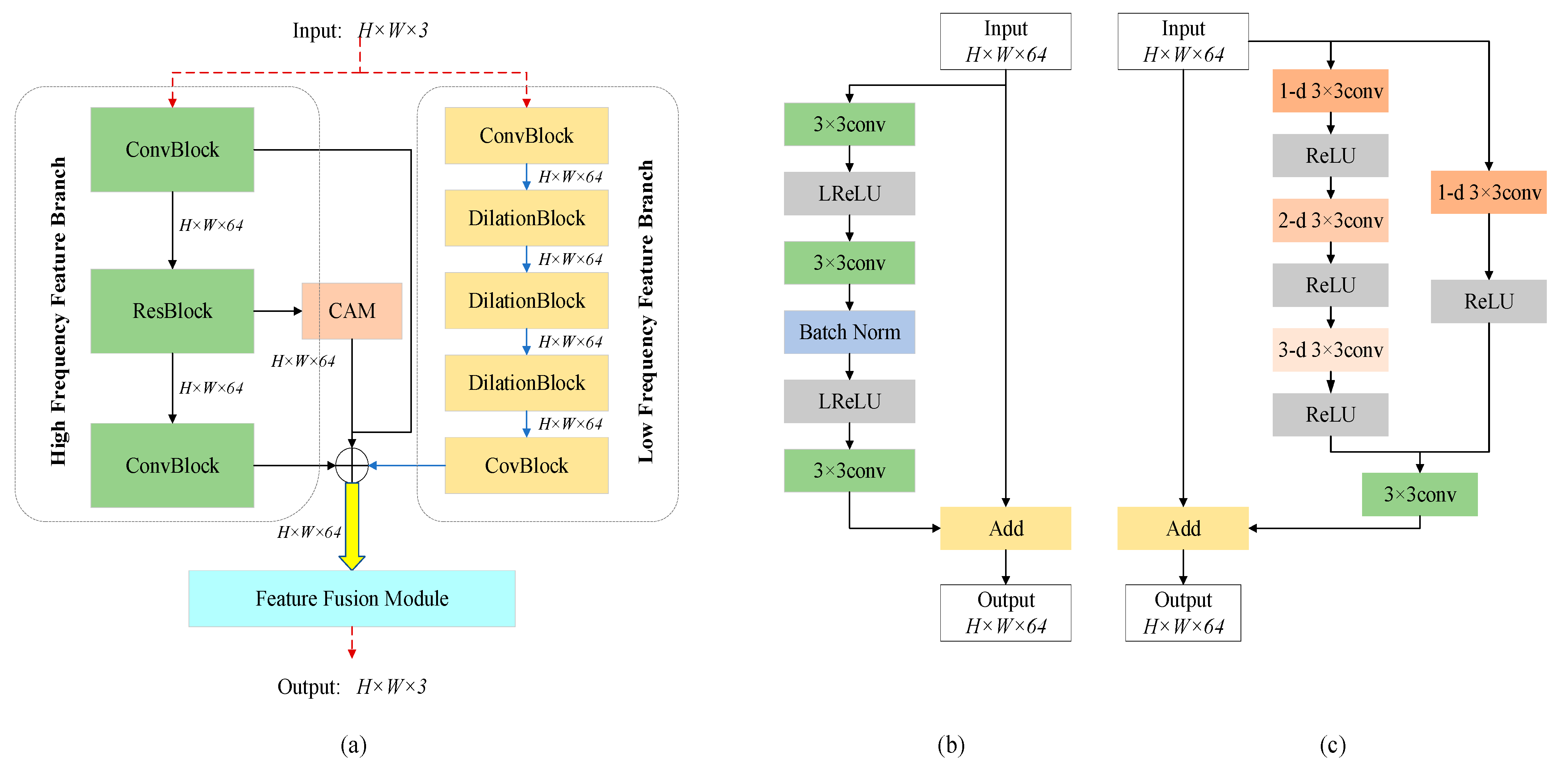
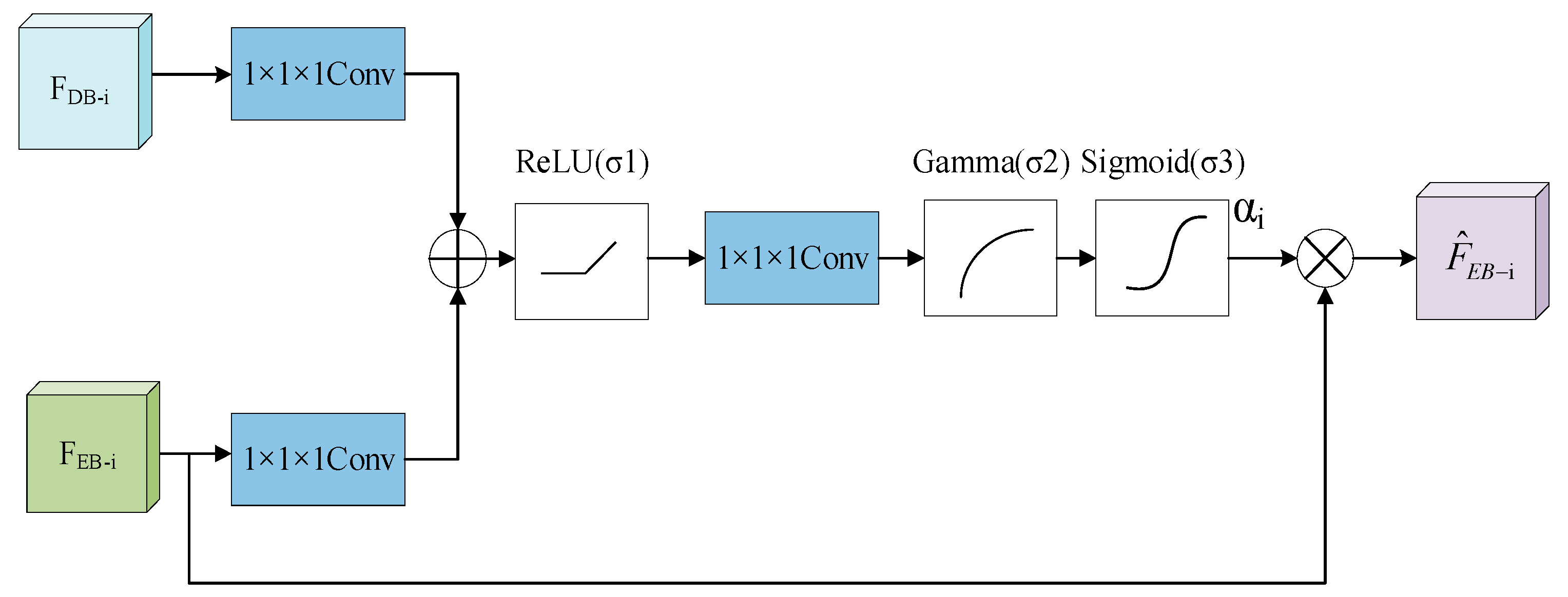
2.2. Bilateral Feature Enhancement Module

In general, optical low-light image enhancement tasks usually utilize networks to remap pixel values directly. However, direct mapping causes noise to increase along with contrast. In order to eliminate the contradiction between contrast and noise, a bilateral feature enhancement module is proposed. As shown in Figure 2a, two independent feature extraction branches are used to suppress noise and enhance contrast by remapping respectively. This ensures that features in each branch are valid and would not interfere with each other. Finally, the output features of dimension H × W × 64 from the two branches are added together as an input of feature fusion module presented in Section 2.3. The two independent feature extraction branches: high frequency feature branch and low frequency feature branch, will be separately introduced below.

2.2.1. High Frequency Feature Branch

DnCNN has demonstrated that employing residual learning and convolution layers can endow a strong ability of denoising. In Figure 2a, the left part of the bilateral feature enhancement module is the high frequency feature branch.
First, the input of dimension H × W × 3 is mapped into feature space by a ConvBlock. A ResBlock is followed, as shown in Figure 2b. It consists of 3 × 3 convolution, batch normalization and Leaky ReLU [35], with appropriate zero padding to ensure that the output of each layer has the same dimension as the input image. After a series of cascaded operation, the feature map is added with the input feature of dimension H × W × 64 to integrate more spatial information. Then, the feature map of ResBlock is fed into a channel attention module (CAM), which is designed to highlight important features and reduce computational redundancy. Finally, the outputs of CAM and these two ConvBlocks are added together as the high frequency feature branch’s output of dimension H × W × 64.
The high frequency feature branch builds a preliminary remap of high frequency features and suppresses noise.

2.2.2. Low Frequency Feature Branch

In the CNN models, more context information is usually obtained by enlarging the receptive field, which is mainly achieved by increasing the size of the filters or stacking the convolution layers. However, these operations undoubtedly increase the number of parameters and the complexity of the model. In Figure 2a, we cascade hybrid dilation convolution blocks to extract and remap the low frequency features from the input image of dimension H × W × 3.
By employing dilation convolution, it can effectively enlarge the receptive field while keeping the filter size and network depth unchanged. The structure of DilationBlock is shown in Figure 2c. First, we adopt a channel-split strategy to avoid channel-wise interferences. Specially, two paralleled convolution branches are split into two 64/2 feature maps. In the left branch, the dilation rates are set to 1, 2, and 3 respectively to avoid grid artifacts [36]. The right branch consists of a 3 × 3 convolution and a ReLU. The output feature maps of two branches are added and adjusted by a 3 × 3 convolution to obtain an H × W × 64 feature map. Then, the input feature of dimension H × W × 64 is added to integrate more spatial information. After two ConvBlocks and three DilationBlocks, the feature map of dimension H × W × 64 is added with that of the high frequency feature branch for feature fusion.
The low frequency feature branch builds a preliminary remap of low frequency features and improves overall contrast.

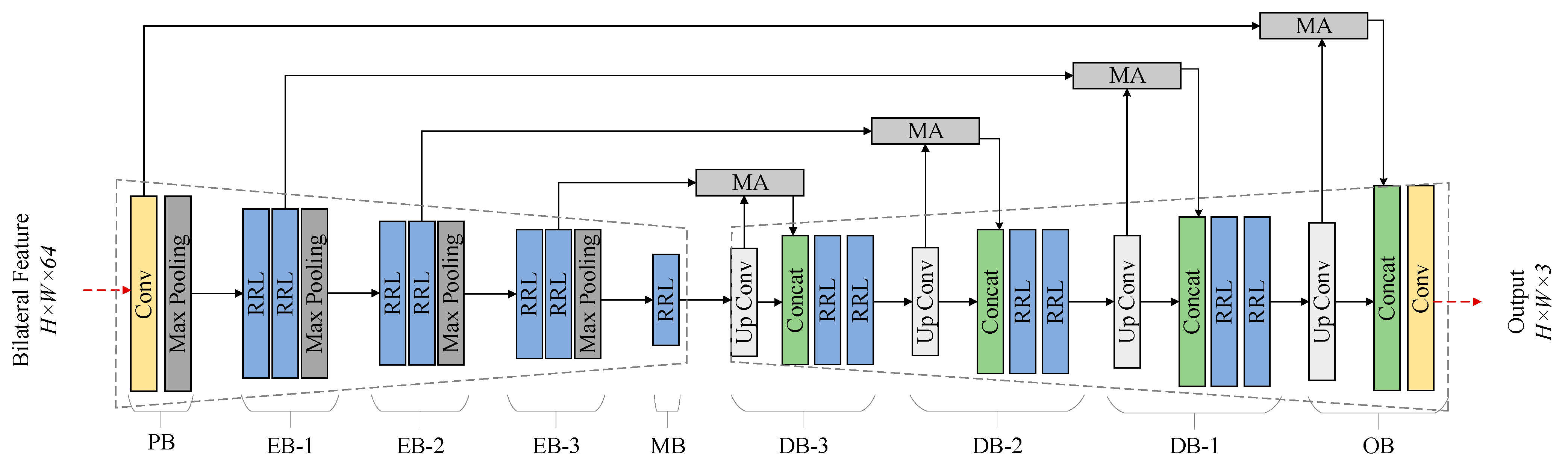
2.3. Feature Fusion Module

To fuse remapped high and low frequency features in a more effective way, a feature fusion module is proposed. For the features generated from bilateral feature enhancement module, we employ a symmetric encoder-decoder network to integrate and optimize them. This structure allows details to be captured at different scales with the increase of network depth. The encoder part is utilized to integrate different values of bilateral features, and the decoder part is used for retrieving and reconstructing features.
The feature fusion module consists of a preprocessing block (PB), three encoder blocks (EB), a middle block (MB), three decoder blocks (DB), and an output block (OB). The architecture is presented in Figure 3.
First, the input of dimension H × W × 64 is down-sampled to a certain size by PB. Then, the feature maps with different scales pass through a series of cascaded EBs. Each EB is made up of a max pooling and two residual recursive learning (RRL) units described in Section 2.3.1. Each EB produces a tensor of the feature map with double the channels. The MB is followed. It resizes the feature map in preparation for decoding. After a series of symmetrical DBs and the OB, the result of the visualized image is obtained.
Moreover, the skip connection is introduced to fuse the shallow and deep features between PB and OB, EB-1 and DB-1, EB-2 and DB-2, EB-3 and DB-3, respectively. Before the shallow features passed to the corresponding blocks, a muti-scale attention mechanism (MA) described in Section 2.3.2 is used to enhance useful features to obtain an effect of further noise suppression. Hence, with the skip connections and the MA, the information lost during the maximum pooling operation can be restored and a larger amount of contextual information is integrated to compensate the more genuine details.

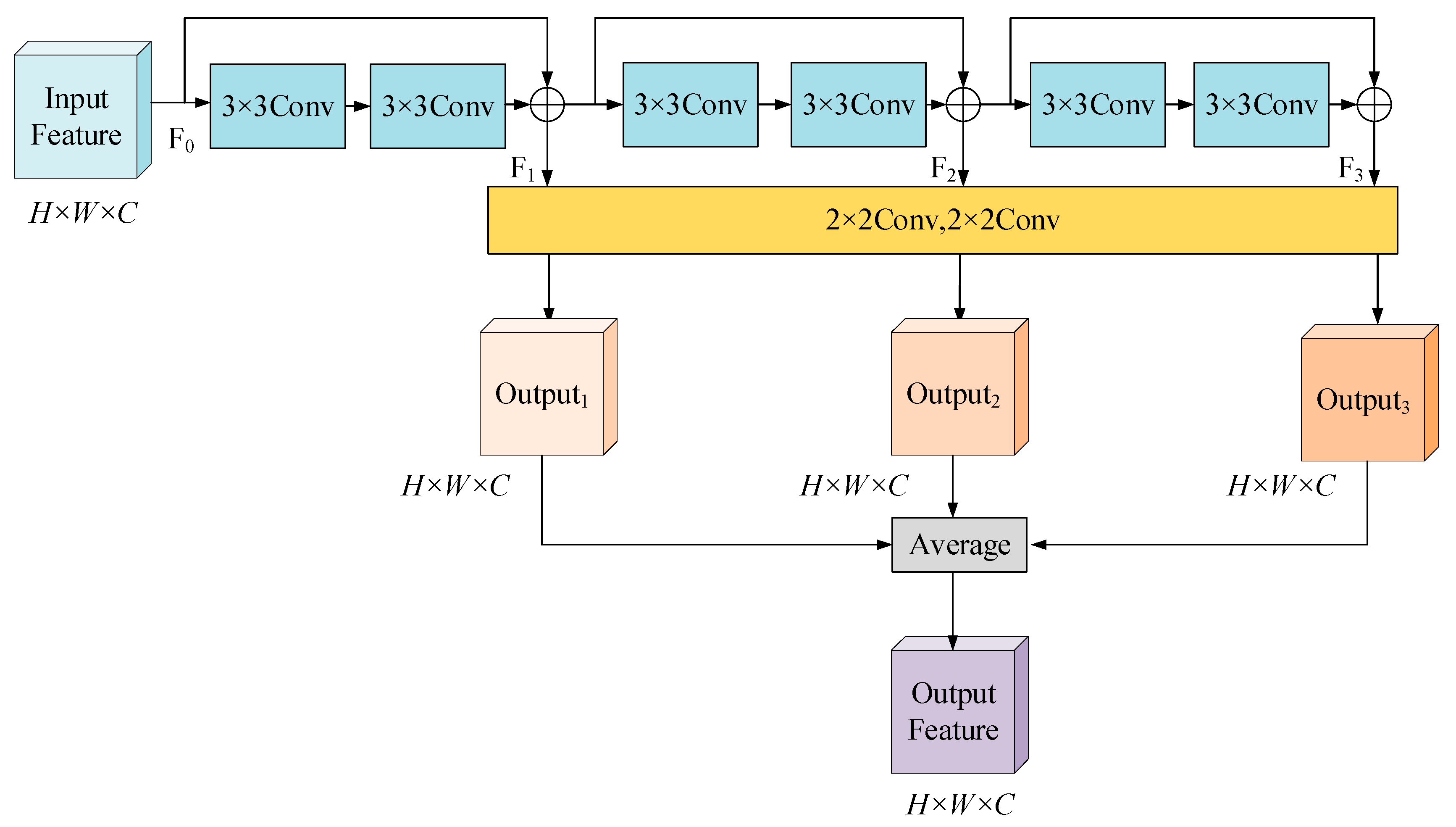
2.3.1. Residual Recursive Learning Unit

To enhance feature extraction, we introduced the residual recursive learning unit (RRL) in the EBs, MB and DBs. Different from the subblocks of the traditional UNet, the RRL combines the residual blocks and recursive structure, as presented in Figure 4.
An RRL unit can optimize the input feature representation. First, feature maps after each recursion contain previous information. It utilizes a very large context through extracting features recursively compared to ordinary serial convolution. Second, all recursions are supervised. By combining all feature maps resulting from different levels of recursions, it can deliver a more accurate final prediction map. The optimal feature representation is automatically learned during training.
Let the input feature of dimension H × W × C be F0. It is the output of RRL’s previous layer in the feature fusion module. The output Fi of each residual block in the recursive relationship can be expressed as:
F i = δ ( δ ( F i 1 W 3 × 3 ) W 3 × 3 ) + F i 1 ,
where, δ is the activation function LeakyReLU, ∗ is the convolution operation, and W is the weight of the current convolution kernel.
The results of each residual block are reconstructed by two 2 × 2 convolution kernels:
O u t p u t i = δ ( W 2 × 2 F i ) ,
We directly pad zeros before each convolution to make sure that feature maps of the middle layers have the same size as the input image. Their dimensions are H × W × C.
In order to avoid the difficulty of convergence caused by recursion and to select the optimal feature, the outputs of residual recursive blocks are supervised by weighting them to obtain the final output feature of dimension H × W × C:
O F = 1 3 i = 1 3 O u t p u t i ,

2.3.2. Multi-Scale Attention Mechanism
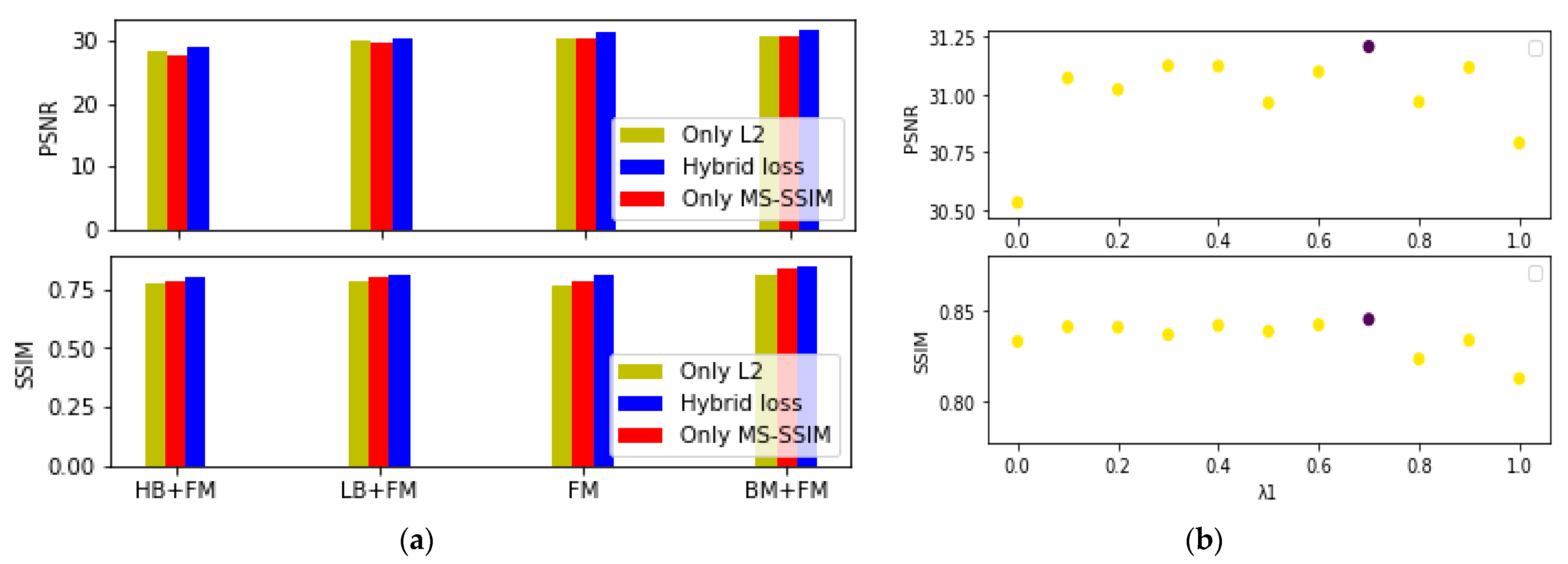
In order to highlight salient features that are passed through the skip connections, a multi-scale attention (MA) mechanism is incorporated into the encoder-decoder architecture, as presented in Figure 5. Information extracted from the coarse scale is used to disambiguate irrelevant and noisy responses in skip connections. This is performed right before the concatenation operation to merge relevant activations only.
Specially, each feature of DB-i is used for each feature of EB-i to determine focus regions. MA helps generate attention coefficients αi to prune lower feature responses before concatenation. The attention coefficients are formulated as follows:
α i = σ 3 ( σ 2 ( σ 1 ( F D B i W 1 × 1 × 1 + F E B i W 1 × 1 × 1 ) W 1 × 1 × 1 ) ) ,
σ 1 ( x ) = max ( 0 , x ) ,
σ 2 ( x ) = x γ ,
σ 3 ( x ) = 1 1 + e x ,
where, ∗ is the convolution operation, W is the weight of the current convolution kernel, σ1 is ReLU operation, σ2 is Gamma correction, σ3 is sigmoid operation, γ is the Gamma correction coefficient, x is the feature map.
First, the linear transformations are computed using channel-wise 1×1×1 convolutions for the input tensors. Features of DB-i and EB-i are linearly mapped to an intermediate space with the same dimension. Second, the noise response is further pruned using a ReLU operation. According to the property of the ReLU, it sets feature response which is below zero to zero while the noise response is always below zero during training. Third, 1×1×1 convolution adjusts the map to a designated dimension. Then the Gamma correction fine tunes the coefficients map to avoid excessive enhancement and loss of weak useful information. It helps expand the coefficients level of feature to retain details. Four, the sigmoid operation helps assign high weights to feature maps with a higher response. According to the property of the sigmoid, it weights the feature filtered in the previous steps to between 0.5 and 1. The higher the response, the closer the weight is to 1. Finally, the αi ∈ [0, 1] is achieved. By multiplying with the αi, the feature transferred for concatenation can be selected for spatial regions by analysing both the activations and contextual information provided by the feature of the encoder layer which is collected from a coarser scale.
In conclusion, the fusion feature module integrates bilateral features in a more effective way. The MA combined with skip connections means that the information in degraded areas can be restored. They compensate details and adjust deviations so as to construct a more precise feature description. In the end, a visualized result can be produced by the proposed decomposition-fusion framework.

2.4. Loss Function

In order to improve the image quality both qualitatively and quantitatively, using common error metrics such as L2 is shown to be insufficient. Therefore, we propose a hybrid loss function by further considering the structure information and context information.
L2 loss compares differences between two images pixel by pixel, and it focuses on low-level information. It is also necessary to use some kind of higher-level information to improve the visual quality. In particular, supervision by L2 loss usually causes structure distortion such as artifacts, which are visually salient. Therefore, we introduce the structure loss to measure the difference between the visualized image and the ground truth in order to guide the learning process. In particular, we use the well-known image quality assessment algorithms MS-SSIM to build our structure loss.
The loss function L proposed in this paper is a hybrid of mean square error loss (L2) and multi-scale structural similarity loss (MS-SSIM). The formula is as follows:
L = λ 1 L 2 + λ 2 L M S S S I M ,
where,
L 2 = 1 n i = 1 n ( y i x i ) 2 ,
yi and xi indicate the predicted value and label value respectively. N is the pixel number of an image.
L M S S S I M = 1 m = 1 M ( 2 μ x μ y + c 1 μ x 2 + μ y 2 + c 1 ) β m ( 2 σ x y + c 2 σ x 2 + σ y 2 + c 2 ) γ m ,
where M is the number of an image’s different scales, μx is the mean value of the label, σx2 is the variance of the ground truth, μy is the mean value of the prediction, σy2 is the variance of the prediction, σxy is the covariance of the label and the prediction, βm and γm represents the relative importance of two items, c1 and c2 is constant, avoiding divisor to be zero. The values of λ1 and λ2 are finally selected as 0.7 and 0.3 according to the results of the experiment.

3. Experiments and Analysis

We evaluate the validity of the proposed framework on synthesized and real SAR images in this section. First, the dataset and the setting of experimental parameters are introduced. Then, evaluation metrics we adopt are introduced in detail. After that, we present the experimental results and analysis on the synthesized and real-world SAR datasets. The visual results were qualitatively compared with other algorithms in terms of details, contrast, and noise. We also perform quantitative analysis from the aspect of metrics calculation. Finally, we perform ablation experiments to show that the proposed method is effective.

3.1. Implementation Details

We use synthesized SAR image pairs as datasets. Fifty original SAR images containing different scenes were selected from Sentinel-1 SAR data to be visualized. For each image, we use the Photoshop method to figure out the ideal brightness and contrast settings, and then process them one by one to get the images with the best visual effect in consistency to act as the ground truth. By cutting them into pieces, the resultant datasets total 800 ground truth data pairs to be visualized. Six hundred and fifty pairs were divided into training sets and 150 pairs were divided into validation sets. Finally, real SAR images are tested to verify the visualization effect of the proposed method in practical scenes. In Figure 6, we display the examples of the generated synthesized SAR image slices.
The proposed decomposition-fusion framework does not require a pre-trained model, and it can be trained end-to-end from scratch. All experiments are conducted on a workstation with Ubuntu 16.04. The deep learning framework is PyTorch 1.4.0. A TITAN RTX graphics card is used for acceleration. The training epoch is set to 50. 256 × 256-sized images are used and eight instances stack a mini-batch. The optimizer is the Adam [37] algorithm and the initial learning rate is set to 0.001. The hybrid loss function we designed was used to train the network.

3.2. Evaluation Metrics

In image reconstruction tasks, the effect of the proposed method can be evaluated by calculating two metrics, namely peak signal-to-noise ratio (PSNR) [38] and structural similarity index (SSIM) [39] when ground truth exists.
PSNR represents the ratio between the maximum signal power and the noise power that affect image quality. It measures how closely the reconstructed image represents the referenced one and is given by:
P S N R = 20 log 10 ( M A X I M S E ) ,
where MAXI is the maximum gray scale range, and MSE is the mean square error between the ground truth and its reconstructed image.
The SSIM measures the similarity between two images from the perspective of structural information. Given two images x and y, the SSIM is defined as:
S S I M ( x , y ) = ( 2 μ x μ y + c 1 ) ( 2 σ x y + c 2 ) ( μ x 2 + μ y 2 + c 1 ) ( σ X 2 + σ y 2 + c 2 ) ,
where, μx and μy are the mean of x and y respectively, σxy are the covariance of x and y, σx2 and σy2 are the variance of x and y respectively, c1 and c2 are constants that ensure the divisor is not zero.
Since ground truth is not available in the real domain, it is not possible to compute the metrics introduced above. A different approach is thus required. One option is the visual inspection of the reconstructed images, for which we provide several results on different scenarios. Another common approach that we adopted in this work, is to evaluate Entropy and the enhancement criterion (EME) to evaluate the performance of the proposed method for detail retention and contrast enhancement.
Entropy [40] is a measurement of image information richness from the perspective of information theory. It is defined as:
E n t r o p y = i j P i , j log 10 P i , j ,
where, (i,j) is the pixel of a image, and Pi,j is the frequency of occurrence of (i,j). The larger Entropy value is, the better information preservation is.
EME [41] reflects the overall dynamic range level of the image. For image I(x,y), its EME value is expressed as:
E M E = 1 k 1 k 2 l = 1 k 1 k = 1 k 2 20 lg I max ; k , l I min ; k , l + c ,
The image is divided into blocks of size k1 × k2. Imax;k,l and Imin;k,l respectively represent the maximum and minimum value of pixel in region (k,l), and c represents a small constant. The larger the EME value is, the better the image enhancement effect is.

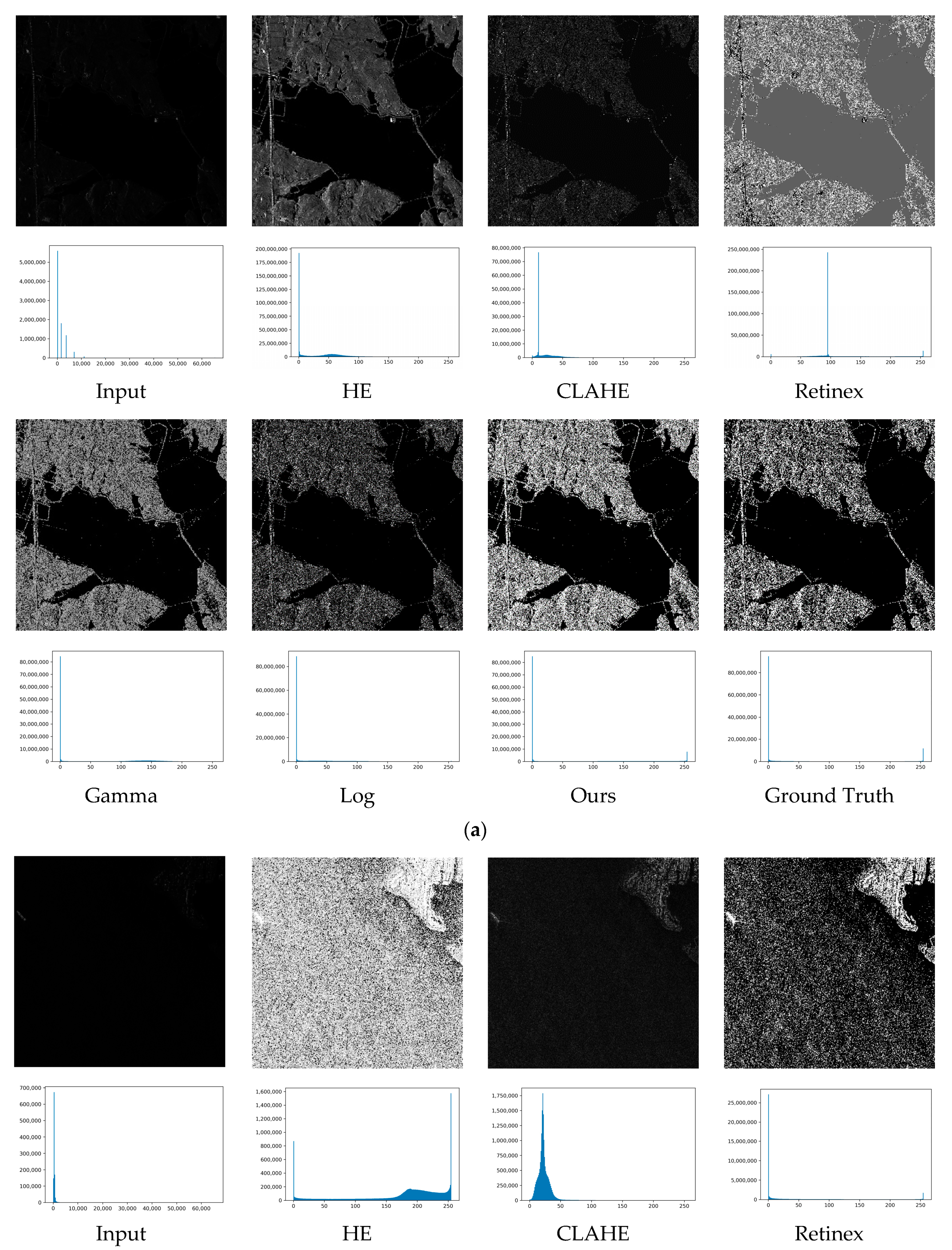
3.3. Results and Analysis

We compare the proposed method with traditional dynamic range compression algorithms: HE, CLAHE, Retinex, Gamma correction and logarithmic transformation, to verify the effectiveness of the proposed method. The results on synthetic and real SAR images from the visual and quantitative perspective are presented below.

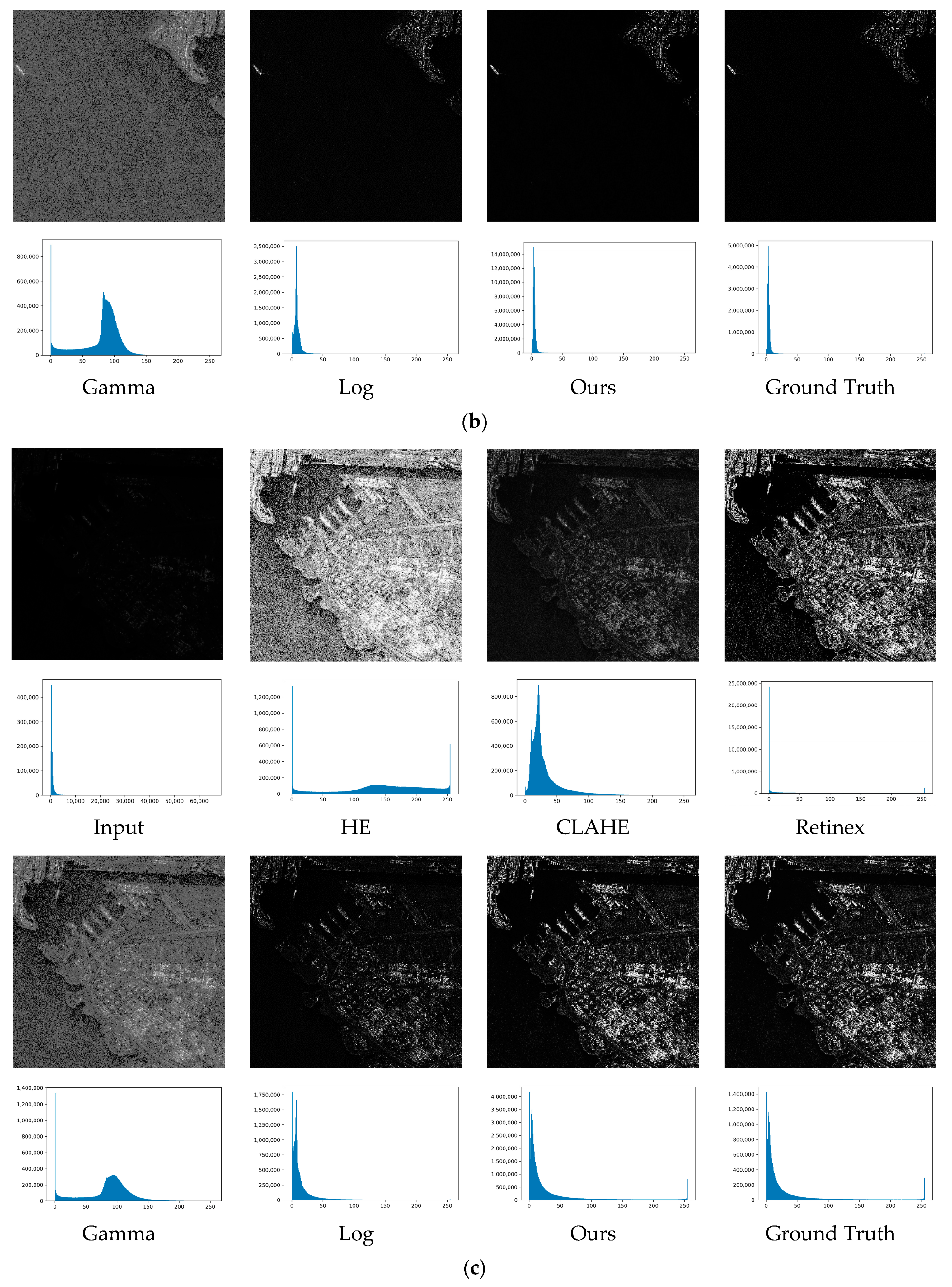
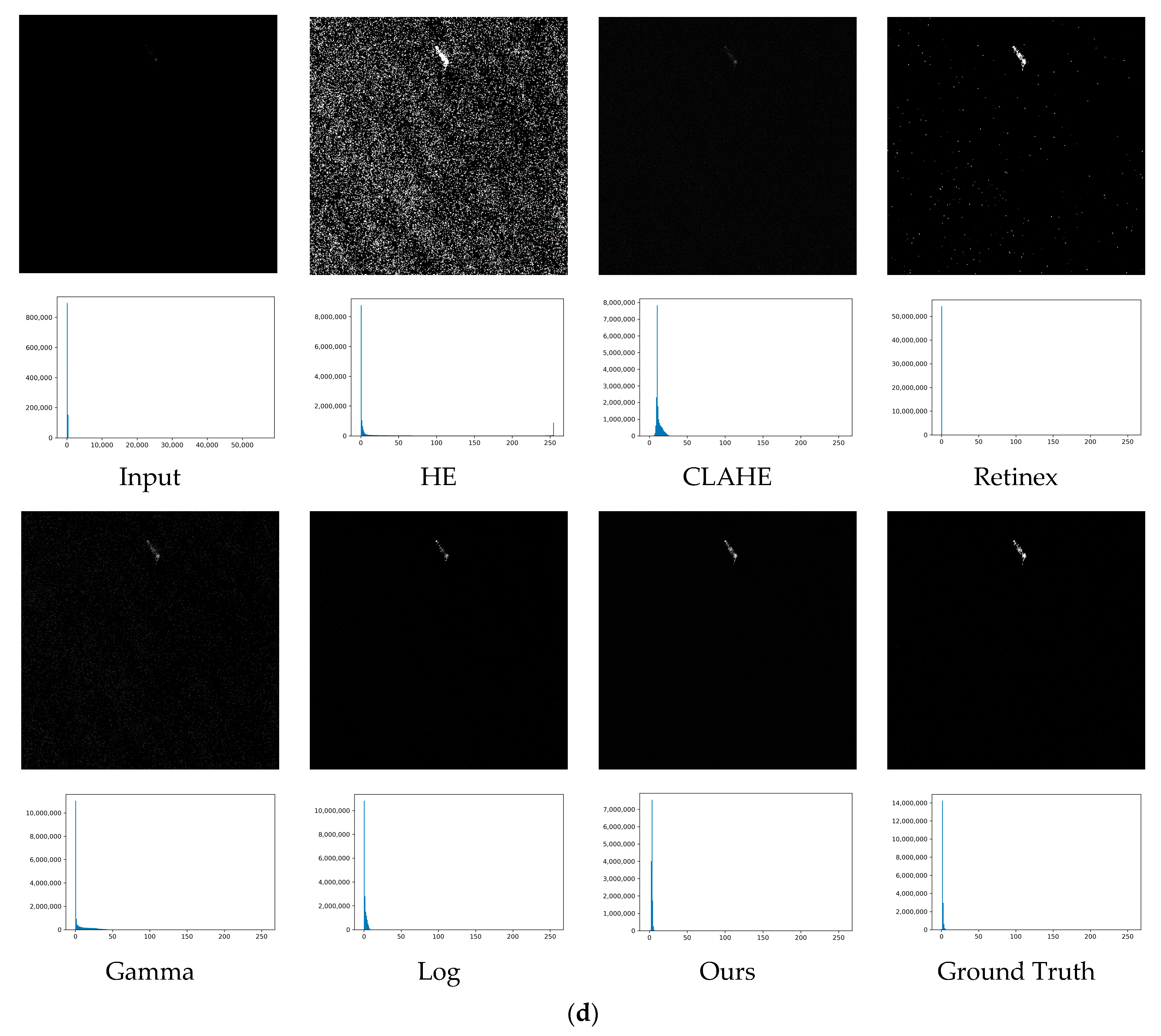
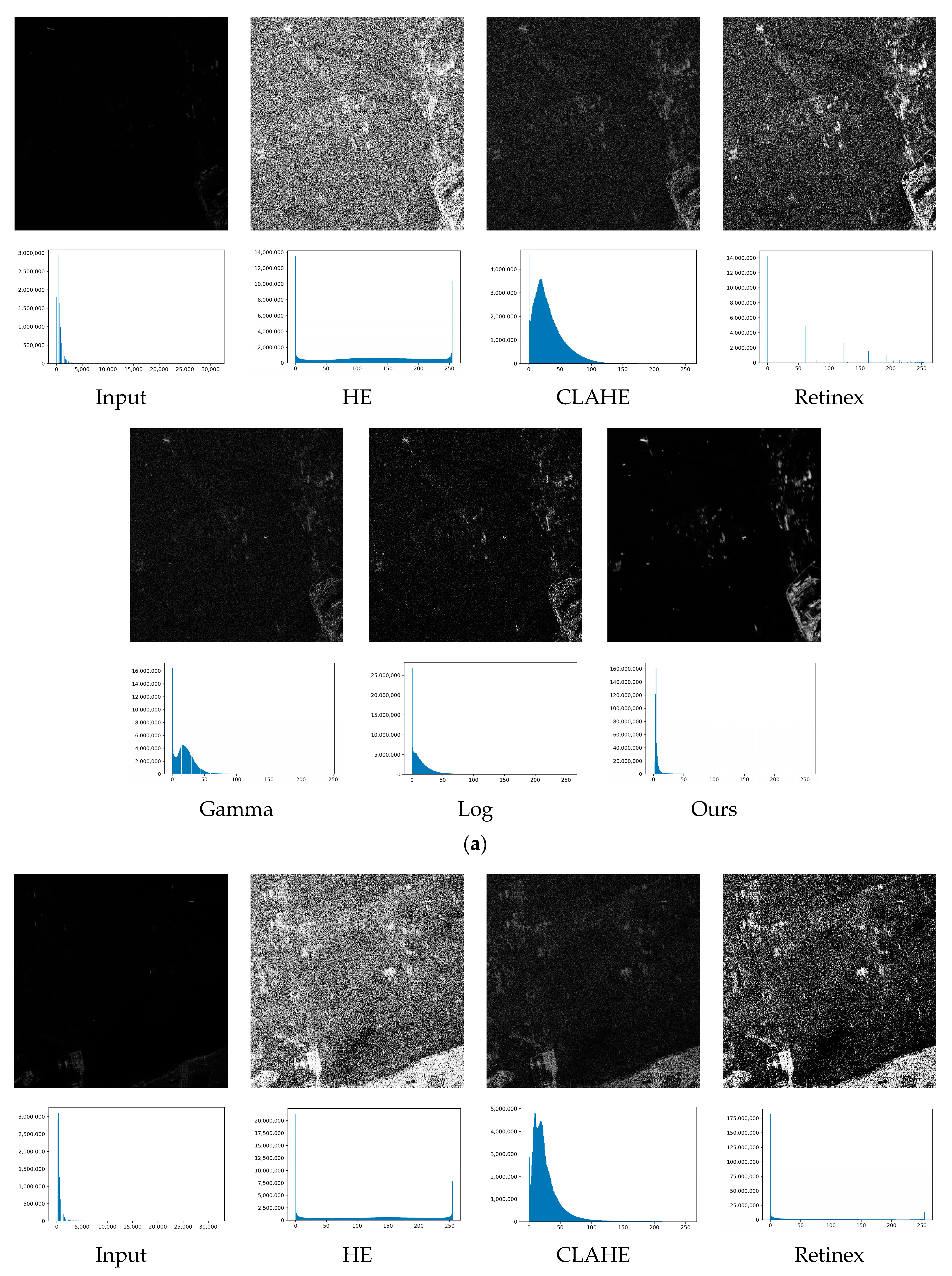
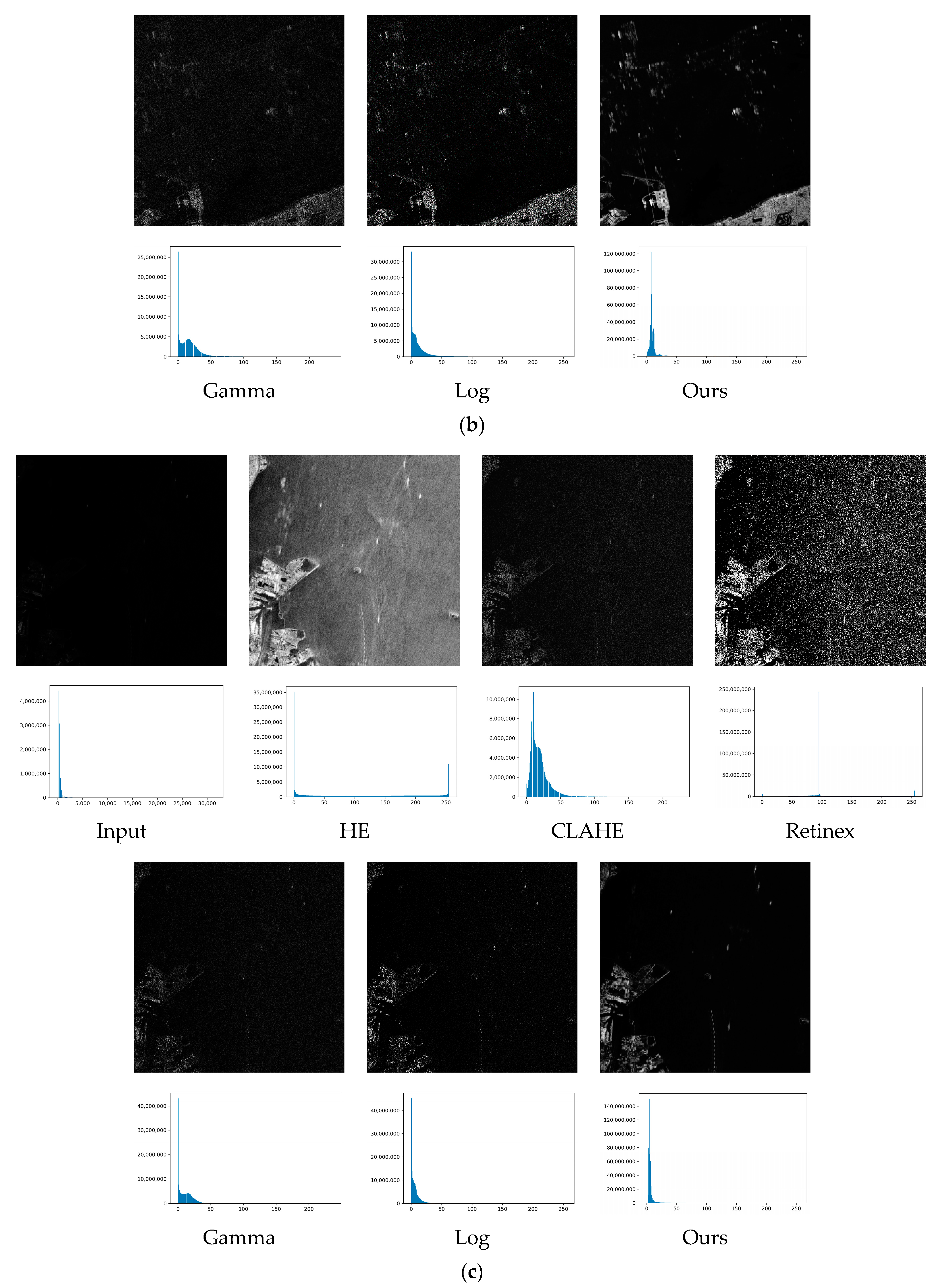
3.3.1. Experiments on Synthesized SAR Images

For the synthesized SAR images visualization experiments, a combination of visual and quantitative comparisons is used to analyze the effects of the different methods. Firstly, Figure 7 shows the visual results on synthesized SAR images.
It can be seen from the visual results that all methods can realize visualization to a certain extent. However, the traditional methods have defects on different fronts. The HE improves contrast significantly, while its result shows excessive enhancement. In other words, it leads to the loss of details and the distortion of structure, along with the amplification of noise. CLAHE prevents excessive enhancement by presetting a threshold value. But it has a poor performance in improving contrast. Retinex shows an acceptable tradeoff between proper contrast and detailed feature preservation. However, its results look distributed by noise in some scenes. In short, these adaptive algorithms have the above problems, and it is difficult to ensure the consistency of the visual effect. The Gamma correction and logarithmic transformation are not adaptive and depend on the selection of parameters. They even perform worse than the other methods. From the perspective of contrast enhancement, noise suppression, detail retention and adaptivity, the proposed algorithm is superior to the traditional algorithms. As shown in Figure 7, our method obtains better results compared to the traditional ones. This can be explained from two aspects: (1) Our method can notably improve contrast with better preserving details and suppressing noise; and (2) The method has high adaptivity and its results can maintain a consistency. Moreover, an important criterion for SAR image dynamic range compression is to preserve the intensity ranks in the output image. By observing the histogram of the input image, our method protects the ranks of the intensity levels in original SAR images compared with other methods. Besides, the histogram distribution of results achieved by our method is consistent with the ground truth. This also confirms the superiority of our method.
Except for the visual evaluation, quantitative evaluation is also necessary for comprehensive analysis of dynamic range compression performance. Table 1 lists the quantitative evaluation results with the best performance marked in bold. As we can see, our proposed method achieved the best results in terms of the PSNR and SSIM. This means that the results of our proposed method are closer to the ground truth, with better structure feature preservation and noise suppression.

3.3.2. Experiments on Real-world SAR Images

In order to further illustrate the practicability of the proposed method, we conduct experiments on real-world 16bit SAR images from AIR-SARShip-1.0 [42] dataset. The comparison results are shown in Figure 8.
The performance of these methods on real-world SAR images are similar to that on synthesized images. For CLAHE, Gamma correction, and logarithmic transformation, the cost of preserving detail is losing the contrast. And the latter two have poor adaptivity, which is not suitable for a practical application. In common with the results on synthesized images, a critical problem of HE and Retinex is that their results present an imbalance between contrast enhancement and noise suppression. It can disturb subsequent interpretations. By contrast, our method has good performance in solving the above problems. It can deal with original real-world SAR images in different scenes. Our method can still preserve the intensity ranks in the output image when dealing with real-world SAR images compared with other methods.
Due to ground truth not being able to be achieved as the reference, the PSNR and SSIM are no longer applicable for the real-world SAR dynamic range compression evaluation. Thus, we employ another two non-reference indexes, Entropy and EME. They can reflect the richness of information and the degree of contrast, respectively. Table 2 provides the quantitative comparison, with the best and second-best performance marked in bold and underlined.
As can be seen from Table 2, HE has a strong ability of improving contrast. However, it loses the detailed features of the excessive enhanced region. CLAHE surpasses other traditional methods in terms of information preservation according to its higher Entropy score. But it doesn’t have good performance in terms of improving contrast. Our method can always achieve the best or second-best numerical results. By combining the visual results, it showed good dynamic range compression ability in terms of contrast enhancement, noise suppression and detail preservation. It is practical in real scenes for SAR image visualization.

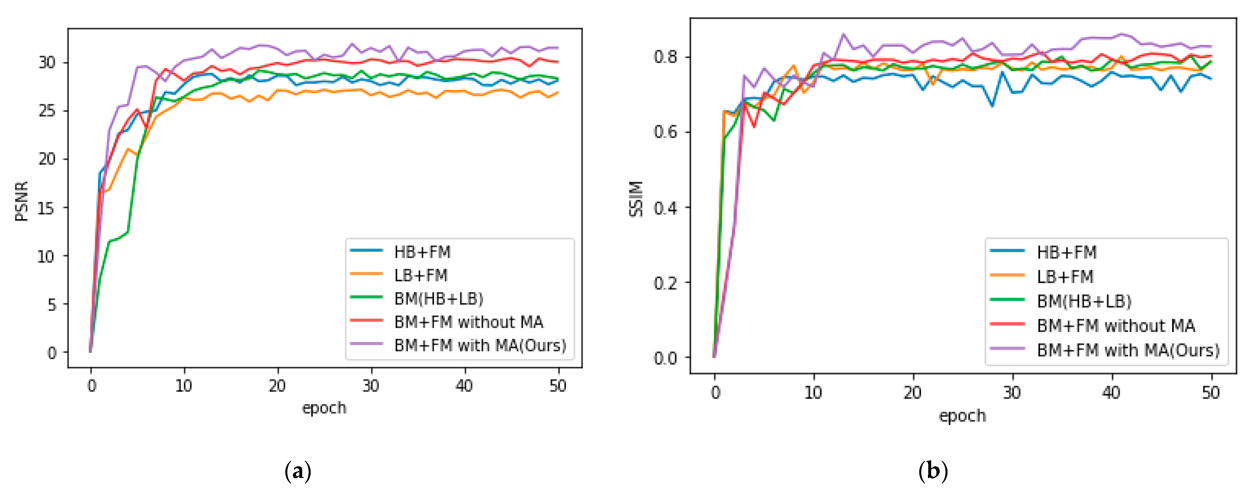
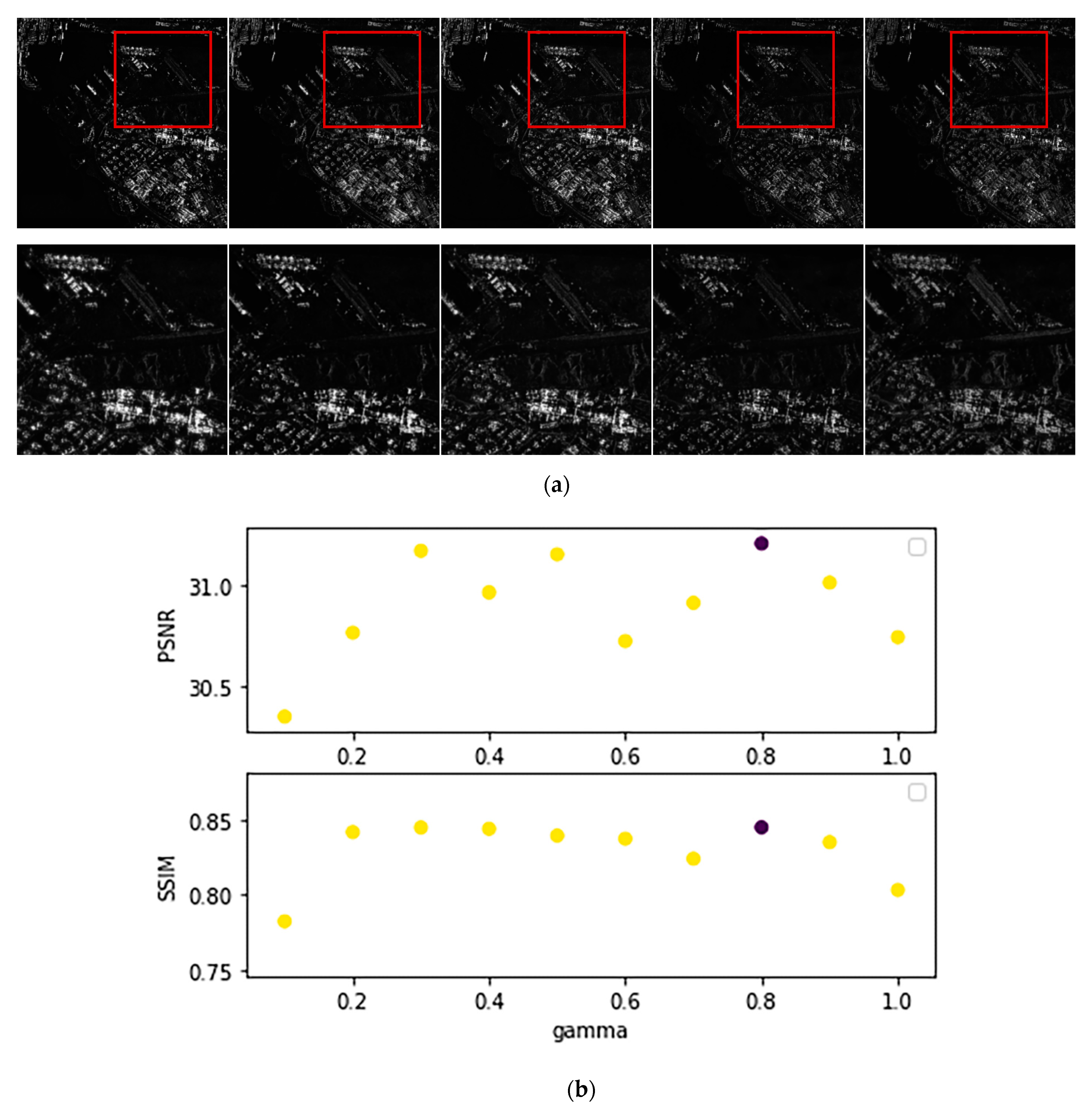
3.4. Ablation and Analysis

To further demonstrate the effectiveness of the proposed method, we conducted a series of ablation experiments on the framework, including high frequency feature branch (HB), low frequency feature branch (LB), bilateral feature enhancement module (BM), feature fusion module (FM), RRL unit, and MA. Figure 9, with SSIM and PSNR as evaluation metrics, shows the evaluation results of different network structures in each training stage on the verification set.
As shown in Figure 9, the decomposition-fusion framework proposed achieves a stable and good performance. By comparing the curves of HB + FM, LB + FM, BM, BM + FM without MA, we can ascertain the importance of the bilateral feature enhancement module and the feature fusion module. They supplement each other, and the step of decomposition and fusion is vital. High and low frequency features are both integral for fusion into a more precise description. The last two curves (BM + FM without MA, BM + FM with MA) present the effect of MA. After adopting the MA mechanism to bridge the corresponding layers of the encoder and decoder, the PSNR and SSIM scores rise sharply. It follows that the MA helps optimize the spatial feature representation. Furthermore, we list the numerical results of different network structures on the test set in Table 3 with the best performance in bold and the second-best ones underlined.
As seen in Table 3, the PSNR score employing the HB + FM structure is higher than employing LB + FM. It indicates that HB plays an important role in remapping high frequency features and suppressing noise. The other scores of the LB + FM structure are higher than that of HB + FM. It can be seen that LB has obvious advantages in remapping low frequency features and improving contrast.
To prove the effect of FM, we experimented with the increase and decrease of it. The improvement of various indicators shows that the FM can integrate bilateral features and optimize feature representation.
Though without MA, the decomposition-fusion framework has performed very well with regard to dynamic range compression. But after adding MA, the scores of PSNR, SSIM, Entropy and EME are all improving. MA helps select useful information for transmission and further suppresses noise.
In conclusion, the proposed method and modules have superior performance in SAR image dynamic range compression tasks. First, from the perspective of adaptivity, rapid visualization processing of SAR images is a problem of practical application. Our method can realize self-adaptive dynamic range compression compared with filter based and transfer function based methods. Second, it is better from the perspective of solving the existing problems. Detail loss and imbalance between contrast improvement and noise suppression are the main problems. Visual and quantitative experiments on synthesized and real-world SAR images show that the proposed method notably realizes visualization which exceeds several statistical methods. It has good adaptability and can improve SAR images’ contrast for interpretation.

4. Discussion

In this study, we designed a decomposition-fusion framework for SAR image dynamic range compression. This method can give an adaptive result for improving contrast, suppressing noise and preserving details. In order to make full use of high and low frequency features, a bilateral feature enhancement module is designed. It can establish the accurate feature description of SAR images by extracting and enhancing high and low frequency features of SAR images, respectively. To fuse the bilateral features effectively, we designed a feature fusion module for building adaptive and multi-scale context representation of SAR images. It can optimize the feature description to achieve a better result. In addition to these, the RRL unit and modified MA mechanism are proposed to optimize feature extraction and selection. Compared with traditional methods, the CNN-based method has the advantages of strong adaptability, and the performance of the decomposition-fusion framework proposed in this paper is far better than that of several dynamic range compression methods.
As mentioned earlier, the hybrid loss function takes the structure information and context information into consideration at the same time. It can boost the performance in our proposed framework. And the values of λ1 and λ2 are set to be 0.7 and 0.3. For the objective evaluation about L2 loss, MS-SSIM loss and hybrid loss function, we present their performance on four structures respectively, in terms of the average PSNR and SSIM scores. As shown in Figure 10a, the average PSNR and SSIM scores of hybrid loss function are larger than the others. Therefore, the hybrid loss function can improve the performance of the network generally.
In addition, to explain the reason for selecting the λ1 and λ2 values, we provide a set of comparative experiments. λ1 is set from 0 to 1, with interval of 0.1, and λ2 equals to 1 − λ1. As shown in Figure 10b, the average PSNR and SSIM scores of λ1 = 0.7 are larger than those of other values. This was because when λ1 = 0.7 and λ2 = 0.3, the framework can concentrate on structure information and context information properly. Hence, 0.7 and 0.3 are the superior value of λ1 and λ2, and the hybrid loss function can effectively boost the performance of our proposed framework for SAR image dynamic range compression.
We also present the reason for setting the gamma value to 0.8. The Gamma correction fine-tunes the weight graph to avoid excessive enhancement and information loss. For the visual results under different gamma values, only 1, 0.9, 0.8, 0.7, 0.6 are compared in Figure 11a. Because when the gamma value is too small, the contrast of generated images is too low, so we omit the others’ visual results. As we can see in Figure 11a, the contrast increases as the gamma value improves. However, the information from the low pixel values region is lost. To achieve balance between the high contrast and the information preservation, we set the gamma value to be 0.8 according to the visual results. On the other hand, the average PSNR and SSIM scores of gamma value = 0.8 are larger than those of other values. Thus, the chosen value can improve the performance of our proposed method.

5. Conclusions

In this paper, a decomposition-fusion framework for SAR image dynamic range compression is proposed. First, a bilateral feature enhancement module is designed to extract and enhance high and low frequency features. It can realize noise suppression and contrast improvement. Then, a feature fusion module is designed for fusing bilateral features. It can integrate bilateral features and optimize feature reconstruction. We also propose an RRL unit to improve the ability of the extracting features, and employ a modified MA mechanism to further enhance this useful feature. In addition, the proposed method is compared with traditional SAR image dynamic range compression methods from qualitative and quantitative perspectives, and the experimental results show that the proposed method is effective and practical.
Because of the lack of paired data sets, unsupervised deep learning will be studied in future work for SAR image visualization, and a better network will be designed by combining the characteristics of SAR images.

Author Contributions

Conceptualization, H.S.; methodology, H.S. and Q.S.; validation, H.S. and Q.S.; writing—original draft preparation, Q.S.; writing—review and editing, H.S. and Q.S.; supervision, Y.W. and B.Y.; funding acquisition, L.C. All authors have read and agreed to the published version of the manuscript.

Funding

This work was supported in National Natural Science Foundation of China No.62101041, the Chang Jiang Scholars Program under Grant T2012122 and the Hundred Leading Talent Project of Beijing Science and Technology under Grant Z141101001514005.

Data Availability Statement

Sentinel-1 data is available at https://scihub.copernicus.eu/ (accessed on 29 November 2021). AIR-SARShip-1.0 data is available at https://radars.ac.cn/web/data/getData?dataType=SARDataset (accessed on 4 June 2021).

Acknowledgments

The authors would like to thank the European Space Agency (ESA) for providing free Sentinel-1 data. The authors would also like to thank the anonymous reviewers for their very competent comments and helpful suggestions.

Conflicts of Interest

The authors declare that they have no conflicts of interests.

Abbreviation

AbbreviationDefinition
SARSynthetic Aperture Radar
HDRHigh Dynamic Range
LDRLow Dynamic Range
CAMChannel Attention Module
RRLResidual Recursive Learning Unit
MAMulti-scale Attention Module
HBHigh frequency feature Branch
LBLow frequency feature Branch
BMBilateral feature enhancement Module
FMFeature fusion Module
PBPreprocessing Block
EBEncoder Block
MBMiddle Block
DBDecoder Block
OBOutput Block
PSNRPeak Signal-to-Noise Ratio
SSIMStructural Similarity Index
HEHistogram Equalization
CLAHEContrast Adaptive Limitation Histogram Equalization

References

  1. Moreira, A.; Prats-Iraola, P.; Younis, M.; Krieger, G.; Hajnsek, I.; Papathanassiou, K.P. A tutorial on synthetic aperture radar. IEEE Geosci. Remote Sens. Mag. 2013, 1, 6–43. [Google Scholar] [CrossRef] [Green Version]
  2. Pizer, S.M.; Amburn, E.P.; Austin, J.D.; Cromartie, R.; Geselowitz, A.; Greer, T.; ter Haar Romeny, B.; Zimmerman, J.B.; Zuiderveld, K. Adaptive histogram equalization and its variations. Comput. Vis. Graph. Image Process. 1987, 39, 355–368. [Google Scholar] [CrossRef]
  3. Stark, J.A. Adaptive Image Contrast Enhancement Using Generalizations of Histogram Equalization. IEEE Trans. Image Process. 2000, 9, 889–896. [Google Scholar] [CrossRef] [PubMed] [Green Version]
  4. Reza, A.M. Realization of the contrast limited adaptive histogram equalization (CLAHE) for real-time image enhancement. J. VLSI Signal Process. Syst. Signal Image Video Technol. 2004, 38, 35–44. [Google Scholar] [CrossRef]
  5. Land, E.H.; McCann, J.J. Lightness and retinex theory. J. Opt. Soc. Am. 1971, 61, 1–11. [Google Scholar] [CrossRef]
  6. Jobson, D.; Rahman, Z.; Woodell, G. Properties and performance of a center/surround retinex. IEEE Trans. Image Process. 1997, 6, 451–462. [Google Scholar] [CrossRef]
  7. Rahman, Z.; Jobson, D.J.; Woodell, G. Multiscale retinex for color image enhancement. In Proceedings of the 3rd IEEE International Conference on Image Processing, Lausanne, Switzerland, 19 September 1996. [Google Scholar]
  8. Farid, H. Blind inverse gamma correction. IEEE Trans. Image Process. 2001, 10, 1428–1433. [Google Scholar] [CrossRef]
  9. Drago, F.; Myszkowski, K.; Annen, T.; Chiba, N. Adaptive Logarithmic Mapping for Displaying High Contrast Scenes. In Computer Graphics Forum; Blackwell Publishing, Inc.: Oxford, UK, 2003; Volume 22. [Google Scholar]
  10. Li, Z.; Liu, J.; Huang, J. Dynamic range compression and pseudo-color presentation based on Retinex for SAR images. In Proceedings of the 2008 International Conference on Computer Science and Software Engineering, Wuhan, China, 12–14 December 2008; Volume 6, pp. 257–260. [Google Scholar]
  11. Hisanaga, S.; Wakimoto, K.; Okamura, K. Tone mapping and blending method to improve SAR image visibility. IAENG Int. J. Comput. Sci. 2011, 38, 289–294. [Google Scholar]
  12. Hisanaga, S.; Wakimoto, K.; Okamura, K. Compression method for high dynamic range intensity to improve sar image visibility. In Proceedings of the International MultiConference of Engineers and Computer Scientists, Hong Kong, 16–18 March 2011; Volume 1. [Google Scholar]
  13. Upadhyay, A.; Mahapatra, S. Adaptive enhancement of compressed SAR images. Signal Image Video Process. 2016, 10, 1335–1342. [Google Scholar] [CrossRef]
  14. Lai, R.; Guan, J.; Yang, Y.; Xiong, A. Spatiotemporal adaptive nonuniformity correction based on BTV regularization. IEEE Access 2018, 7, 753–762. [Google Scholar] [CrossRef]
  15. Tirandaz, Z.; Akbarizadeh, G. A two-phase algorithm based on kurtosis curvelet energy and unsupervised spectral regression for segmentation of SAR images. IEEE J. Sel. Top. Appl. Earth Obs. Remote Sens. 2015, 9, 1244–1264. [Google Scholar] [CrossRef]
  16. Zhao, Y.; Wang, S.; Jiao, L.; Li, K. SAR image despeckling based on sparse representation. In MIPPR 2007: Multispectral Image Processing. International Society for Optics and Photonics. Proceedings of the International Symposium on Multispectral Image Processing and Pattern Recognition, Wuhan, China, 15–17 November 2007; SPIE: Bellingham, WA, USA, 2007; Volume 6787, p. 67872I. [Google Scholar]
  17. Dabov, K.; Foi, A.; Katkovnik, V.; Egiazarian, K. Image denoising with block-matching and 3D filtering. In Image Processing: Algorithms and Systems, Neural Networks, and Machine Learning. International Society for Optics and Photonics. Proceedings of the Electronic Imaging 2006, San Jose, CA, USA, 16–19 January 2006; SPIE: Bellingham, WA, USA, 2006; Volume 6064, p. 606414. [Google Scholar]
  18. Bioucas-Dias, J.M.; Figueiredo, M.A.T. Multiplicative noise removal using variable splitting and constrained optimization. IEEE Trans. Image Process. 2010, 19, 1720–1730. [Google Scholar] [CrossRef] [PubMed] [Green Version]
  19. Chierchia, G.; Cozzolino, D.; Poggi, G.; Verdoliva, L. SAR image despeckling through convolutional neural networks. In Proceedings of the 2017 IEEE International Geoscience and Remote Sensing Symposium (IGARSS), Fort Worth, TX, USA, 23–28 July 2017; pp. 5438–5441. [Google Scholar]
  20. Zhang, Q.; Yuan, Q.; Li, J.; Yang, Z.; Ma, X. Learning a dilated residual network for SAR image despeckling. Remote Sens. 2018, 10, 196. [Google Scholar] [CrossRef] [Green Version]
  21. Li, J.; Li, Y.; Xiao, Y.; Bai, Y. Hdranet: Hybrid dilated residual attention network for SAR image despeckling. Remote Sens. 2019, 11, 2921. [Google Scholar] [CrossRef] [Green Version]
  22. Zhang, K.; Zuo, W.; Chen, Y.; Meng, D.; Zhang, L. Beyond a gaussian denoiser: Residual learning of deep CNN for image denoising. IEEE Trans. Image Process. 2017, 26, 3142–3155. [Google Scholar] [CrossRef] [PubMed] [Green Version]
  23. Ronneberger, O.; Fischer, P.; Brox, T. U-net: Convolutional networks for biomedical image segmentation. In Proceedings of the International Conference on Medical Image Computing and Computer-Assisted Intervention, Munich, Germany, 5–9 October 2015. [Google Scholar]
  24. Gharbi, M.; Chen, J.; Barron, J.T.; Hasinoff, S.W.; Durand, F. Deep bilateral learning for real-time image enhancement. ACM Trans. Graph. 2017, 36, 1–12. [Google Scholar] [CrossRef]
  25. Ignatov, A.; Kobyshev, N.; Timofte, R.; Vanhoey, K. DSLR-quality photos on mobile devices with deep convolutional networks. In Proceedings of the IEEE International Conference on Computer Vision, Venice, Italy, 22–29 October 2017. [Google Scholar]
  26. Goodfellow, I.; Pouget-Abadie, J.; Mirza, M.; Xu, B.; Warde-Farley, D.; Ozair, S.; Courville, A.; Bengio, Y. Generative adversarial nets. In Proceedings of the Advances in Neural Information Processing Systems 27 (NIPS 2014), Montreal, QC, Canada, 8–13 December 2014; Volume 27.
  27. Caballero, J.; Ledig, C.; Aitken, A.; Acosta, A.; Totz, J.; Wang, Z.; Shi, W. Real-time video super-resolution with spatio-temporal networks and motion compensation. In Proceedings of the IEEE Conference on Computer Vision and Pattern Recognition, Honolulu, HI, USA, 21–26 July 2017; pp. 4778–4787. [Google Scholar]
  28. Ledig, C.; Theis, L.; Huszár, F.; Caballero, J.; Cunningham, A.; Acosta, A.; Aitken, A.; Tejani, A.; Totz, J.; Wang, Z.; et al. Photo-realistic single image super-resolution using a generative adversarial network. In Proceedings of the IEEE Conference on Computer Vision and Pattern Recognition, Honolulu, HI, USA, 21–26 July 2017; pp. 4681–4690. [Google Scholar]
  29. Remez, T.; Litany, O.; Giryes, R.; Bronstein, A.M. Deep class-aware image denoising. In Proceedings of the 2017 International Conference on Sampling Theory and Applications (SampTA), Tallinn, Estonia, 3–7 July 2017; pp. 138–142. [Google Scholar]
  30. Isola, P.; Zhu, J.Y.; Zhou, T.; Efros, A.A. Image-to-image translation with conditional adversarial networks. In Proceedings of the IEEE Conference on Computer Vision and Pattern Recognition, Honolulu, HI, USA, 21–26 July 2017; pp. 1125–1134. [Google Scholar]
  31. Zhu, J.Y.; Park, T.; Isola, P.; Efros, A.A. Unpaired image-to-image translation using cycle-consistent adversarial networks. In Proceedings of the IEEE International Conference on Computer Vision, Honolulu, HI, USA, 21–26 July 2017; pp. 2223–2232. [Google Scholar]
  32. Yan, Z.; Zhang, H.; Wang, B.; Paris, S.; Yu, Y. Automatic photo adjustment using deep neural networks. ACM Trans. Graph. 2016, 35, 1–15. [Google Scholar] [CrossRef]
  33. Tao, L.; Zhu, C.; Xiang, G.; Li, Y.; Jia, H.; Xie, X. LLCNN: A convolutional neural network for low-light image enhancement. In Proceedings of the 2017 IEEE Visual Communications and Image Processing (VCIP), St. Petersburg, FL, USA, 10–13 December 2017; pp. 1–4. [Google Scholar]
  34. Lore, K.G.; Akintayo, A.; Sarkar, S. LLNet: A deep autoencoder approach to natural low-light image enhancement. Pattern Recognit. 2017, 61, 650–662. [Google Scholar] [CrossRef] [Green Version]
  35. He, K.; Zhang, X.; Ren, S.; Sun, J. Delving deep into rectifiers: Surpassing human-level performance on imagenet classification. In Proceedings of the IEEE International Conference on Computer Vision, Santiago, Chile, 11–18 December 2015; pp. 1026–1034. [Google Scholar]
  36. Yu, F.; Koltun, V.; Funkhouser, T. Dilated residual networks. In Proceedings of the IEEE Conference on Computer Vision and Pattern Recognition, Honolulu, HI, USA, 21–26 July 2017; pp. 472–480. [Google Scholar]
  37. Kingma, D.; Ba, J. Adam: A Method for Stochastic Optimization. arXiv 2014, arXiv:1412.6980. [Google Scholar]
  38. Lattari, F.; Gonzalez Leon, B.; Asaro, F.; Rucci, A.; Prati, C.; Matteucci, M. Deep learning for SAR image despeckling. Remote Sens. 2019, 11, 1532. [Google Scholar] [CrossRef] [Green Version]
  39. Wang, Z.; Bovik, A.C.; Sheikh, H.R.; Simoncelli, E.P. Image quality assessment: From error visibility to structural similarity. IEEE Trans. Image Process. 2004, 13, 600–612. [Google Scholar] [CrossRef] [PubMed] [Green Version]
  40. Watson, A.B.; Borthwick, R.; Taylor, M. Image quality and entropy masking. In Human Vision and Electronic Imaging II. International Society for Optics and Photonics. Proceedings of the Electronic Imaging’97, San Jose, CA, USA, 8–14 February 1997; SPIE: Bellingham, WA, USA, 1997; Volume 3016, pp. 2–12. [Google Scholar]
  41. Sundaram, M.; Ramar, K.; Arumugam, N.; Prabin, G. Histogram modified local contrast enhancement for mammogram images. Appl. Soft Comput. 2011, 11, 5809–5816. [Google Scholar] [CrossRef]
  42. Xian, S.; Zhirui, W.; Yuanrui, S.; Wenhui, D.; Yue, Z.; Kun, F. AIR-SARShip–1.0: High resolution SAR ship detection dataset. Radars 2019, 8, 852–862. [Google Scholar]
Figure 1. Overview of the proposed decomposition-fusion framework.
Remotesensing 14 02338 g001
Figure 2. Structure of proposed bilateral feature enhancement module. (a) Details of bilateral feature enhancement module which consists of high frequency feature branch and low frequency feature branch. (b) Details of ResBlock. (c) Details of DilationBlock.
Remotesensing 14 02338 g002
Figure 3. Structure of proposed feature fusion module.
Remotesensing 14 02338 g003
Figure 4. The detailed structure of an RRL Unit.
Remotesensing 14 02338 g004
Figure 5. The detailed structure of multi-scale attention mechanism.
Remotesensing 14 02338 g005
Figure 6. Examples of synthesized SAR image slices. The histogram exhibits the pixel distribution in the image. (a) Original SAR images to be visualized. (b) Corresponding ground truth.
Remotesensing 14 02338 g006
Figure 7. Visual results on synthesized images. The histogram exhibits the pixel distribution in the image. (ad) Comparison of different single images.
Remotesensing 14 02338 g007aRemotesensing 14 02338 g007bRemotesensing 14 02338 g007c
Figure 8. Visual results on real SAR images. The histogram exhibits the pixel distribution in the image. (ac) Comparison of different single images.
Remotesensing 14 02338 g008aRemotesensing 14 02338 g008b
Figure 9. Ablation experiment results on test set. (a) PSNR scores of different structures. (b) SSIM scores of different structures.
Remotesensing 14 02338 g009
Figure 10. Evaluation of hybrid loss function. (a) Performance of L2 loss, MS-SSIM loss and hybrid loss function on different structures. (b) Performance of hybrid loss function under different λ1 and λ2 values on proposed framework.
Remotesensing 14 02338 g010
Figure 11. Evaluation of different gamma values. (a) Visual results under gamma values of 1, 0.9, 0.8, 0.7, 0.6. (b)Numerical results under gamma values from 0.1 to 1, with interval of 0.1.
Remotesensing 14 02338 g011
Table 1. Numerical results on synthesized images. The highest scores are marked in bold.
Image 1Image 2Image 3Image 4
PSNRSSIMPSNRSSIMPSNRSSIMPSNRSSIM
HE6.5720.5277.3970.4937.3240.4906.7210.587
CLAHE25.2930.58425.4310.57225.4450.57125.2400.589
Retinex20.6630.75320.6750.78120.1420.77420.1460.745
Gamma21.1930.53821.6900.57421.0310.57621.8320.508
Log23.1620.53123.5320.58523.0430.58123.8490.517
Proposed31.3080.84531.7740.89031.8660.89431.2670.838
Table 2. Numerical results on real SAR images. The highest and second-highest scores are marked in bold and underlined respectively.
Image 1Image 2Image 3
EntropyEMEEntropyEMEEntropyEME
HE6.1958950.9221715.4936930.9207503.4069620.921220
CLAHE8.5332010.7919218.1032210.7784174.7345640.741041
Retinex5.1726130.8583654.1646170.8295911.3219040.798544
Gamma3.7073920.74733.0594690.74210.8743830.7116
Log3.6958610.83013.0348590.81880.8705040.8031
Proposed7.7790420.92185510.723570.9204898.0816260.920724
Table 3. Numerical analysis of different structures. The highest and second-highest scores are marked in bold and underlined respectively.
PSNRSSIMEntropyEME
HB + FM28.5540.7572.9380.644
LB + FM27.0580.7994.0680.843
BM (HB + LB)28.9830.8084.4170.828
BM + FM without MA30.3410.8105.0810.887
BM + FM with MA(Ours)31.8170.8485.4970.899
Publisher’s Note: MDPI stays neutral with regard to jurisdictional claims in published maps and institutional affiliations.

