1. Introduction
Being able to remotely identify individual species or taxa of invasive aquatic plants and map their extent would be useful to their management. Identifying a vegetation class or dominant vegetation group may also be useful. The management of submerged aquatic vegetation (SAV) is common because of verified and perceived negative impacts. For example, invasive plants that grow as SAV can have significant impacts on aquatic systems, such as reduced dissolved oxygen levels, a greater presence of non-native fishes, reduced plant species richness, reduced forage value for waterfowl and macroinvertebrates, reduced human use of littoral zones, and a negative influence on zooplankton abundance [
1,
2,
3,
4]. However, in some cases, total species diversity may not be lower in invaded aquatic plant communities [
2], the overall productivity can be the same [
5], and invasive aquatic plants may provide their own level of beneficial ecosystem services [
6]. Therefore, understanding the identity and distribution of species of SAV in lake littoral zones is an important challenge that could be addressed using remote sensing. Addressing this challenge will depend on our ability to remotely identify SAV in the optically complex waters characteristic of lake littoral zones.
This paper focuses on the deployment of multispectral cameras from an uncrewed aerial system (UAS or “drone”) platform to enable rapid, timely imaging of
Myriophyllum spicatum (Eurasian watermilfoil, or EWM) to identify its extent in littoral zones. EWM has been shown to reduce native species abundance [
7,
8] and suppress native plants [
9], lower lakeshore property values through interference with boating recreation [
10], impact swimming recreation [
9], and it can increase phosphorus (P) loads during decomposing after herbicide application [
11]. EWM was known to be present in the Laurentian Great Lakes by the early 1950s [
12], and it grows most abundantly in one to four meters of water [
13].
The capabilities of UAS have been increasing in recent years, gaining the attention of ecologists as useful tools for meeting environmental data needs, including the mapping of SAV and other features of interest [
14,
15,
16]. Recent work has shown the utility of UAS imagery for identifying the extent of invasive wetland plants [
17] and further investigated floating and aquatic plant mapping [
18]. The intermediate scale between satellite imagery and field observations that UAS data can produce is able to provide ecologically relevant results of aquatic plant identification, extent, and change [
19]. A UAS can also be deployed during optimal weather conditions (low winds, more sunlight, optimal sun angles) and collect high-resolution imagery that may help with the differentiation of species of interest, from animals to aquatic plants [
19,
20,
21]. The highest resolution multispectral satellite imagery bands available at the start of this study were 1.84 m pixel size, and we anticipated that the higher-resolution capabilities of UAS multispectral sensing would provide data more useful for the identification of EWM.
The amount of light penetration into a lake’s water column is a controlling factor for the species that exist in particular areas and helps to define the littoral zone where SAV grows. Some invasive species of SAV have an advantageous ability to grow in littoral zones with lower light penetration than many native species [
22]. Therefore, being able to reliably identify SAV to species or taxon in areas with higher extinction coefficients (lower water clarity) could help with understanding the extent of invasive SAV taxa. The extinction coefficient of light in water is impacted by three main color-producing agents (CPAs): chlorophyll (CHL), suspended minerals (SM), and the colored dissolved organic matter (CDOM) component of dissolved organic carbon (DOC) [
23]. Because of these CPAs, inland waters can be highly optically complex [
24], and CPA concentrations can change significantly over relatively short time intervals [
25]. We expect that SAV will be harder to identify in areas affected by one or more CPAs, reducing light transmission, than in areas that have higher water clarity. For example, in areas with a local tributary contribution of CDOM, it may be more difficult to identify where SAV is located than in areas without sources contributing this CPA component.
Potentially important to EWM identification is how well mixed it is with other SAV species. The presence vs. absence of EWM, such as EWM vs. open water, is likely to be relatively simple to differentiate. However, when EWM is mixed in with several other species that may appear similar to the naked eye in visible light, it is likely to be more difficult to separate using readily available natural color (red/green/blue or RGB) cameras or those with a relatively small number of multispectral bands. In our previous research [
26], we demonstrated that spectral profiles of submerged aquatic vegetation (SAV) can be used to identify EWM when using certain indices and bands. A modified Normalized Difference Vegetation Index (mNDVI) was significantly different for EWM vs. other submerged aquatic vegetation, providing a potential means of identifying EWM with high-resolution remote sensing data. The mNDVI replaced the use of infrared light, normally around 850 nm, with a shorter wavelength of 720 nm that penetrates further into the water. This was tested for EWM detection in depths up to 2.5 m, the maximum depth recorded for EWM that was later interpreted into classification results. Averaging spectral data to sixty-five 10 nm wide bands, similar to available hyperspectral systems, provided an ability to differentiate EWM from other species of SAV, whereas using only six to eight bands only worked occasionally. At particular sites on certain dates, individual taxa could be identified using only the six to eight multispectral bands that corresponded to the bands of the project’s main multispectral sensor. However, for a majority of spectral comparisons, this number of bands was not sufficient to differentiate EWM from other taxa.
We have applied the finding that the mNDVI could possibly differentiate EWM from other SAV species [
26] to identify the extent of EWM in a part of the Laurentian Great Lakes. We focused on understanding the accuracy of our EWM mapping using the mNDVI derived from multispectral UAS imagery. The paper includes an analysis of whether accounting for water clarity using two different classification parameters can improve the mapping of SAV, as described below. Moving from analyzing spectral profiles to imaging EWM and other SAV in the field is the next step in a process for using remote sensing as a practical tool in invasive SAV management.
2. Methods
2.1. Collection Sites and UAS-Based Sensors Deployed for the Project
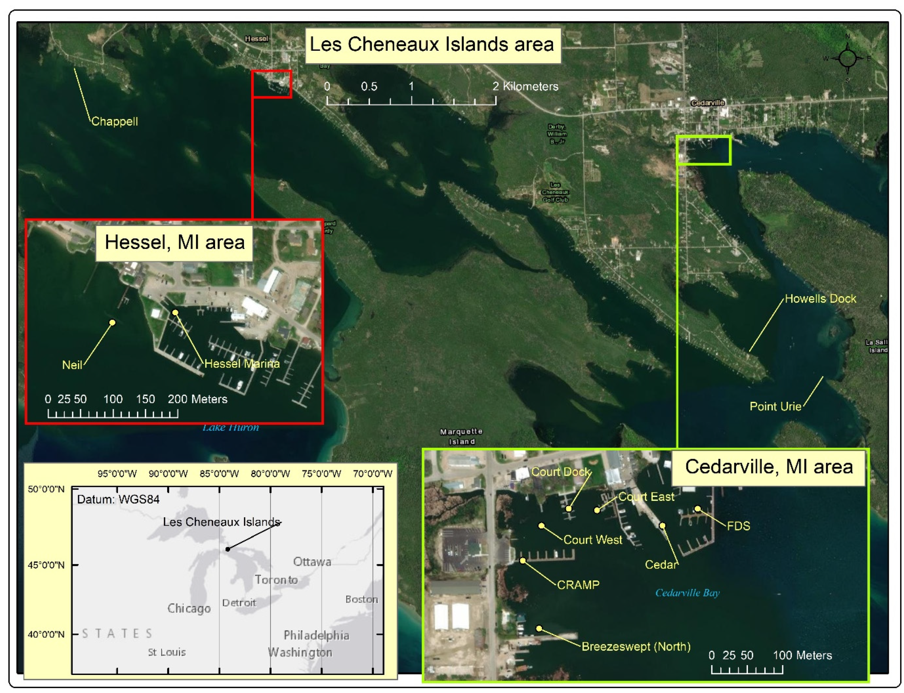
We collected data on CPAs and vegetation characteristics at several sites in the Les Cheneaux Islands area of northwest Lake Huron (MI, USA) (
Figure 1), our study site from [
26] that has previously been reported as having significant presence of EWM [
27].
We sampled 11 sites in the Les Cheneaux Islands over six trips in 2016–2018; the sampling months and the sensor we were able to deploy on each sampling occasion are shown in
Table 1. Three RGB-only camera systems were deployed via UAS, primarily to provide basemaps of the sites; these cameras were a Nikon D810 36mp camera flown onboard a Bergen hexacopter, the 12mp camera of a Phantom 3 Advanced (3A) UAS, and the 12mp camera of a Mavic Pro UAS. The U.S.-made Bergen hexacopter is a larger system that can carry payloads up to 5 kg for up to 15 min of flight. The Phantom 3 Advanced and Mavic Pro UAS are made by DJI and are designed to easily obtain RGB aerial photos but are not intended to carry additional payloads.
The six-band Tetracam Micro-MCA (Tetracam Inc., Chatsworth, CA, USA) described in [
26] was deployed onboard the Bergen hexacopter to evaluate whether its multispectral capabilities could help distinguish EWM from other aquatic cover types. Also described in [
26] is the VISNIR system which used a 16mp RGB Canon camera and a near-infrared-sensitive Canon camera. This was deployed on occasion using the Bergen hexacopter as a less costly potential alternative to the Tetracam for EWM identification purposes. The Tetracam sensor was not always available as it was a rental unit used starting in the second data collection of August 2016. When it was not available, we usually deployed the VISNIR system, such as in June 2017. We anticipated that the VISNIR near-infrared image band would not penetrate as far in the water with its longer wavelength than the red-edge capabilities of the Tetracam. Time limitations in the field, or issues with equipment operating properly, sometimes prevented operation of either system. Optical (RGB) imagery was collected at every site on every visit (
Table 1).
The Bergen hexacopter was used to deploy the Nikon RGB, Tetracam multispectral, or VISNIR system one at a time. The RGB camera systems used in this project had on-board global positioning systems (GPS) to provide positional data for every RGB photo. The Phantom 3A Advanced and Mavic 2 Pro were used to collect RGB imagery over larger areas. The RGB image sets for each site were developed into georeferenced orthophotos using Agisoft Metashape with approximately three-meter positional accuracy. Marker buoy locations recorded with a Trimble GeoExplorer 6000 with approximately 10 to 50cm positional accuracy (after differential correction) provided additional information for georeferencing. The RGB basemaps were also used to provide georeferencing of the Tetracam images, as that sensor did not have a built-in global navigation satellite system (GNSS) receiver for recording position. For multispectral imagery in 2016, we mostly flew at heights of 10–15 m, which produced images covering approximately a 3 × 3 m area with approximately 5 cm water surface resolution for the Tetracam, whereas we flew at heights of 25–30 m to cover larger areas in each image for 2017 and 2018 with approximately 8 to 10 cm resolution. Each sensor usually took one flight ranging from 10 to 20 min to complete, although larger RGB basemap flights for areas with multiple sites, such as the “Court sites”, could take up to three or four flights. RGB imagery was approximately 1 cm resolution with the Nikon D810 camera and approximately 2 cm with the P3A, Mavid, and VISNIR systems. After our first year of data collection, we decided that being able to cover larger areas was worth the trade-off of producing lower-resolution imagery when flying higher.
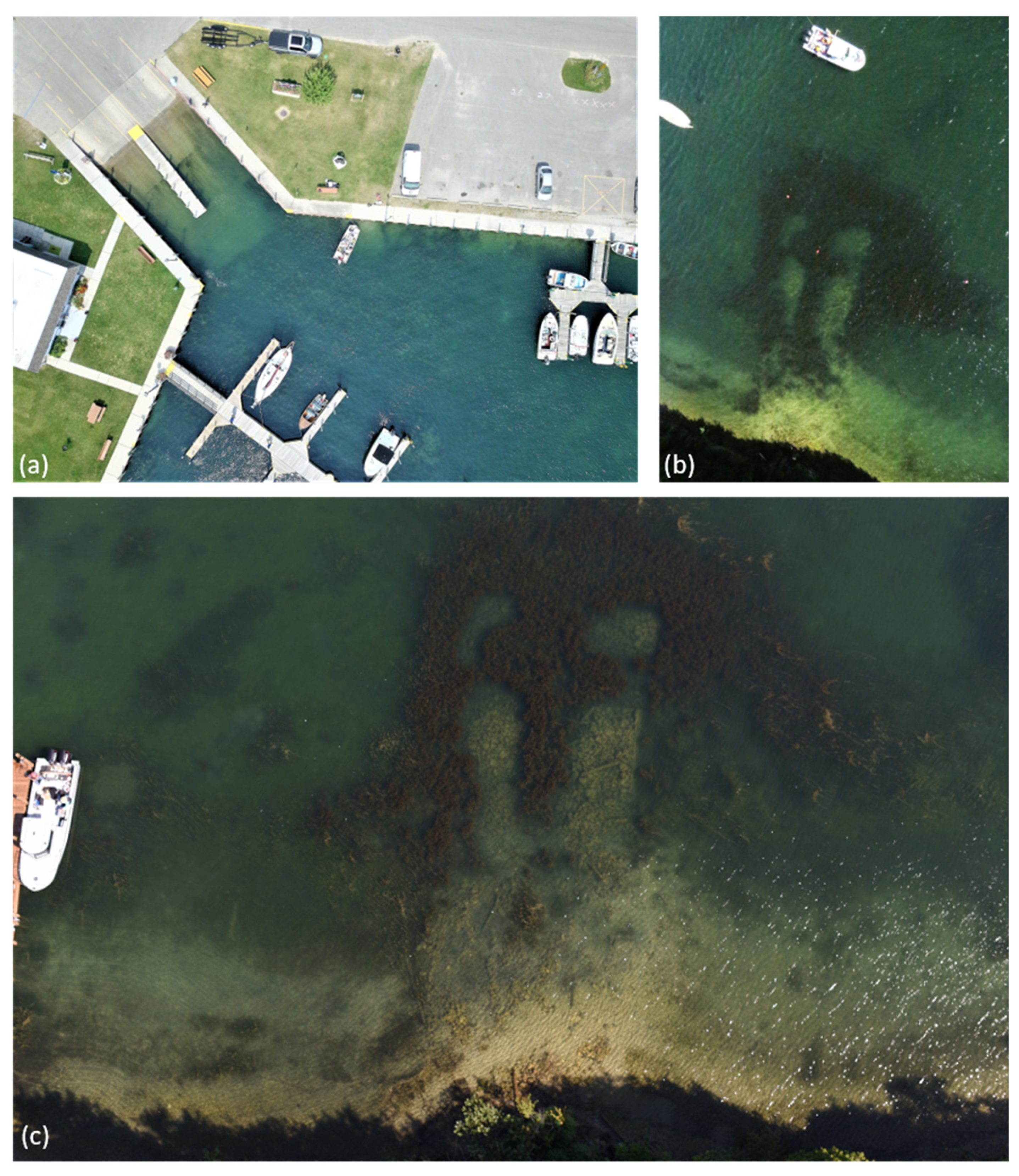
Figure 2 shows an example of three sources of RGB imagery, from the Mavic Pro at Hessel Marina (a), the Canon RGB camera at Howells Dock (b), and the Nikon D810 36mp RGB camera, also for Howells Dock.
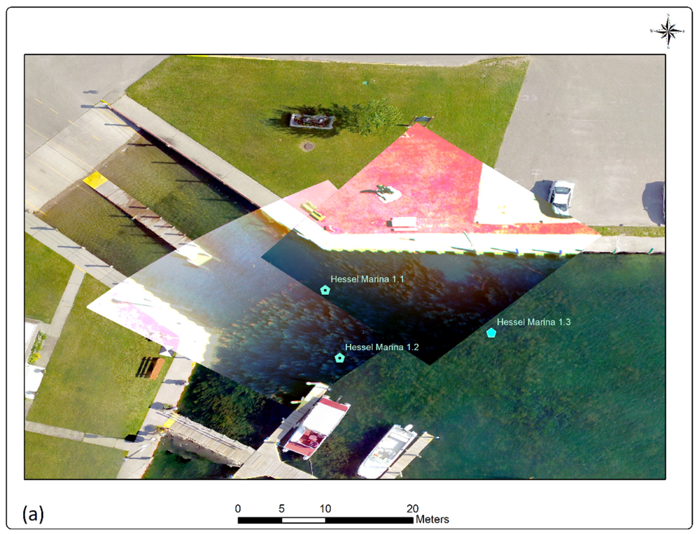
Tetracam imagery consisted of six spectral bands collected at 490 (blue), 530 (green), 550 (upper range of green), 600 (orange), 680 (red), and 720 nm (red edge), with the modified mNDVI calculated from the red-edge and red bands as described in [
26]. The Tetracam was calibrated before each flight against a standard grey reference target provided by the manufacturer for this purpose. The VISNIR system and RGB cameras were not calibrated systems. An example of the Tetracam data collected at the Hessel Marina site in July 2017 is shown in the top part of
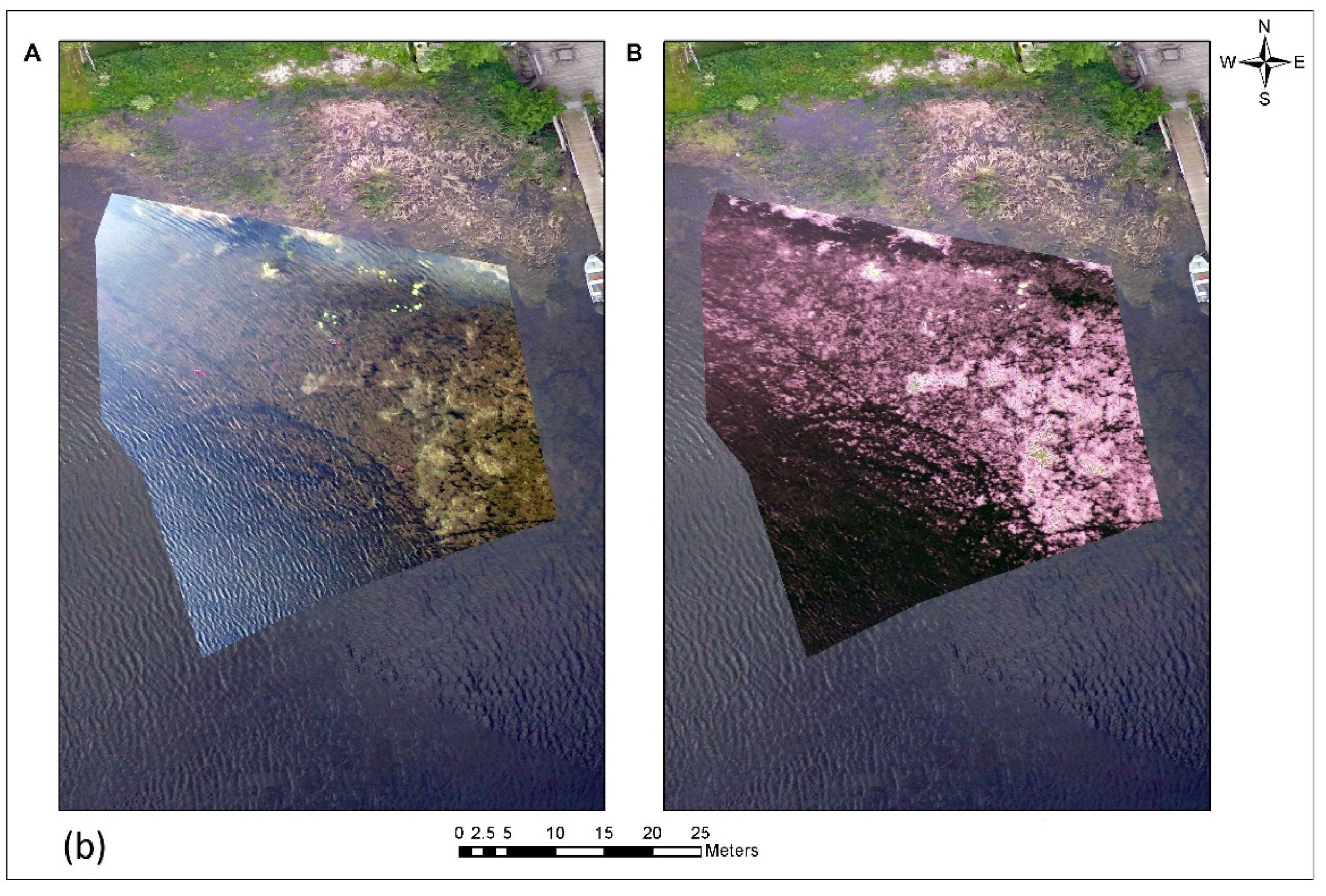
Figure 3, overlaid on an RGB image taken the same day with a Phantom 3A. The Tetracam imagery is shown in color infrared (CIR), with bands 6 (720 nm—red edge), 5 (680 nm—red), and 2 (530 nm—green 1) displayed in the red, green, and blue channels, respectively. Two different views of the VISNIR data are shown in the bottom part of
Figure 3, with the left figure (a) showing RGB imagery and the right figure (b) showing the near-infrared image, with vegetation showing as shades of the more prominent pink color.
Collection and analysis of spectral data at the project sites are described in [
26] with results reviewed here. That study found that a modified Normalized Difference Vegetation Index (mNDVI) using red-edge and red bands was significantly different among dominant vegetation groups using our 2016 and 2017 spectral data, with no difference among months of data collection and no significant interaction between collection month and dominant vegetation group. It appeared that mNDVI was detecting different amounts of SAV biomass, even given the limited water penetration of the red-edge (720 nm) band. mNDVI also appeared to be scale independent and more appropriate for identifying EWM than other species of SAV. Using the six spectral bands alone rarely resulted in EWM being identified separately from other vegetation. As noted in the sensor descriptions, the available multispectral systems included either six bands for Tetracam that could be used to calculate mNDVI or four bands for VISNIR that could be used to calculate standard NDVI. All of these bands were included for image classification in case some bands in addition to mNDVI or NDVI could help provide differentiation for individual sites, if not consistently.
2.2. Water Chemistry Data and Analysis Methods
At each site during each visit, we collected a set of standard water chemistry and light data [
28] to quantify the CPA values at each site and characterize the sites as having lower or higher water clarity. Primary data collected included the following:
Chlorophyll-a concentrations, in mg/m3;
Light intensity, used to calculate extinction coefficient Kd(PAR);
Secchi disk transparency (SDT), in meters;
Depth to bottom, in meters;
Total suspended solids (TSS), in mg/L;
Dissolved organic carbon (DOC) concentration, in mg/L;
Depth to EWM for each collection site, as a range of estimated values;
Percent open water, averaged for each collection site by date.
We derived the following variables to help characterize water clarity:
Depth to 10% light remaining, in meters, which approximates Secchi depth (Dodds and Whiles, 2010);
Depth to 1% light remaining (photic zone), in meters;
1/Kd(PAR);
Percent light remaining at depth of bottom.
The method we used for measuring chlorophyll-a was based on standard methods [
29], including collecting water into 1 L plastic bottles and storing samples on ice until returning to the lab within eight hours. Water was filtered through 47 mm diameter 0.7 µm glass fiber filters, with filters wrapped in aluminum foil and frozen at −20 °C until analysis within a month. Chlorophyll-a filters were extracted in 95% ethanol and analyzed spectrophotometrically following APHA method 10200H.2.b/EPA method 446.0, with calculations following [
30].
To calculate the extinction coefficient of photosynthetically active radiation Kd(PAR), we used a Li-Cor LI-193 SA spherical underwater quantum sensor with a LI-1400 datalogger (LI-COR, Inc., Lincoln, NE, USA), with light intensity values recorded above the surface, immediately below the surface, and every 0.5 m until the bottom was reached, with the bottom depth also being recorded [
31]. The log-transformed light intensity values were then fit to a regression line, with the negative slope of the line being the extinction coefficient. We also recorded Secchi disk transparency depth at each site.
For TSS, we used APHA method 2540B [
29] to calculate the mass of total suspended solids (TSS) in mg/L. Water was collected into 1 L plastic bottles and stored on ice until returning to the lab within eight hours. A well-mixed, measured volume of a water sample, typically 750–1000 mL, was filtered through a pre-weighed 47 mm diameter 0.7 µm glass fiber filter. The filter was heated to constant mass at 104 ± 1 °C and then weighed. The mass of material captured on the filter divided by the water volume filtered is equal to the TSS.
For DOC, we collected water samples in 60 mL Nalgene bottles. Samples were filtered through 0.45 μm membrane filters and frozen at −20 °C until analysis. DOC samples were acidified with hydrochloric acid and quantified using a Shimadzu TOC-VCSN (Shimadzu Scientific Instruments, Columbia, MD, USA).
The depth to EWM was based on visual estimation of the field team to the top of visible EWM growth at each site. The depth to bottom was measured as part of the SDT measurements by dropping the Secchi disc all the way to the bottom.
Percent open water was also based on visual estimation of the field team, with open water defined as areas with no emergent or submerged aquatic vegetation present within the visible water column at each site.
The depth to 10% light remaining is calculated by taking a constant (2.3) and dividing it by the Kd(PAR) value [
32].
The depth to 1% light remaining is calculated by taking a constant (4.605) and dividing it by the Kd(PAR) value [
32].
The percent of light remaining at the depth of the lake bottom was calculated using the formula e
(−Kd(PAR) × (depth to bottom), reported as a percentage (result × 100) [
33].
2.3. Site Type Analysis
Based on fieldwork observations, we expected that at least two types of sites might exist in our study area: sites with relatively clear waters and lower levels of CPAs that reduce water clarity, and sites with relatively darker (more turbid) waters and higher levels of CPAs that result in lower water clarity. For the purpose of this paper, we call sites with higher water clarity “Type A” and sites with lower water clarity “Type B”. We hypothesized that EWM identification methods developed for areas with a lower water clarity (Type A) will work better (be more accurate) in darker waters than in clearer waters and that EWM identification methods developed for areas of higher water clarity (Type B) will work better (be more accurate) in clearer waters than in darker waters. In this paper, we explored whether different image analysis parameters might lead to higher classification accuracy depending on site type. This can be summarized as
Table 2, with our hypothesis that accuracies are higher when classification and water type match:
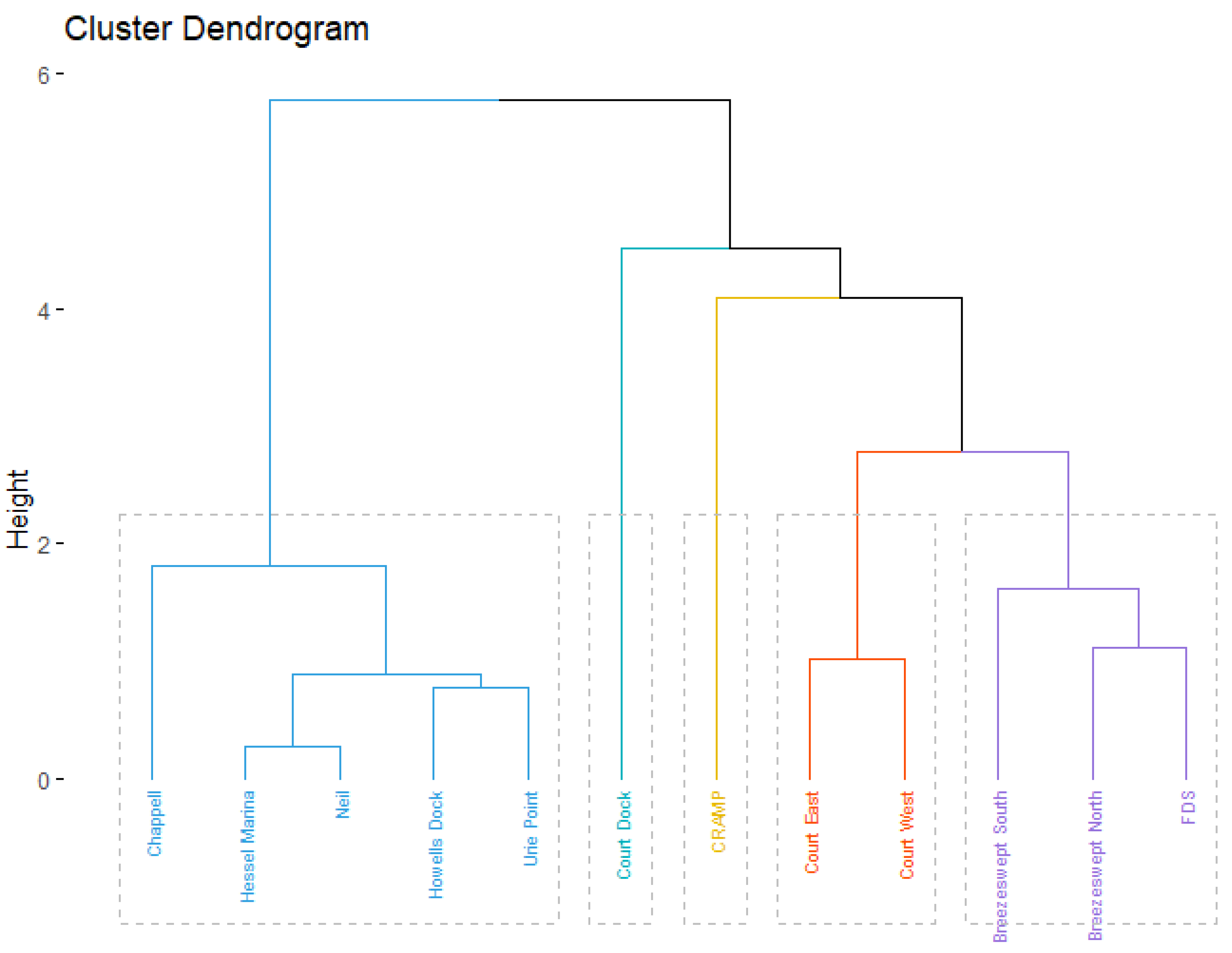
We organized data by site and by date (see
Supplementary Material Table S2). We then averaged light and water chemistry values by site to help understand whether the sites could be clustered into types based on their color-producing agents (represented by TSS, Chl-a, and DOC), with water clarity estimated by the extinction coefficient Kd(PAR).
Table 3 shows the average data, and the data for each individual site by date are included in the
supplementary materials. We used the R cluster package for computing hierarchical clustering [
34] and the factoextra package for visualizing the results [
35], all in R version 3.6.0 [
36]. To investigate the optimal number of clusters, we performed k-means clustering on the site-averaged data initially using 2, 3, 4, and 5 clusters to help understand potential site clusters present in the data. We used the gap statistic method to estimate the optimal number of clusters using the fviz_nbclust function available in the factoextra package. We used the ward.D2 method to compute hierarchical clustering using a Euclidean dissimilarity matrix. The fviz_dend function was used to create a dendrogram to visualize the results of the cluster analysis. As part of site type analysis, we averaged the values of each site according to whether they were lower or higher water clarity and also calculated the standard deviation. Using R, we applied a two-sample
t-test to see if the means were different between the two water types, testing for a normal distribution using the Shapiro–Wilk test and that the variances were equal using the F-test.
2.4. Vegetation Data and Analysis Methods
Field sampling of vegetation type and density was completed through visual estimates, rake tosses, and rake twists, with results recorded on standardized field sheets [
28]. Visual estimate methods and percent vegetation by sampling location were described in Brooks et al. 2019 and based on the Michigan Department of Environmental Quality guidance of 2005 [
37]. Visual estimates were made by an experienced aquatic vegetation expert at the same locations used to create the spectral profiles analyzed for [
26], representing an approximately 3 m radius. In 2016, visual estimates were made in approximately the center of each sampling site and recorded on a field data sheet, and location coordinates were recorded with a Trimble GeoExplorer GPS with sub-meter accuracy. In 2017 and 2018, three marker buoys were placed in the water around each site and three visual estimates were made per buoy in different directions, with locations recorded with the same Trimble GPS and visual estimate data recorded on field sheets. These field sheets were later transferred into a project spreadsheet that documented all three years of field survey vegetation and water sampling data. These data formed the primary source of information for classifying the multispectral UAS-collected images and in assessing accuracy of the classification results.
Rake twists provided a more benthic-oriented sampling of vegetation types than rake tosses. For rake tosses, a rake end was tied to a rope, thrown approximately 10 m, and dragged back toward the boat. Rake fullness was scored on a four-point scale (1, 2, 3, or 4 = found, sparse, common, dense) based on a visual estimation, and vegetation types were recorded by approximate predominance. With rake twists, a rake end mounted on a two-meter pole was thrust downwards into the water immediately off the side of the research vessel [
38]. Vegetation caught in the rake was deposited in buckets for sorting and identification, including predominance on a five-point scale. The macrophytes from each twist rake sample were separated and identified to species using [
39,
40]. Species of
Chara and
Elodea were identified to genus. EWM and hybrid EWM (
M. spicatum x sibiricum) were grouped together, as they are not distinguishable in the field and are difficult to separate [
41]. The samples were dried for 48 h at 60 °C to determine dry weight (see [
5] for more detail).
Photographs of sampling sites were taken with a rugged, waterproof GPS-enabled camera. Photos were generally taken both above and below water to help capture the appearance of SAV and provide supplementary information on species identification.
2.5. Imagery Analysis and Classification
To create geospatial output layers of EWM location and extent, we used the object-based image analysis (OBIA) software eCognition Developer, version 9 [
42]. Recent work, particularly by [
43,
44], has shown promise in applying eCognition’s OBIA capabilities to mapping submerged aquatic vegetation, including EWM, in a riverine environment.
We used eCognition Developer’s multiresolution segmentation tool to create segmentation objects, with mean brightness, means of each band, and mean maximum difference as the classification features for a supervised nearest neighbor analysis. The standard nearest neighbor was applied to all classes. Training data for classification was based on the vegetation data [
28] collected on the same day that we collected UAV imagery mostly using the visual estimate data described above as this provided a similar view to UAV imagery.
Based on initial visual assessment of image segmentation, we modified the scale parameter to develop segmentation objects (polygons) that appeared to capture the extent of submerged aquatic vegetation patches without the polygons being mixed with dissimilar appearing areas. Scale parameter is a user-specified threshold in eCognition where a higher value results in a smaller number of larger segments; smaller values result in smaller, more fine-scale segments. We primarily focused on two scale parameters, one larger and one smaller, to test whether the scale parameter could be optimized for accuracy based on water characteristics. Based on these initial investigations, a scale parameter of 25 (smaller segments) appeared to capture the extent of SAV well for Type A higher water clarity sites, while a larger scale parameter (larger segments) of 50 appeared best at this for representing SAV extent for Type B lower water clarity sites.
We explored whether these different scale parameters might lead to higher classification accuracy depending on site type. We focused on analyzing the impacts on accuracy of these two scale parameters based on water clarity. Other eCognition parameters used for the classification included no differences in weighting for image layers and the default composition of homogeneity criterion with Shape = 0.1 and Compactness = 0.5.
After developing these classification schemes that appeared more appropriate for Type A and Type B sites, we then also applied the classification scheme to the opposite water type. Visual interpretation of classification results was used, informed by field data including estimation of vegetation species present and their extent, with rake toss and rake twist data also helping to verify visual estimate results. We followed the accuracy assessment methods of [
45], including selecting their recommended number of assessment points per classification type and randomly locating those points within each class (such as EWM, open water, etc.) using ESRI ArcMap versions 10.6 and 10.7. Any segmentation polygons used for classification training were not used for accuracy assessment. The number of training polygons varied but was typically approximately 10 for more common classes and about 5 for less common classes.
For each randomly located point in the accuracy assessment, the classifier’s identification was compared to what the field team identified the point as in the vegetation surveys, primarily using the visual estimate data because that represented the uppermost layer of vegetation, which was similar to what the UAS imagery was capturing. UAS RGB orthoimagery, the multispectral imagery used for classification, and location-tagged photos collected with a rugged GPS-enabled camera were also used to determine classification accuracy.
The number of sampling points for the accuracy assessment of classification results was determined using the multinomial distribution described in [
46] as recommended by [
45]. To help understand whether the accuracy of EWM discrimination was dependent on the area of EWM present at a site, the total number of classification points used for accuracy assessment (as recommended by [
45]) are included in our results. Error matrices were calculated for all classifications following [
47].
Applying the two sets of classification parameters developed for Type A and Type B sites yielded two accuracy assessments per classification mapping result. To test the hypothesis that classification accuracy was affected by scale parameter, we applied a mixed linear model in JMP version 14.0.0 (SAS Institute Inc., Cary, NC, USA), with fixed model effects, Scale and Site_type and the interaction Scale*Site_type, as well as a random factor for sampling site to account for the fact that observations from the same site are not independent. Significance for all fixed and random factors was considered at a confidence level alpha value of 0.05. Scale represented whether the accuracy result was based on using the smaller or larger eCognition scale parameter (i.e., 25 or 50 as described above). Site type was determined from the cluster analysis based on CPA at each site as described above. The mixed linear model was run for three different response variables, overall accuracy, EWM producer’s accuracy, and EWM user’s accuracy, using all classification accuracy results, to evaluate whether scale or site type might differ for one or more of these accuracy calculations.
3. Results
3.1. Types of Sites
The TSS values were very low at all of the sampling sites (see
Table 3), with values in the range of 0.0011 to 0.0183 g/L (1.1 to 18.3 mg/L). The Chl-a values were characteristic of oligotrophic conditions (defined as <2.5 mg/m
3, see [
48]), with only single samples at Breezeswept South, Court East, CRAMP, and Howells Dock above 2.5 mg/m
3. The DOC values were relatively high, with the highest values occurring at the sites near Cedarville (averaging 5.06 to 12.73 mg C/L) where a stream (Pearson Creek) empties into Cedarville Bay. Other sites, which do not have a stream near them, had values in the range of 2.57 to 3.02 mg C/L. Reflecting these inputs, the Kd(PAR) extinction coefficient values were highest, indicating the lowest water clarity, for the Cedarville area sites of Breezeswept North, Court Dock, Court East, Court West, CRAMP, and FDS (0.92 to 2.20 /m) but lower for the other, higher water clarity sites of Chappell, Hessel Marina, Neil, Howells Dock, and Urie Point (0.50 to 0.74 /m). The SDT and depth to bottom were highest at the Hessel Marina and Howells Dock sites. The SDT and depth to bottom were the same value at most of the sites (i.e., the Secchi Disk was visible at the lake bottom). The depth to 10% light remaining were sometimes more and sometimes less than the depth to bottom; the photic zone (depth to 1% light remaining) was always more than the depth to bottom. The percent light at depth values varied from as low as 0.4% to as high as 65.6%. The depth at which the EWM was present was often at the surface (0) but could be from 1.4 to 1.8 m (at Neil, for example). The % open water varied from as low as 0% at Court East to as high as 87.0% at Breezeswept South.
Figure 4 shows the results of the five-group dendrogram analysis. The five sites in the first dendrogram branch (Chappell, Hessel Marina, Neil, Howells Dock, and Urie Point) are the same ones that are not near a stream source and that we labeled as Type A high water clarity sites; the remaining sites in the second branch (Court Dock, CRAMP, Court East, Court West, Breezeswept South, Breezeswept North, and FDS) are all close to Pearson Creek with its relatively high DOC waters and were labeled as Type B low water clarity sites. The dendrogram analysis showed that the sites with a higher average DOC (higher light extinction coefficient) could be differentiated into different clusters, but all within the same branch. All sites in the clearer water cluster had k values of below 0.8 m
−1, while all sites in the darker water cluster had k values of above 0.9 m
−1.
With the log transformation of the TSS and Chl-a data, the data for all of the variables were normally distributed. Whether variances were equal for each variable (by site type) was tested using the F-statistic. For data where the variance was equal, the regular
t-test was used; where it was not, the Welch’s
t-test was used. These
t-tests showed that the means between the Type A higher water clarity and the Type B lower water clarity sites were not equal for the DOC, KdPAR, SDT, depth to bottom, depth to 10% light, depth to 1% light, and 1/Kd(PAR) (
Table 4). The means were equal for the TSS, Chl-a, percent light at depth, and percent open water.
The variables where means were not equal are those more likely to be contributing to differences between the Type and Type B water clarity sites. The DOC was the water chemistry variable where the means were not equal. This is likely to affect all of the variables related to water clarity—Kd(PAR), SDT, depth to bottom, depth to 10% light, depth to 1% light, and 1/Kd(PAR).
3.2. Classification Results
We had sufficient project resources and usable multispectral imagery to create classification mapping results for five sites with varying numbers of dates: Breezeswept North (for one date, July 2017), Court East (three dates: August 2016, June 2017, and July 2017), Hessel Marina (one date: July 2017), Howells Dock (three dates: August 2016, August 2017 using two separate images, and August 2018), and Neil (one date: July 2017) for ten site/date combinations total.
As noted, every site was classified using both the Type A and Type B eCognition scale parameters (clear = 25 and dark = 50), resulting in two results per analyzed site and date combination for 20 total classification results (summarized in
Table 5).
Supplementary Materials Section S3 has the complete results for each site/date combination. Included for each result set are representations of the input multispectral image, a background UAS image if available, the classification result with the scale parameter 25, and the classification result with the scale parameter 50. Also included is a description of the site, the vegetation found there, and representative field photos that help describe the site.
We review 5 of the site/date/scale parameter combinations here, out of the 20 available, which are:
Breezeswept North, for July 2017, with Tetracam imagery, and scale parameter = 50;
Court East, for June 2017, with VISNIR imagery, and scale parameter = 25;
Hessel Marina, for July 2017, with Tetracam imagery, and scale parameter = 25;
Howells Dock (image 916), for August 2017, with Tetracam imagery, and scale parameter = 50;
Neil, for July 2017, with Tetracam imagery, and scale parameter = 50.
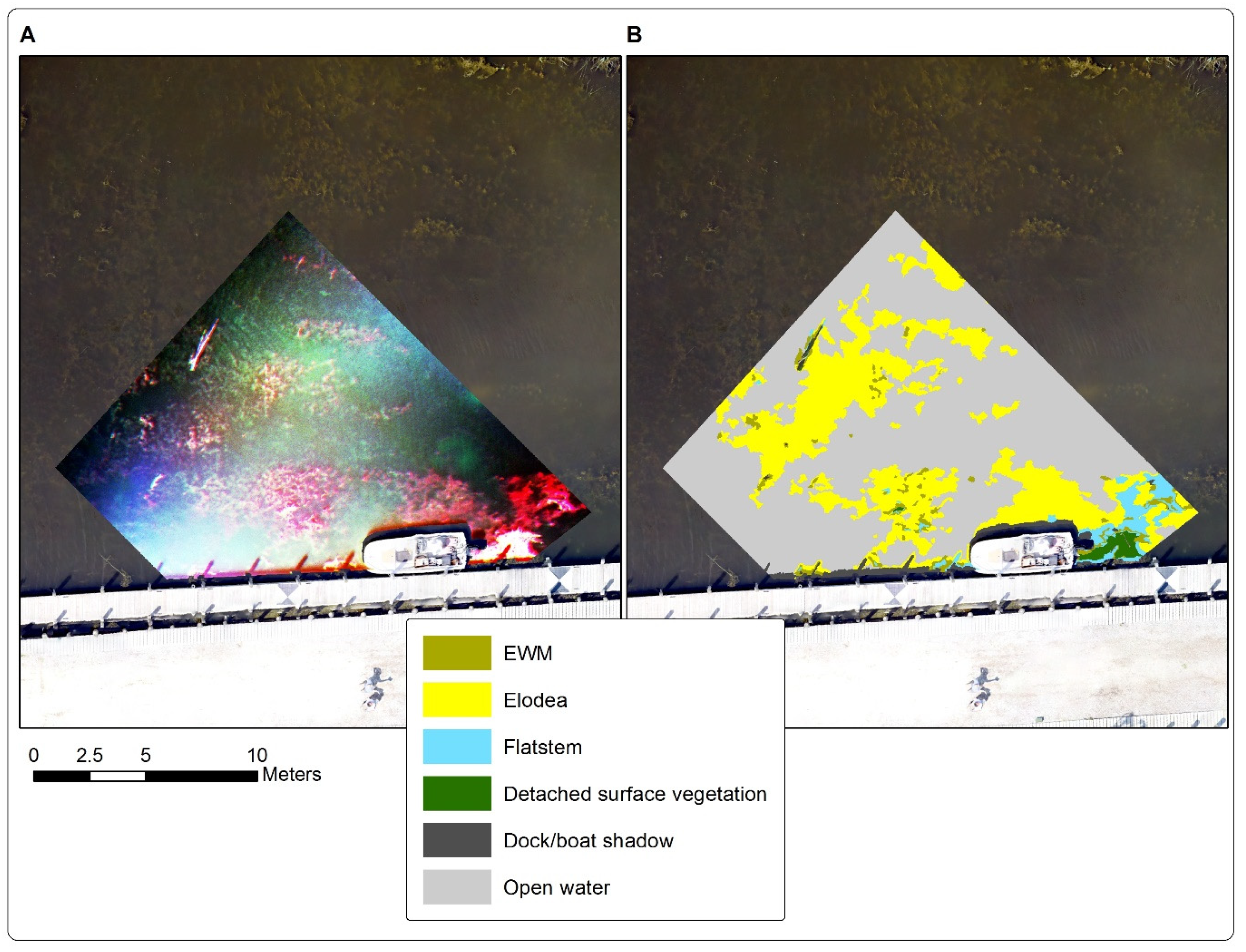
Breezeswept North is a darker water site that was selected as it was the only site with three major taxa of SAV present, with EWM,
Elodea canadensis (Canadian waterweed), and
Potamogeton zosteriformis (flat-stem pondweed). The EWM was also scarcer here than the other four sites, with the Elodea being predominant.
Figure 5 shows the input Tetracam image with a color-infrared display and the classification result using scale parameter = 50.
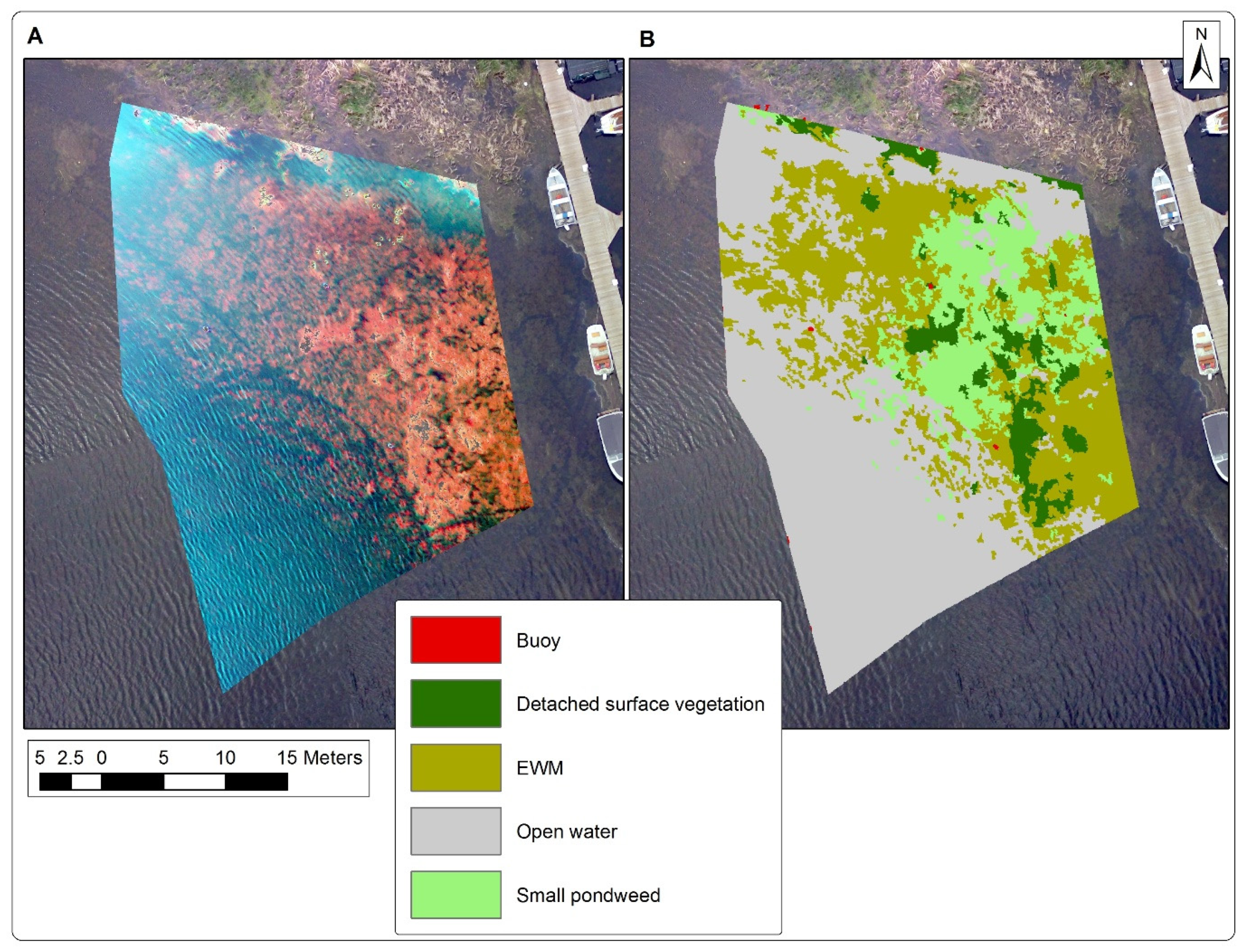
Court East is a lower water clarity site, and the June 2017 date was selected to help demonstrate the results of the classifying imagery from the four-band VISNIR system.
Figure 6 shows these results, with the EWM and
Potamogeton pusillus ssp.
pusillus (small or small-leaf pondweed) present, along with areas of detached SAV floating at the surface.
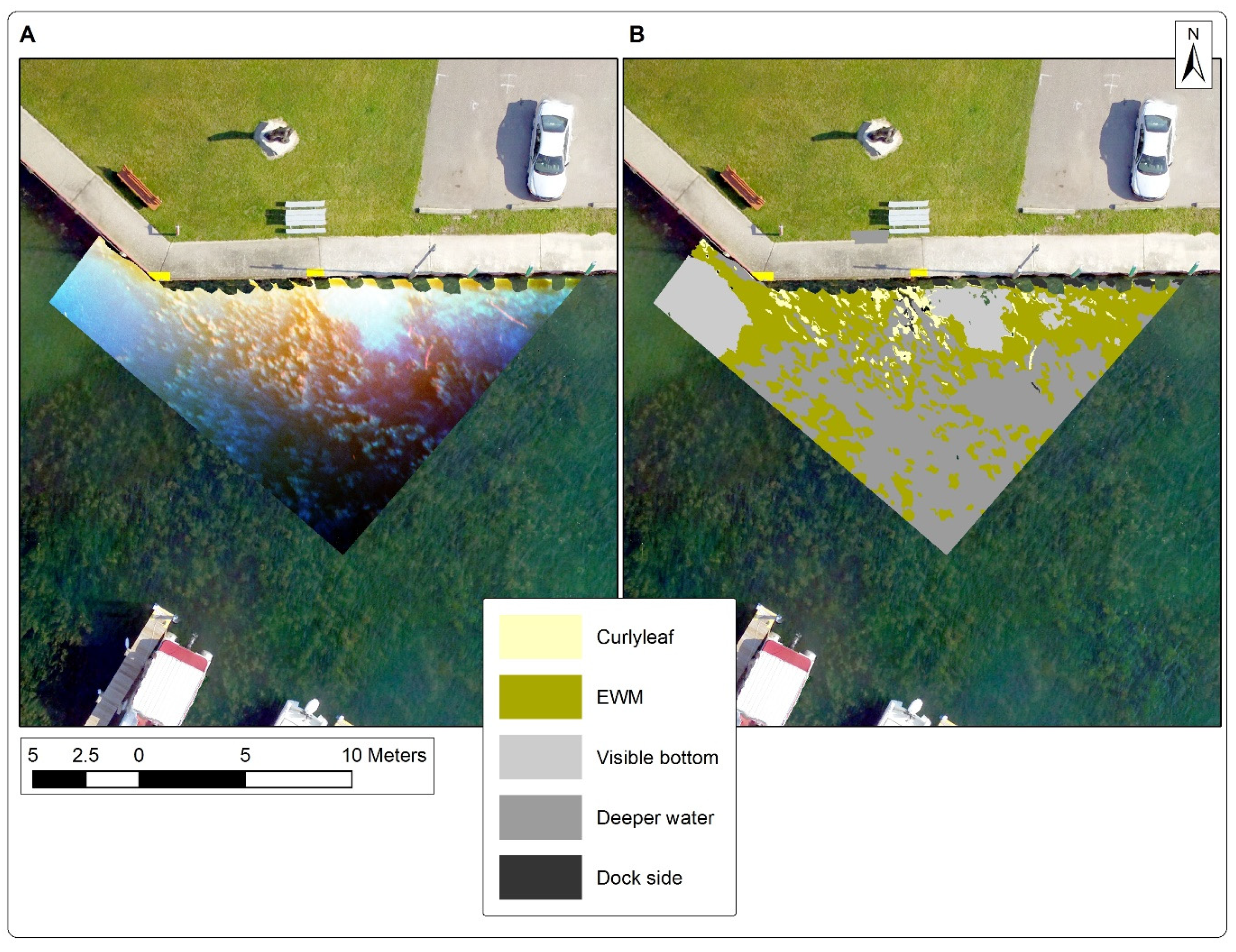
Hessel Marina is a higher water clarity site, with the July 2017 result selected because of the presence of two invasive aquatic plant species, EWM and
Potamogeton crispus (curlyleaf pondweed).
Figure 7 shows the Tetracam input image and classification result for scale parameter = 25. This image was taken a few days before treatment to reduce EWM growth was started with a native fungus and was intended to form a baseline for monitoring treatment effectiveness.
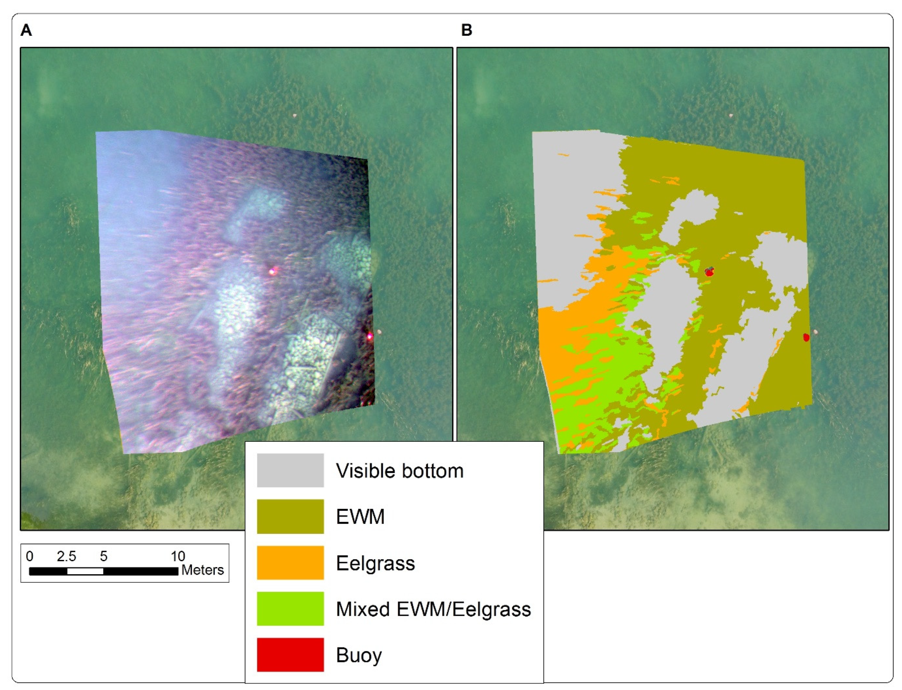
The Howells Dock input Tetracam image and resulting classification with the scale parameter = 50 for August 2017 are shown in
Figure 8. This higher water clarity site did not undergo treatment for EWM removal during the study period of 2015–2018. This result was chosen because of the presence of both eelgrass (
Vallisneria americana, also known as water celery or tapegrass) and EWM. In a transition area, the presence of both eelgrass and EWM necessitated the use of a mixed EWM/eelgrass class type.
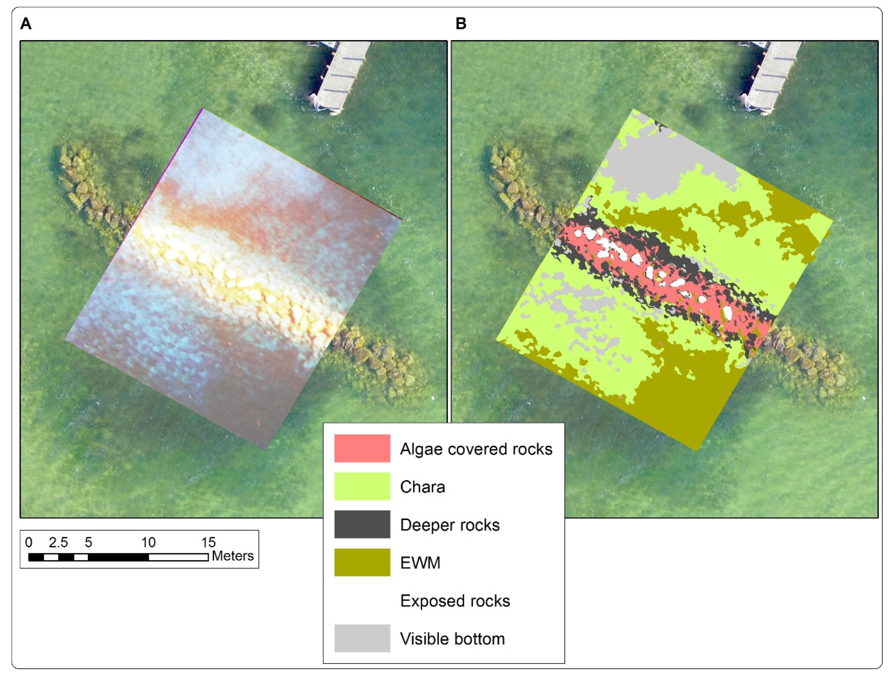
Neil is a higher water clarity site immediately west of Hessel Marina, with the July 2017 result shown. This example was included because the two types of SAV present,
Chara and EWM, were both deeper than the SAV at other sites, at approximately 1.75 m beneath the surface in 2.4 m of water. This provided the opportunity to determine if
Chara and EWM could still be differentiated in a deeper water site where the plants were in a relatively short growth form, not near the surface.
Figure 9 shows the Tetracam input image and the classification results for scale parameter = 50. The presence of exposed, algae-covered rocks just beneath the surface and a visible sandy bottom also provided a useful example of the need to have multiple non-SAV classes to complete the classification.
3.3. Error Analysis
The overall accuracies varied from a low of 60.0% at Hessel Marina in July 2017 with the scale parameter = 50 (30/50 interpretation points correct) to a high of 97.7% at Court East in July 2017 with the scale parameter = 25 (43/44 correct). The lowest EWM producer’s accuracy was 0.0% at Breezeswept North in July 2017 with the scale parameter = 25, but this was at a site with a limited presence of EWM and 0/2 interpretation points correct; excluding this site, EWM producer’s accuracies ranged from a low of 56.0% at Court East in June 2017 (for the only pair of classifications conducted from the VISNIR imagery) with the scale parameter = 25 (14/25 correct) to three sites having a high of 100%: at Court East in July 2017 with the scale parameter = 25, with this site having a mixed EWM/Elodea class (14/14 correct); Howells Dock in August 2016 with the scale parameter = 25 (19/19 correct); and Howells Dock in August 2018 for scale parameters 25 and 50 (17/17 correct for the scale parameter = 25 and 19/19 correct for the scale parameter = 50). Excluding Breezeswept North again, where EWM was present but scarce, EWM user’s accuracies ranged from a low of 51.9% at Court East in June 2017 with the scale parameter = 50 (14/27 correct, for the only VISNIR classification pair) to two sites with a high of 95.0%: Howells Dock in August 2016 with the scale parameter = 25 (19/20 correct) and Howells Dock, image 916, in August 2017 with the scale parameter = 25 (19/20 correct).
Average accuracies using all 20 classification results were 78.1% for overall accuracy, 74.5% for producer’s accuracy for EWM, and 75.6% for user’s accuracy for EWM. The average accuracies for the 18 out of 20 classifications that used Tetracam multispectral data, which was used to calculate the mNDVI, were 79.3% for overall accuracy, 75.6% for producer’s accuracy, and 77.4% for user’s accuracy. For the 2 out of 20 classifications that used the VISNIR data, which was used to calculate the standard NDVI, the average accuracies were lower with 67.9% for overall accuracy, 64.9% for producer’s accuracy, and 59.3% for user’s accuracy.
These results can also be summarized to match the format of
Table 1, with the averages plus or minus one standard deviation (see
Table 6). For the Type A sites with greater light penetration on average, the average accuracy for the Type A type classification with the scale parameter = 25 was not higher than that for the lower clarity Type B classification with the scale parameter = 50. For the Type B sites with lower light penetration on average, the accuracy was higher using the Type A type scale parameter than the Type B type scale parameter.
The mixed linear model was designed to understand whether the classification accuracies were significantly affected by the scale parameter.
Table 7 shows these mixed model results.
None of the results were significant at the p = 0.05 level. Neither the scale parameter nor the site type had a significant effect on overall accuracy, and there was not a significant interaction between the scale and site type.
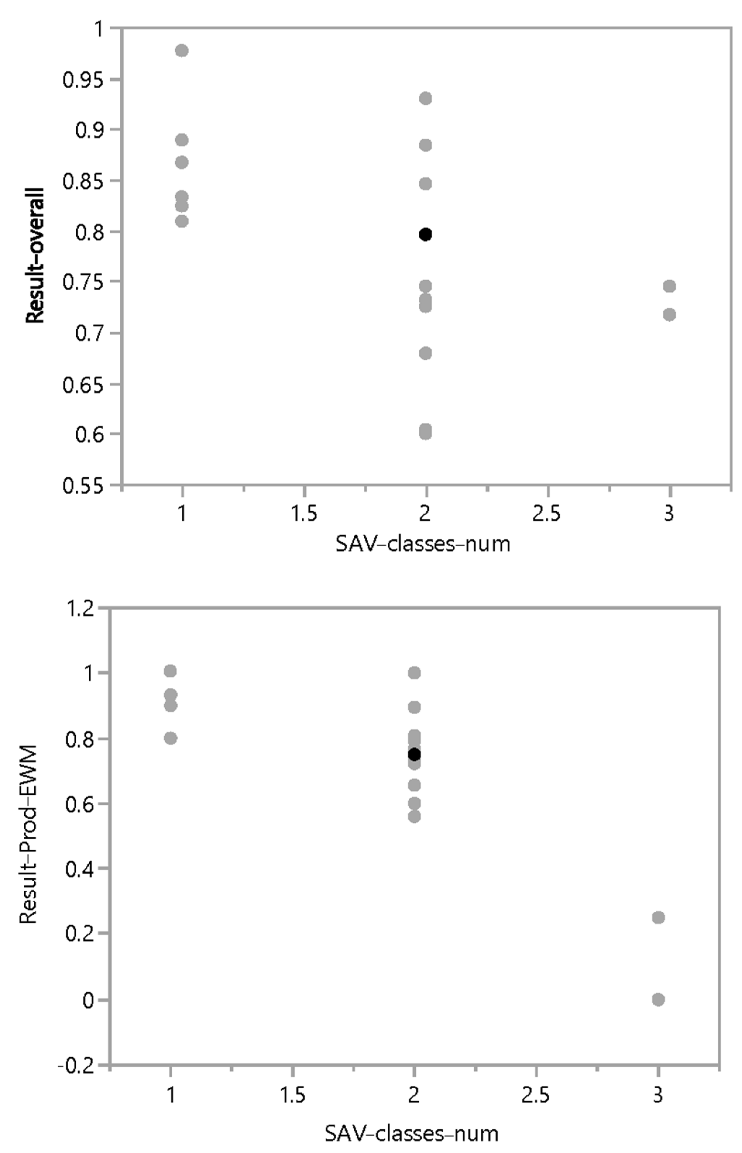
As the classification process was carried out, it seemed possible that the accuracy was influenced by the number of SAV species classes that we were attempting to map for each image. The number of SAV classes ranged from one (such as at Howells Dock in August 2018 when only EWM was mapped based on vegetation field surveys) to as many as three (at Breezeswept North, with EWM,
Elodea, and flat-stem pondweed all identified and mapped,
Figure 8). To test this, we used the Kruskal–Wallis rank-sum test in JMP version 14.0.0 to compare the accuracy as the response variable among groups with 1, 2, or 3 SAV classes with post hoc Dunn tests to compare among the three groups. We ran separate tests for the overall accuracy, producer’s accuracy, and user’s accuracy.
For the overall accuracy, the Kruskal–Wallis test indicated that the groups were significantly different (χ
2(2) = 6.26,
p = 0.044), but the post hoc Dunn tests did not identify any significant differences between the groups (
Figure 10, top).
For the producer’s accuracy, the groups were again significantly different (χ
2(2) = 11.45,
p = 0.0033), and the Dunn test indicated that the accuracy was significantly higher for classifications with one class vs. those with two or three, but there was no difference between classifications with two or three groups (
Figure 10, bottom).
For the user’s accuracy, there was no significant difference in the classification accuracy based on the number of SAV classes present (χ2(2) = 0.26, p = 0.88).
3.4. Discussion
3.4.1. Accuracy Discussion
Accuracies for classified multispectral UAS images are higher than previously reported in the literature for the identification and mapping of different types of SAV. We obtained an average overall accuracy of 76.7%, a producer’s accuracy of 78.7%, and a user’s accuracy of 77.6% across the 20 classifications. With the Tetracam results, we were able to exceed the 61% maximum overall accuracy noted in [
43] on a consistent basis across both dark and clear water sites. The authors of [
49] compared the field data of emergent and submerged aquatic vegetation to distribution mapping created using remote sensing and echo-sounding techniques. Echo sounding produced the most comparable results to field data, with 71% producer’s accuracy and 73% user’s accuracy for non-canopy-forming SAV species (such as eelgrass and
Chara), but they were not able to map canopy-forming SAV such as
Myriophyllum spp. They tested an early multispectral airborne sensor with eight bands ranging from 390 to 1100 nm (ultraviolet edge to near-infrared) but only achieved 18% overall accuracy with 7 m pixel resolution and concluded that image-based remote sensing was “expensive and problematic”. While they noted problems with the water color, including turbidity, we were able to identify EWM in sites such as Court East where it was found a meter below the surface and at two meters below the surface in clear water sites such as Howells Dock.
The authors of [
43] note that there are many factors that affect the overall accuracy for SAV identification, including band alignment problems for multispectral imaging devices and the radiometric impacts of sky factors (sunglint, specular reflection, shading). We focused our data collections as much as possible to within two hours of solar noon, which helped reduce these issues. We did see some alignment issues, particularly in the red-edge bands, but these did not appear significant over the scale of the images being analyzed, at least based on the mapping accuracies we obtained. We found that clear sky, sunny days with low winds were optimal for obtaining images where the SAV was most easily visible, while cloudy days produced a large amount of cloud reflectance on the water surface and limited light penetration that made SAV identification much more difficult. We eliminated all of the imagery collected on overcast days from our analysis because of these issues; therefore, this issue should not affect the results and analyses we present here.
The quality and quantity of field data also impacted our ability to create relatively accurate SAV mapping results. The authors of [
43] compared their OBIA-derived results to manually delineated class boundaries and types to assess accuracy and noted that this can have limitations, as manual interpretation is not error-free. We found that above-water and below-water photos, taken with a waterproof digital camera with GPS capability, were very important for evaluating multispectral imagery, especially when referenced to standardized recording of visual estimates of percent cover by SAV species. After our first year and initial attempts to classify the collected imagery, we had found it challenging to relate the visual interpretation (and other vegetation estimates) to specific locations in the imagery, despite recording the position of the boat during field visits. We found that deploying numbered buoys, and being able to see those in UAS imagery, made this process much easier, especially when significant time (months or years) could sometimes go by between field visits and the final image classification and accuracy assessment. We recommend the adoption of these types of marker buoys when using UAS imagery to identify SAV taxa and other applications with a similar scale. As we recorded the locations of the marker buoys with a Trimble GeoExplorer 6000 GPS unit, these could also serve as an additional source of positioning information for orthophoto georeferencing, along with the GPS data embedded in the UAS aerial images.
We also found evidence for an effect of the number of SAV classes on the overall and producer’s accuracy. Sites with two or three species of SAV produced lower accuracy results than sites with just one SAV type to identify for the producer’s accuracy, and the difference was also evident among groups for the overall accuracy. With multiple SAV types, there is the potential for them to be spectrally similar, at least with the multispectral sensors deployed in our work [
19,
26]. With only one SAV class, we were generally only trying to differentiate it from open water or uncolonized bottom substrate, which is easier to accomplish due to larger spectral differences. Our methods have the greatest applicability if the purpose of EWM identification is to map its extent in underwater stands where it is predominant. This would be most useful when tracking changes in its extent due to management efforts that focus on EWM-dominated stands.
3.4.2. Light Penetration, Water Clarity, and Color-Producing Agents
The limited penetration of near-infrared light into water is well known, with the absorption coefficient of water rising rapidly between 700 and 750 nm [
50], and the penetration can be further limited by higher CPA values. With an mNDVI apparently important for identifying EWM from other SAV taxa, these could be expected to reduce our ability to identify this species. However, no site used in our mapping analysis had depths greater than 2.97 m (
Table 3), and the depth to the top of the EWM plants was never greater than 2.0 m and was normally less than 1.25 m. At every site except for Court East and Court West, the depth to 10% light remaining exceeded the depth to the bottom, and except for Court West and CRAM, there was more than 10% light remaining at the bottom depth (
Table 3). In reviewing the imagery visually, we could always identify where the EWM was present in the imagery for the five sites used for multispectral image classification. For these reasons, the mNDVI was effective in identifying EWM with relatively high accuracy in our study, even with the limited penetration of near-infrared light.
Despite the clustering of sites based on the differences in water clarity, it is important to note that all of our sites have relatively clear water, with average k values of 0.5010 to 2.1960. While [
43,
44] do not report a light extinction coefficient for their river site in Belgium, values for other waters indicate that our nearshore areas of the Les Cheneaux Islands were relatively clear. For a shallow, turbid reservoir in Texas, [
51] report k values of 2.49 to 7.93 m
−1, while values up to 8 m
−1 were reported in eutrophic Lake Okeechobee, FL, depending on the season and lake location [
52]; our values are more similar to Lake Mendota in Wisconsin which have been reported in the range of 0.35 to 0.85 m
−1 [
53].
With SAV, we have been attempting to measure the presence and extent of specific species at sites that have a greater variability in the sensing environment than terrestrial sites. The atmospheric correction of the imagery of terrestrial areas is a standard procedure, especially for satellite imagery, but we are dealing with apparent optical properties of water affected by the CPAs and the inherent optical properties affected by the absorption and backscatter of the light signal that gets attenuated. The authors of [
43] noted that standard targets of 85% accuracy are based on terrestrial environments but are more challenging in aquatic environments due to these types of complication factors. In our sites, we have areas with higher DOC values, most likely because of a local creek that drains wetland areas, while sites further away without a local DOC source have higher water clarity. Even without DOC, absorption, backscatter, and surface glint make aquatic remote sensing more challenging [
32,
54]. In sites with higher CPA values, we anticipate that these may alter the spectral signature and mNDVI values of EWM, complicating classifications in lower clarity sites.
3.4.3. Site Types
The cluster analysis showed that we had two types of sites based on the water chemistry data that were collected: those with relatively high water clarity and those with relatively low water clarity. This informed our classification methods, with the idea that a smaller scale parameter was more appropriate for high water clarity sites and a larger scale parameter was more appropriate for dark water sites. However, classification accuracy did not differ significantly between the higher and lower water clarity sites in our analyses, with some local variation. We had expected that the scale parameter of 25 would produce more accurate results for clear water sites and the scale parameter of 50 would produce more accurate results for dark water sites. This was based largely on a visual impression from the initial classification results that a smaller scale parameter appeared to capture finer details in the extent of the SAV more accurately than larger ones. It had seemed that greater detail was visible for the SAV areas in high water clarity sites and that the smaller scale parameter would help capture this. These more detailed features could then be resolved into image objects representing areas of SAV, rather than treating each pixel individually.
For the lower water clarity sites, SAV areas appeared to be less distinct in early classifications, with DOC being the primary CPA affecting water clarity here. However, this was not borne out when all of the classifications and the accuracy assessment were complete, as shown in
Table 6. Indeed, the mixed linear model results showed that the scale parameter was not associated with a significant difference in the overall, producer’s, or user’s accuracy. It may be that each SAV type has its own optimal scale parameter for the highest accuracy results; this idea has been investigated for terrestrial land-cover types [
55]. Scale parameters are designed to help reflect the landscape heterogeneity captured by imagery [
56], and further investigation of how this parameter can best be used to help identify specific SAV species of interest may be warranted. It appeared that the smaller scale parameter enabled a more precise selection of training areas for classification, but this could also mean that inherent variability within a cover class could be missed. This may be what occurred with the large visible differences in the extent between the maps created using the two scale parameters for the flat-stem pondweed at Breezeswept North, the small pondweed at Court East in June 2017, and the deeper rocks class at Neil.
3.4.4. Biomass
The authors of [
57] noted that percentage cover, percentage volume, and dry weight biomass mass could be strongly correlated (R
2 range of 54–96%) for SAV in shallow rivers, with seasonal and site variations in these relationships. We have previously demonstrated that percent cover can be reasonably related to biomass for SAV in our
Cladophora algae remote sensing work that used Landsat data to map the SAV extent with 83% overall accuracy across Lakes Michigan, Huron, Erie, and Ontario [
58,
59]. Relatively accurate mapping of EWM could potentially be used to estimate EWM biomass and how this could change when EWM undergoes management methods.
4. Conclusions
Multispectral UAS-enabled sensing of a specific invasive aquatic plant, Eurasian watermilfoil, was demonstrated as being possible through this research, including when it was mixed with other taxa. The average accuracy we obtained for the identification of different taxa of SAV is higher than previously reported efforts for SAV mapping and shows promise for the multispectral UAS-enabled identification of EWM extent as part of SAV management efforts.
We found that the inclusion of the mNDVI appeared useful in identifying EWM, most likely because this index is sensitive to green vegetative biomass. Despite limited penetration of the red, red-edge, and near-infrared wavelengths into the water column, we found sufficient penetration that multispectral sensing including a red-edge or near-infrared sensitive camera system could help identify SAV. This was demonstrated where EWM was present in the first meter of water at sites with higher DOC concentrations or the first two meters at relatively clear water sites. The ability to detect greater or lesser amounts of biomass in the water column likely contributed to our relatively high accuracy results for SAV identification. In [
19,
26], we found that additional spectral bands were more likely to lead to reliable EWM identification, and the exploration of the specific wavelengths in the red to near-infrared that help identify shallow-depth SAV species is recommended.
With multispectral sensors now deployable onboard UASs on a practical basis, together they can be a valuable tool for ecologists and aquatic managers wanting to understand the extent of specific species of SAV, such as EWM, particularly where the species is dominant in the area of interest. With the dominance of SAV species changing year by year, as seen at some of our sites, UAS-based methods can provide information on the variability of these sites. Future research could compare additional sensors and remote sensing platforms to produce detailed results in time periods useful for field monitoring and management. We expect that our methods will be most applicable to monitoring the effects of the anthropogenic management of aquatic vegetation, which may lead to rapid changes in SAV biomass, extent, and composition.


 ,
, 


