1. Introduction
Widespread international trade exchange and travel has allowed many species to spread to new habitats. If this process takes place within the natural geographical range of habitation for a species, it is called ecological expansion, while when this process starts to cross geographical barriers, it is called invasion or geographic expansion [
1]. Plants naturally increase the area they cover while invasion occurs rapidly based on anthropogenic channels of migration [
2]. The increase in anthropopressure causes an increase in alien invasive species generating transformations of the natural habitats leading to the depletion of biodiversity. This is due to wider tolerance to environmental conditions (e.g., access to sunlight, water, nutrients) of invasive plant species. Moreover, invasive species often transform their habitats by releasing chemicals into the soil that limit the sprouting of other plants or change the structure of the soil to meet their own trophic needs. The appearance of new plants determines the presence of new parasites and pathogen carriers that pose a real threat to the habitat, including the generation of new allergens. A special case of threat to human health and life is Sosnowskyi’s hogweed (
Heracleum sosnowskyi), whose furanocoumarins can cause serious burns to the exposed skin. The proliferation of plants, including the root systems, deforms and destroys the gas, water, road and rail infrastructure and also leads to a reduction in yields in agriculture and forestry [
1,
3,
4]. It is estimated that the costs of protection of European Union countries is up to EUR 12 billion per year [
5].
Traditional methods of plant species mapping rely on field identification of plants on monitored surfaces in given transects. The main disadvantages of this solution are: time-consuming and costly field research, the locality of activities and the inability to thoroughly examine larger areas, the subjectivity of the expert’s assessment and the need to aggressively extrapolate findings into larger areas. The field measurements are then interpolated, which can lead to imprecision of the resulting maps. On the other hand, remote sensing methods enable quick and objective identification of invasive and expansive plant species even in large and inaccessible areas. The use of airborne hyperspectral remote sensing, which offers high spatial, spectral and radiometric resolutions, can identify even small plant patches, which is crucial in controlling new invasion and expansion. The research activities started about 20 years ago in the USA [
6,
7]. Since then, many sub-pixel classification algorithms have been tested around the world in order to optimize species mapping [
8,
9,
10,
11,
12]. An example is the mapping of the
Solidago altissima based on airborne AISA hyperspectral images with high spatial (1.5 m) and spectral (8.9 nm) resolutions on moist tall grassland in the SE Watarase wetland [
9]; authors constructed generalized linear models (GLMs) with binomial errors and a logit link function to identify the American invasive species. As input data, a field-verified set of presence–absence percentage cover and eight minimum noise fraction (MNF) bands (second to ninth), which were reduced to the three most informative: the second, fifth and ninth MNF bands. As a result, spatial distribution of the
S. altissima with user’s and producer’s accuracies ranged from 80.0% to 83.3%, with an overall accuracy of 81.7% [
9]. Research on the identification of invasive and expansive plant species conducted in recent years was focused mainly on machine learning methods, such as support vector machines (SVMs) [
13,
14,
15] and random forest [
16,
17,
18]. For example, The SVM algorithm and the recursive feature elimination (SVM-RFE) approach were used to map the species
Solanum mauritianum in KwaZulu Natal (eastern parts of South Africa) with an overall accuracy (OA) of 93% on selected 17 hyperspectral bands of the AISA Eagle image [
19]. The random forest algorithm and 25 MNF bands of HySpex images for mapping the species
Spiraea tomentosa in the Lower Silesian forests in Poland was used to obtain an F1-score accuracy for the species of 83% (OA—99%) for September’s images and an F1-score of 77% (OA—99%) for August’s [
20]. Most studies indicate the need for methods that reduce the spectral space of hyperspectral imaging, e.g., principal component analysis (PCA) and minimum noise fraction (MNF), in order to reduce the data volume and shorten the data processing time [
21,
22].
An interesting comparison of different land cover classes [
23], including different types of grasses (healthy, stressed and synthetic) based on hyperspectral images (144 bands, 380–1050 nm, 2.5 m pixel size) and machine learning algorithms [
24]: Matched Subspace Detection (MSD), Adaptive Subspace Detection (ASD), Reed-Xiaoli Detection (RXD), Kernel MSD (KMSD), Kernel ASD (KASD), Kernel RXD (KRXD), Sparse Representation (SR), Joint Sparse Representation (JSR), Support Vector Machine (SVM), authors’ customized Convolutional Neural Network (CNN) [
25]. The training data sets oscillated around 190 pixels, and test samples 505–1056 pixels for vegetation targets. The best results (overall accuracy (OA) of 15-class classifications) were acquired for following algorithms: JSR (86.86%), CNN (86.02%) and SVM (86.00%) [
25]. Comparable results were acquired by Li and Stein [
26], who based on GF2 (2.5-m multispectral and 0.78-m panchromatic bands) and ZY3 (6.78-m multispectral and 2.38-m panchromatic bands) satellite images used a deep learning method based upon UNet [
27], Bayesian classifier (derived via Graph Convolutional Networks—GCN) Random Forest and Support Vector Machine. The best overall accuracies oscillated around 85.0–87.5% for Bayesian classifications (combining spatial composition features and structural features), 75.7–80.0% for SVM and 67–68% for RF, but for green areas identified on GF2 images user accuracy achieved 0.93 ± 0.06, but for ZY3 images: 0.63 ± 0.12 (grasses) and 0.95 ± 0.06 (trees) [
26].
In the case of expansive and invasive plants, the most important element is the appearance of new beachheads of invasion, which do not cover large areas of the ground. These plants, depending on their density with background plants, create spatially and spectrally differentiated patches; hence, the difficult element is to create representative classification datasets for training and verification. The solution is to use an iterative classification method, which consists of many independent classifications, and for each of them to use reference from field-verified polygons. This allows for the analysis of various scenarios of the tested plants against the background of the environment. The problem remains; Which result represents the spatial distribution of the examined objects? Iterative accuracy assessment methods are also increasingly used to obtain more reliable results [
28,
29,
30]. The accuracy of maps presenting the spatial distribution of valuable communities and habitats, and on the other hand species posing a threat to biodiversity, is often the basic information for making environmental decisions; hence, the process of mapping and assessing the quality of the final map is a key issue [
29], and mapping invasive and expansive plants, which adopt many strategies, e.g., faster development compared to surrounding species or longer rhizome growth allowing for faster occupation of new areas. Such adaptations create heterogeneity of the species composition of invasive/expansive plants with indigenous species, which in the following years may be eliminated by those with wide ranges of environmental tolerance, hence the need to analyze hyperspectral images in multiple iterations and attempt to evaluate individual pixels according to randomly selected patterns that have been verified in the field, which can lead to analysis of a wider spectrum of different cases [
11].
The problem with the iterative accuracy assessment approach is the multitude of potential results, which forces the author to choose a version for presentation and later processing. There may be a multitude of criteria for such a choice, but it is difficult to take advantage of the wealth of information provided by, for example, 100 resulting images obtained during the analysis. The approach we suggest tries to solve this problem; in addition, our solution allows the researcher to make decisions based on the obtained results, which releases the researcher from performing the so-called best guess because the main idea when creating maps is to provide true information about the distribution of objects in the studied area. This problem is exacerbated by the use of methods based on iterative image classification with the use changing training/validation sets. As a result, n images are obtained after classification, each only an approximation of the real spatial distribution of the classified objects. Additionally, it is not obvious, despite the use of various solutions, which of these n results should be used for the production of the final map.
In summary, produced high-accuracy invasive species maps are usually based on extensive field research or UAV-based multispectral or airborne hyperspectral images, which offer a local range of analyses [
31,
32]. Satellite images show the roughly estimated extent of invasive species habitats [
33,
34]; however, satellite images can be used to prepare and frequently update maps based on phenological properties, allowing the dispersal of seeds and the growth of underground rhizomes to be counteracted faster, e.g., by mowing inflorescences. The authors mainly use machine learning methods (SVM, RF), which are widely available through libraries in open programming languages. Hyperspectral images or a combination of satellite data (Sentinel-2, WorldView) with additional data offers high overall accuracy (over 80%), and individual species are identified with producer’s accuracy of 60–80%, using additional data, e.g., multitemporal, additional high-resolution images, vegetation indices and products from the airborne laser scanning (ALS) models. Depending on the species, accuracy of above 90% can be achieved [
33,
34], but the problem is the spectral variability of invasive species and the surrounding plants, which are prone to change due to agriculture activities, e.g., mowing and grazing, which causes changes in the proportion of the reflected spectrum from the soil, blooming flowers or dry blades of grass. All these elements make it difficult to identify invasion routes, but regular monitoring can identify changes [
35]. Therefore, monitoring of invasive plants should be based on regular image acquisition, and the iterative method can be used to check the pattern of land cover of a given area. It generates a large number of maps representing different configurations of randomized acquired training patterns, which should be systematically analyzed in order to select the optimal set of pixels representing invasive species occurring not only in homogeneous areas constituting the core of the lobe but also individual pixels representing the beginning of the invasion. Our work focuses on the transformation of
n classification images into a reliable map of the spatial distribution of selected invasive and expansive species. Moreover, when developing our solution, care was taken not to overestimate the result. Therefore, this paper presents a new method of combining post-classification results into usable map and how many times a research target was identified on a given area based on randomized selection of classification patterns, which were field-verified, as well as the validation set. Our previous work [
32] focused on the image classification method, whereas this one aims to address issues that result when one has multiple seemingly equivalent post-classification images. Our aim was to determine the most suitable approach for map creation. We decided to follow the method shown in our previous paper because it was proven suitable; hence, we outline post-classification image processing in this paper without explaining in detail the classification methodology we followed. The solution provides for the underestimation of classes and actively takes care not to overestimate them. The presented method consists of a multiple-process hyperspectral image classification, counting the occurrences of individual species in each pixel, thresholding the resulting frequency images and subjecting them to generalization.
2. Materials and Methods
Methods shown in this paper are a continuation of our previous work regarding mapping of invasive and expansive plant species [
32]. Optimization of classification parameters and scenarios, including testing of different classifiers, sets of training and testing patterns were described in the previous manuscript; based on our experiments it was determined that it is preferable to use MNF bands instead of spectral bands. Additionally, we used 300 pixels per class in the training dataset and employed the SVM RBF algorithm as it was shown that this combination of parameters results in the most accurate results. This paper focuses on explaining steps required to produce a map given set of results (
Figure 1).
2.1. Research Area and Objects of the Study
The research area is located in Southern Poland near Malinowice town covering a valuable agriculturally used natural area of 10.6 km
2 (1061.6 ha;
Figure 2). It was chosen because of the abundance of invasive (goldenrod—
Solidago spp. L.) and expansive plant species (dewberry—
Rubus spp. L. and wood small-reed—
Calamagrostis epigejos (L.) Roth). These species, due to their high adaptability to environmental conditions, rapid growth and reproduction in both generative and vegetative ways, compete with native plants for water, light and nutrients, thus pushing these plants out of their natural place of occurrence (
Table 1). The spread of these harmful species also causes losses in agriculture and forestry in this area, i.e., overgrowing of arable lands, deterioration of the quality of land, competition for pollinators and overgrowing of forest clearings. Other invasive and expansive plants such as
Deschampsia caespitosa (L.) P. Beauv,
Urtica dioica L.,
Cirsium arvense (L.) Scop.
Arrhenatherum elatius (L.) P. Beauv. and
Pteridium aquilinum (L.) Kuhn also occurred in the research area, but due to their minor percentage, the polygons for these species were included in the non-forest plants class.
2.2. Airborne Hyperspectral HySpex Images
Airborne hyperspectral images were acquired by two HySpex scanners: VNIR-1800 (182 spectral bands in the range 416–995 nm with a spatial resolution of 0.5 m) and SWIR-384 (288 spectral bands in the range from 954 to 2510 nm with a spatial resolution of 1 m) on board the Cessna 402B aircraft (
Table 2). The image data acquisition and data preprocessing were conducted by the MGGP Aero company. Measurement campaigns took place three times during the growing season in 2016 (at various stages of the plant’s development cycle,
Table 3).
Hyperspectral data from both HySpex sensors (451 spectral bands in the range from 416 to 2510 nm with 16-bit radiometric resolution) were subjected to the following processing (all these steps were conducted by the MGGP Aero company):
Converting the digital number (DN) value to reflectance using the HySpex RAD program;
Geometric correction using digital surface model (DSM) in parametric geocoding (PARGE) software;
Resampling of data from both scanners to a uniform spatial resolution of 1 m;
Mosaicking of nine flight lines into one image;
Atmospheric correction in the ATCOR4 software using the MODTRAN5 model;
Removing the last 21 image bands in the range from 2398 to 2510 nm due to high signal noise;
Minimum noise fraction transformation carried out on an image consisting of 430 spectral channels in the range 416–2396 nm and selection of the 30 MNF bands as the most informative bands on the basis of the eigenvalues plot.
2.3. Field Measurements
In the research area, sampling sites were identified during all flight campaigns, the Leica CS20 GNSS receiver was used to verify large homogenous reference polygons (in a shape close to a square with an area at least 20 m
2) covered by homogenous patterns of each species (over 80% species coverage). A total of 60 reference polygons for
Solidago, 50 for
Calamagrostis epigejos, 50 for
Rubus spp. and 100 polygons for other non-forest plants were chosen. Additionally, based on photointerpretation, 30 polygons were created for each of the other background classes, such as buildings, shadows, trees, soils and roads (
Figure 3). The location of the reference polygons was decided for the first campaign and repeated in subsequent measurement periods. Field sampling polygons for plant species were located in areas of dense homogenous plant cover corresponding to the given class. In order to avoid mixels located on the edges of sampling polygons, they were located in such a way that boundaries of the given research polygon covered pixels that were still part of dense homogenous plant cover. The field-verified polygons were randomly divided into a training/test set (50%) and an independent verification set (50%). In each iteration, 300 randomized pixels for each class were selected for the training set from the training/test set, and the remainder were assigned to the test set. Usefulness of the test set is limited due to it containing pixels coming from the same sampling polygons as training, which makes them spatially correlated, and due to it being recreated each iteration, thus introducing sampling bias. The validation set remained unchanged between all iterations during the whole classification procedure. All accuracy metrics reported in this paper were obtained using only the validation dataset.
2.4. Classification Process
The support vector machine algorithm with RBF kernel was selected for the classifications (cost = 1000, gamma = 0.1). SVM parameters were obtained using a grid search method on the training/test dataset before it was split [
32]. Classifier training was performed on an identical number of training samples per class per class (300 pixels) to reduce any effect of unbalanced training data. Each iteration of both the training and test sets was recreated [
32]. When classifying plant species, it was important to deliver a suitable and representative sample of pixels that characterize surrounding objects (background classes) other than the object of the study. It would be insufficient to perform classification of four classes (three plant species and one class as a background) because of difficulties in randomly sampling background classes (samples for background should be representative for all land cover types). Thus, during creation of the training dataset, each background class was sampled independently (shadows, trees, non-forest plants, soils and buildings), keeping the same number of training samples, equal to the number of samples used for each plant species class. This allows us to investigate whether background classes mix with plant classes or only between themselves. For presentation purposes and in later sections, all background classes are analyzed as one.
The classification and accuracy assessment process was performed 100 times. For each iteration accuracy measures were calculated: overall accuracy (OA) [
36], kappa coefficient [
37], producer’s and user’s accuracy (PA and UA) [
36] and F1-score (F1) for classes [
38,
39]. Classification accuracy was assessed with the validation dataset. Distributions of achieved accuracy measures for all classification scenarios were visualized using box plots, where each box presents the median with its 95% confidence interval (indent next to the median) and first and third quartiles (Q1, Q3) between which is the interquartile range (IQR), and the minimum and maximum values represent, respectively, Q1−1.5 × IQR and Q3 + 1.5 × IQR [
32]. This approach can be used to investigate the influence of randomly selected pixels for classification outcomes. Then, classification images were created for all 100 trained models.
2.5. Post-Classification Image Analysis
Due to the fact that a large number of post-classification images were created, as images of three campaigns were tested, the next stage of the work was to check how many times individual species were classified in each pixel of the post-classification image. As a result of counting the number of occurrences for each species, a frequency image was created, i.e., a file with the information how many times out of all 100 iterations a given pixel was assigned to a specific class. This was repeated for each campaign.
The next step was thresholding the frequency images for classes representing expansive and invasive plant species. It was aimed at selecting the pixels which most often represented the analyzed species. It was therefore necessary to optimize the thresholding to present the maximum amount of truthful information in the final images and to avoid under-, and overestimation. The higher the threshold was applied, the fewer pixels there were in the target class. Higher threshold values preserve only those pixels which are repeatedly classified as the same class. Choosing correct threshold values is essential in order to generate useful results. In our work we decided to choose two threshold values: 51 and 95 (
Figure 4). A threshold of 51 was selected using the following reasoning: Out of four plant classes, if any of them occurred more than half of the time plus one, it shows that the majority of results suggest the existence of a given class in a particular area. By using this threshold, we expect that results might be overestimated, but we can also investigate areas potentially occupied by a given class. In order to ensure that resulting maps are somewhat correct, a threshold of 95 was applied. In this case only areas consistently selected as a given class are accepted. Naturally higher threshold numbers limit overestimation of class and provide information about areas more consistently being identified as given class. Any threshold value above 50 (or half the number of iterations plus one) prevents pixels on the final map (created by merging thresholded frequency images) to be assigned to two classes at the same time. We are unable to prove that the above–mentioned numbers deliver true information. We can only exploit this information to make more rational decisions during map creation. It is entirely possible that classification algorithms consistently mislabel given pixels due to a multitude of reasons.
A graphical presentation of thresholding is a curve, which shows the relationship between threshold value and resulting area occupied by class has twofold meaning. First, it can be used to make informed decisions regarding the threshold value used to create the final map. Knowing the estimated area covered by a given class one can select a threshold value resulting in a map with similar class distribution to that expected by the researcher. Secondly, the shape and steepness of the curve for each class can be used as an indicator of how trustworthy results for a given class are. If the curve representing the relationship between the threshold value and resulting area occupied by class is flat or close to flat, we can assume that the final map is a good approximation of real distribution of the species on a mapped area.
After determination of thresholds, these thresholds were applied to the frequency images for species for each campaign. We established two thresholds:
51—this threshold indicates pixels that were identified as a given species for more than half of the iteration (pixels identified at least 51 times out of 100 iterations are indicated as a given class);
95—this threshold indicates pixels that were almost unambiguously recognized as a given species by the algorithm. For the purposes of this article, we assume these are “core regions”. Pixels identified 95 times or more out of 100 iterations were assigned to a given class.
All pixels on frequency images for each species exceeding threshold value were assigned to the given plant species.
2.6. Map Creation
The last stage of the work was the cartographic preparation of maps of the spatial distribution of selected invasive and expansive species in the study area. For each flight campaign, the threshold frequency post-classification images for three species were combined into one image by recoding class values from threshold frequency into one raster image. Due to the nature of threshold values selected, no pixel can be assigned to two classes simultaneously. Two thresholds were used: 51 and 95. Thus, as an outcome of this stage, the following layers were created at output maps: background, Rubus (threshold 51), Solidago (51), Calamagrostis (51), Rubus (threshold 95), Solidago (95) and Calamagrostis (95). The raster image of the classification was saved in a vector format and transferred to the ArcMap program. Then, the vector layers were superimposed on the RGB composition of the HySpex hyperspectral imaging. The individual species were presented in such a way as to differentiate the core areas and the potential occurrence of individual species with the brightness of the colors. The final map was validated once more with the validation dataset. This step was aimed at measuring the effect of steps (frequency images, thresholding, merging thresholded images for each class into one image) leading to finally mapping the accuracy of delivered results.
3. Results
The conducted classifications were used to identify the analyzed species with high accuracies; the lowest value of the median F1-score was obtained by
C. epigejos, reaching 0.87 (on June 22, when the plants begin flowering;
Figure 5). There were no statistically significant differences in accuracy between all data acquisition periods, and the median F1 oscillated between 0.87–0.90. This is very valuable from the point of view of the identification of invasive and expansive species. All the research periods confirmed that studied species achieved similar accuracies (the median differences amounted to several percentage points). Nevertheless, the highest results were obtained for
Solidago (regardless of the campaign, and the F1-score results oscillated around 0.96–0.99). This species forms dense, homogeneous patches, and during flowering it is covered with a characteristic perianth, which forms dry after flowering panicle). The second in terms of post-classification results was
Rubus, which showed statistically significant differences between individual campaigns; the highest values were obtained by images from August 26 (IQR differences are minimal, oscillating around 0.98), while slightly lower results were observed for the autumn imaging (F1-score about 0.96) and on 22.06 (F1-score about 0.92;
Figure 5).
The frequency images for each plant species of all iterations confirmed the abovementioned observations (
Figure 5), as the percentage for a given species did not change significantly regardless of the iteration, i.e., regardless of the patterns drawn (
Figure 6). The analyzed species were classified in a similar number of pixels for
Solidago spp. and
Rubus spp., confirming that the IQR was small (
Figure 5). In the case of
Calamagrostis epigejos, larger differences can be observed (
Figure 6), which means the curve is more inclined, confirming the higher spectral diversity of the species composition of the analyzed patches. The choice of the thresholds of 51 and 95 times the appearance of the classified species in the analyzed area (pixel) confirms slight differences between individual sessions and species (the differences amount to only 5 percentage points in covered areas by the species;
Figure 6). The curves representing the relationship between the threshold value and resulting area occupied by class are in most cases flat or close to flat (
Solidago spp.,
Rubus spp.), so it can be assumed that the final map is a proper approximation of real distribution of the species on a mapped area. This is due to minimal changes in area no matter the threshold value indicating consistency in results across 100 post-classification images used to create frequency images. On the other hand, if such a curve is steep as in the case of
Calamagrostis epigejos, one has to be careful when selecting threshold value since it has a great effect on distribution of this class on the final map. Moreover, one can consider results for
Calamagrostis as less trustworthy. This information is crucial during reading of the map and is confirmed by the height of the boxplots (IQR) in
Figure 5. With the increase in the steepness of the curve in the chart above (
Figure 6), the interquartile range for a given species increases.
Pixels that were assigned to a given species class with a higher frequency were marked with a color with a higher intensity. It is noticeable that in the following campaigns the number of pixels with a higher frequency increases, which may indicate the development, reproduction and spread of the analyzed species (
Figure 7).
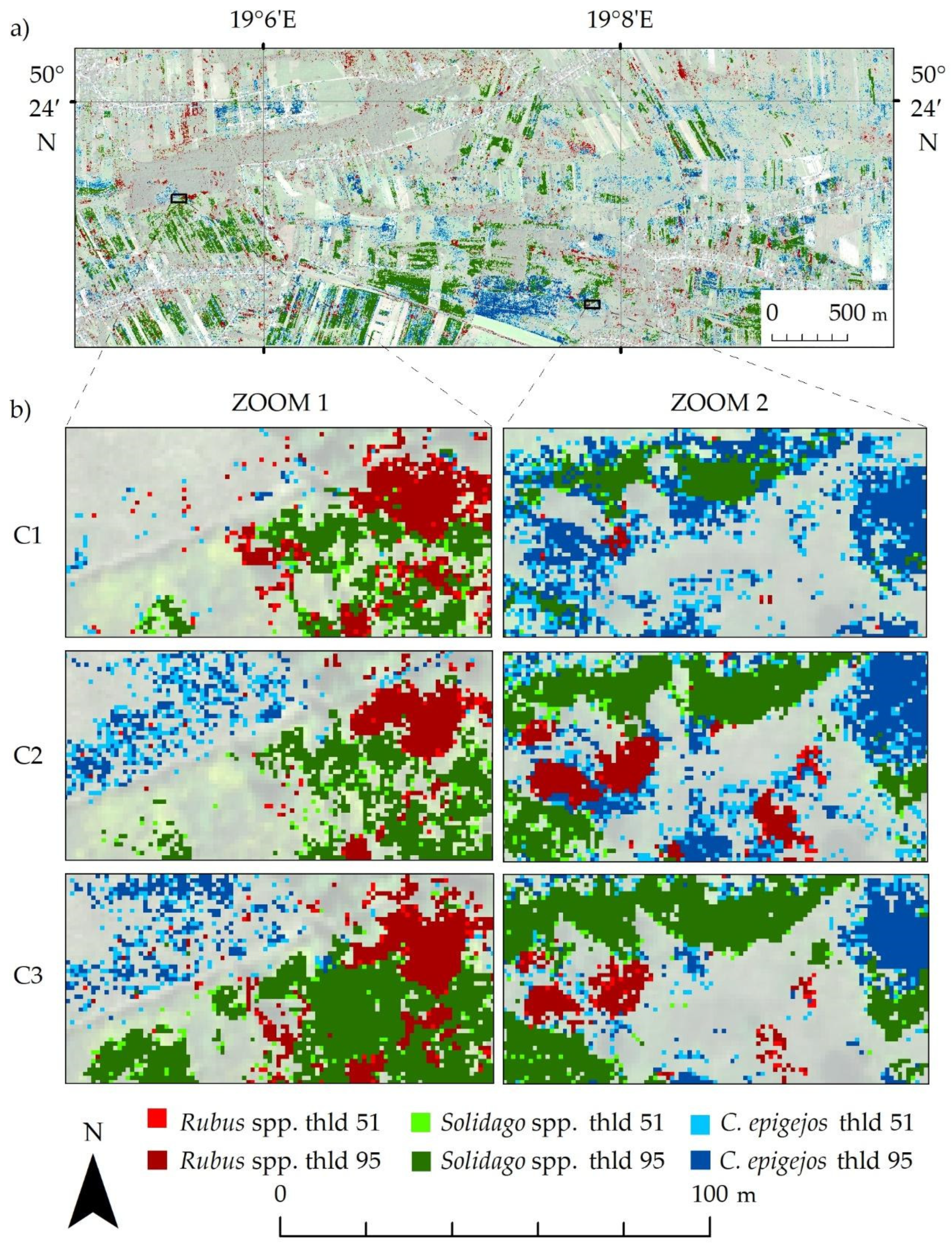
Then, the frequency images were thresholded (thresholds 51 and 95) and combined to obtain a map with classes indicating the presence of a species with lower (
Rubus spp. threshold 51,
Solidago spp. threshold 51 and
Calamagrostis epigejos threshold 51) and higher certainty (
Rubus spp. threshold 95,
Solidago spp. threshold 95 and
Calamagrostis epigejos threshold 95). The figure below shows the obtained thresholding map for campaign 2 (
Figure 8a) and two fragments of the thresholding maps for each campaign (
Figure 8b).
The spatial distribution of invasive and expansive plants identified in the images for three campaigns is similar. The smallest differences between the analyzed campaigns were visible for the Rubus spp. class. This species reproduces mainly by underground rhizomes and stolons, which results in increased compactness and density clumps identified. On the other hand, Calamagrostis epigejos and Solidago spp. spread quickly in the study area through generative and vegetative reproduction. In the first campaign, individual pixels of these species are visible, which in subsequent campaigns grow into large and compact patches identified by the algorithm with greater frequency. Considering the visual analysis of the final maps and statistical accuracy, the best distributions of the analyzed species were obtained in the summer campaign (C2—August). This may result from the flowering period of these plants, which makes it easier to distinguish them from coexisting species.
The area of detected species increases in the following campaigns which is probably related to the development of these plants. The processes of flowering and fruiting as well as the growth of biomass of these plants increase the spectral differences between the identified species and their surroundings. The smallest area is occupied by Rubus spp. (from about 2% of the area in C1 to about 3.5% in C3). Solidago spp. covers from about 5% to 8% of the analyzed area, depending on the date of imaging, but the differences in the area due to the applied thresholds are less than 1 percentage point. In contrast, Calamagrostis epigejos is less recognized by the classification algorithm. The area of the identified species varies depending on the applied threshold—for 51 it ranges from about 3.5% to 4.5%, and for 95 from 6% to 7% of the research area. The differences in the F1-score accuracy for the final maps in individual campaigns are slight. Therefore, it can be assumed that iterative classifications and thresholding of post-classification images in the manner presented allow high accuracy of species identification to be obtained regardless of the date of data acquisition during the growing season. Based on analysis of confusion matrices, background classes were mainly being confused between each other. Similar observations were made for three invasive plant species.
4. Discussion
Having many images presenting different stages of plant development, the problem is to determine the actual range of the studied plants because individual species have different development strategies, e.g., some plants use their resources to produce a large number of seeds, while others produce green biomass or underground rhizomes, which allow them to gain an advantage competitive over the surrounding communities to have better access to the sun, nutrients and water. This means that in the study of invasive and expansive plants, attention should be paid to specific properties of the analyzed species. The second important element is the number of available patterns, which can be used to optimize the classification process and, at the same, correctly assess the quality of the obtained maps [
40]. The optimal solution is to use a large number of patterns (several hundred pixels) that can be used to test different spectral properties of the tested objects in individual iterations of the classification [
41]. In this case, the iteration that offers the best fit for each class can be chosen, and then the main part of the classification can be run [
42]. This situation is difficult in the case of mapping invasive and expansive plants because the spatial patterns created by the studied species and the environment are very variable, depending on local conditions, e.g., agricultural and agrotechnical procedures [
43], as well as land cover, e.g., wasteland [
44,
45]. Classification accuracy for
Rubus spp. (median F1-score around 0.91 for C1, 0.98 for C2, 0.96 for C3) was similar to that reported by other researchers [
46,
47]. Research conducted in Southern Poland using HySpex hyperspectral data and linear discriminant analysis (LDA) achieved median correctness rate 0.91–0.93 for imagery collected in September, 0.95–0.97 for July and 0.97 for June 2016 [
46]. It is worth noting that during summer campaigns LDA was able to better classify
Rubus spp. than in Autumn. In that work, Monte-Carlo-based techniques were mainly used to provide more robust feature selection. Similar conclusions were reported for
Rubus cuneifolius in the eastern parts of South Africa [
48]. Based on Sentinel 2 data and the SVM algorithm, the highest F1-score was achieved in summer (0.58), while scores for datasets acquired in Autumn and Spring were 0.47 and 0.45, respectively. Similarly, high accuracies for
Rubus fruticosus were also achieved using the airborne hyperspectral HyMap data and the mixture tuned matched filtering (MTMF) algorithm during mapping of Kosciuszko National Park (Australia) [
47].
Another work that focused on identification of
Calamagrostis epigejos during the growing season was conducted in Southern Poland near Jaworzno City [
49]; based on HySpex data and the random forest classifier, the authors used 30 MNF transformed bands which resulted in the following F1-scores: 0.64 for June, 0.61 for July and 0.72 for September data acquisition. Lower accuracies might be caused by using referenced data that included reference polygons with relatively low density of
Calamagrostis epigejos (40%). In frame of the same project Kopeć et al. [
20] has shown that minimum density of abovementioned plant species should be no less than 70% in order to be properly identified. Moreover, past research of Sabat-Tomala et al. [
32] has also shown that SVM classifier is more suited for identification of
Calamagrostis epigejos than random forest (SVM F1-score—0.91 and RF F1-score—0.83). Following the same project, but focusing on other geographical areas, identification of
Solidago gigantea was conducted in September 2017 in Lower San River Valley in Poland [
50]. Authors used 30 MNF transformed bands and the random forest classifier, achieving an F1-score 0.73 for
Solidago gigantea. It is worth noting that this research included reference polygons with a density of identified species as low as 20%. Sabat-Tomala et al. [
32] concluded that
Solidago spp. is easily identified on hyperspectral images due to large yellow flowers. F1-score for
Solidago spp. was between 0.96–0.99 depending on the dataset (MNF transformed bands or spectral bands) and classifier (SVM or RF). The same observation was confirmed by Mirik et al. [
51], who achieved higher accuracies when classifying
Carduus nutans for data acquisition conducted while identified plant species were flowering (OA—91% during flowering and 79% before).
Spatial distribution of identified plant species seems to change with data acquisition campaigns (period of plant development), as well as the dataset, e.g., indicators used or classification methods, although these differences oscillate within a few percentage points [
52,
53]. Increase in area covered is most probably caused by vegetation growth, such as increase in height of individual plants, number of leaves and size of them. A set of remote sensing indices for plant species can be implemented in order to capture the characteristics of individual species that become visible in different parts of the growth [
54]. Fast development of invasive species in new habitats and resulting change in spectral properties (during flowering) might be the cause for relative ease when identifying them on the image. Other factors that might change spatial distribution of classified plants are agricultural practices such as moving of meadows or ploughing. Hence it is crucial to properly choose the correct time of year for image acquisition.
F1-scores for analyzed plant species changed by a small fraction when different threshold values were applied (
Table 4). Small changes in F1 do not reflect the quite significant differences in area classified as one of the classified species. For example, on the map obtained for campaign C1 class,
Solidago spp. covers 65.79 ha for threshold value 51, while for threshold value 95 the area covered changes to 56.38 ha, even though both maps have similar F1-score (0.99). A similar effect can be observed for class
Rubus spp., while the largest differences in area cover between maps obtained using different threshold values were observed for class
Calamagrostis epigejos, in which case the difference is almost 100%.
This effect can be caused by spatial distribution of validation polygons and the nature of results obtained using lower threshold values. Part of the reference data is always used for validation. By definition reference data are always located in areas that are covered by a given class, and existence of this class was confirmed during field research. Moreover, while building such a reference dataset, areas that cannot be easily categorized to single class should be actively avoided, e.g., areas covered by a mixture of plant species or areas with low density of specimens belonging to the given class. Reference data can thereby be considered true, and the introduction of mixels into the classifier training or validation dataset can be avoided.
Secondly, using small threshold values almost always results in an increased number of pixels belonging to the given class, which results in larger area cover by the given class on the final map. Choosing the correct (or most useful) threshold value is crucial for application of the algorithm presented in this work. Smaller threshold values deliver maps with areas of potential location of the given class, which can be considered a rough estimation of the real distribution of the class in the image, while higher threshold values deliver maps focused on delivering the most accurate real distribution of class on the image, excluding areas of potential concussion.
5. Conclusions
The method shown in this work allows for the creation of accurate maps from byproducts of iterative accuracy assessment methods. We were able to exploit both synthetic results regarding classification accuracy during the training process (in the form of accuracy measure distribution per class) and post-classification images in order to deliver final maps. One hundred post-classification images were transformed into one map using frequency images and a thresholding approach. Our method ensures that users of iterative accuracy assessment techniques do not have to choose which one of the post-classification images should be considered as the final map. Moreover, it is entirely open to modification and is flexible.
We were able to classify three invasive and expansive plant species with extremely high accuracy. Such results should be treated with caution but prove nonetheless the usefulness of hyperspectral imaging in mapping complex objects. High accuracy of identification may also result from the location of reference polygons in places where species occur with high coverage and density.
It seems that analyzed plant species are mapped more correctly in later campaigns (C3). This is indicated by their increased area cover but might be also an indicator of overestimation. We assume the increased area covered by analyzed plant species is the result of them being easier to identify in later campaigns due to the following reasons: land use (moving), higher stand density, canopy density and flowering and ripening of plants. After analyzing maps obtained in this work (after thresholding and merging of frequency images), we concluded that our method can obtain similar results and is less dependent on date of image acquisition (provided data are collected between June and September).
There is a high degree of uncertainty for some plant species (Calamagrostis) when it comes to spatial distribution of mapped plant species as can be seen on figure showing the relationship between threshold value and the resulting area occupied by class. Such a figure is a valuable source of information previously not available to researchers or map creators.
Threshold values used in this work are nothing more than best guesses and should be considered magic numbers with no significance. Anyone trying to employ this method should use their own judgement when deciding what threshold values should be used in each case.
The use of high-resolution HySpex hyperspectral data (with a spatial resolution of 1 m and 451 spectral bands) allowed to obtain the best results by several percentage points higher than for multispectral data with similar resolution for the same classifiers (RF, SVM). The following steps should be analyzes based on subspace detection or deep learning classifiers, which offer comparable to the used in the studies, because homogenous patterns of the invasive species compactly cover the occupied areas, offering a homogeneous signal, especially during the flowering period, when they are covered with yellow perianth. An identification of invasion bridgeheads remains a problem, as individual plants enter heterogeneous polygons creating mixes of spectral signals.


