Article

Distribution and Evolution of Supraglacial Lakes in Greenland during the 2016–2018 Melt Seasons

1
School of Geography and Planning, Sun Yat-sen University, Guangzhou 510060, China
2
School of Geospatial Engineering and Science, Sun Yat-sen University, Southern Marine Science and Engineering Guangdong Laboratory (Zhuhai), Zhuhai 519000, China
3
Department of Geography, Texas A&M University, College Station, TX 77843, USA
*
Author to whom correspondence should be addressed.
Remote Sens. 2022, 14(1), 55; https://doi.org/10.3390/rs14010055
Submission received: 24 November 2021 / Revised: 15 December 2021 / Accepted: 20 December 2021 / Published: 23 December 2021
(This article belongs to the Special Issue Remote Sensing of Environmental Changes in Cold Regions Ⅱ)

Abstract

:
In recent decades, the melting of the Greenland Ice Sheet (GrIS) has become one of the major causes of global sea-level rise. Supraglacial lakes (SGLs) are typical hydrological features produced on the surface of the GrIS during the melt seasons. The existence and evolution of SGLs play an important role in the melting process of the ice sheet surface. To understand the distribution and recent changes of SGLs in Greenland, this study developed a random forest (RF) algorithm incorporating the texture and morphological features to automatically identify SGLs based on the Google Earth Engine (GEE) platform. Sentinel-2 imagery was used to map the SGLs inventory in Greenland during the 2016–2018 melt seasons and to explore the spatial and temporal variability characteristics of SGLs. Our results show changes in SGLs from 2016 to 2018, with the total area decreasing by ~1152.22 km2 and the number increasing by 1134; SGLs are mainly distributed in western Greenland (SW, CW, NW) and northeastern Greenland (NE), where the NE region has the largest number of observed SGLs and the largest SGL was with the surface area of 16.60 km2 (2016). SGLs were found to be most active in the area with the elevation of 800–1600 m and the slope of 0–5°, and showed a phenomenon of retreating to lower elevation areas and developing to steeper slope areas. Our work provided a method for rapid inventory of SGLs. This study will help monitor the mass balance of the GrIS and predict future rapid ice loss from Greenland.

1. Introduction

In recent decades, the Greenland Ice Sheet (GrIS) has been in a state of accelerated mass loss and has become a major contributor to global sea-level rise [1,2]. Since 1990, the surface melting and runoff of the GrIS have increased due to global warming [3]. According to the GRACE observations, a total of about 3902 ± 3420 Gt of GrIS mass was lost between 1992 and 2018, of which the proportion of ice sheet surface melt contributed to about 50.3% of the GrIS mass loss, resulting in a mean sea-level rise of about 10.8 ± 0.9 mm [2]. Currently, ice sheet surface ablation becomes one of the main causes of GrIS mass loss and even global sea-level rise.
The GrIS produces a large amount of meltwater during the melt seasons, which is transported on the surface of the ice sheet by topography and other factors [4]. Part of the meltwater collects in topographic depressions on the ice cap surface through surface runoff, forming supraglacial lakes (SGLs) [5]. SGLs tend to form at the same location each year due to the control of basal topography depressions of the Greenland ablation zone [6,7]. Thus, SGL is a typical annual hydrological feature of the GrIS during the melting season. The formation and evolution of SGLs can affect the mass balance and dynamics of the GrIS [6]. On the one hand, the presence of SGLs creates positive feedback on ice sheet surface ablation due to their low albedo; on the other hand, SGLs act as transient storage buffers for meltwater runoff, and their intermittent filling and draining establish a link between the ice sheet surface and the subglacial hydrological system, thus affecting ice dynamics [8,9].
Considering the limitations of traditional in situ observations, remote sensing technology has played a better role in tracking and monitoring the spatial and temporal changes of SGLs on a large scale and systematically [10]. MODIS images with high revisit frequency over a wide area are now widely used in the monitoring of SGLs for long time series. Leeson et al. [11] used MODIS imagery to investigate the distribution and interannual variability of SGLs in the Russell Glacier region of the western GrIS in 2005–2007. Sundal et al. [12] studied the seasonal evolution of SGLs in three regions (southwest, northwest, and northeast) of Greenland using a total of 268 MODIS images collected in 2003 and 2005–2007. However, MODIS imagery shows limited capability to identify small lakes (<0.125 km2) and difficulty providing detailed information, due to its low spatial resolution [13,14]. In recent years, high spatial resolution remote sensing images represented by Landsat 8, Sentinel-2, etc, have been used often in the studies of SGLs [15,16,17]. Williamson et al. [13] combined Landsat 8 and Sentinel-2 imagery to monitor the evolution of SGLs in western Greenland from May to October of 2016, and found that the average area of the lakes using data from Landsat 8 was nearly 50 times lower than the area measured using MODIS imagery [14]. Despite the Landsat 8 data showing the potential of detecting and mapping SGLs on the GrIS, Sentinel-2 data with high spatial resolution (10 m) provides new opportunities for the automatic mapping of SGLs [18]. The previously mentioned work by Williamson et al. [13] shows that Sentinel-2 imagery (10 m) is superior in identifying small lakes (<0.125 km2) to MODIS imagery (250 m). Shugar et al. [19] used 254,795 Landsat images from Google Earth Engine (GEE) to map global glacial lakes between 1990 and 2018. The study shows that the GEE platform has the ability to rapidly map glacial lakes on a large scale based on a long time series of optical remote sensing data. The authors propose that the GEE platform, combined with higher resolution imagery (e.g., Sentinel-2) could improve the ability to identify smaller lakes and could be applied to the analysis of glacial lakes on a larger scale.
At present, the methods for extracting SGLs based on optical remote sensing images can be mainly categorized into two types: threshold methods and classification methods. The threshold method based on water body indices (such as NDWI, MNDWI, etc.) is a fast and effective semi-automatic extraction method [20]. Stokes et al. [21] and Bell et al. [22] automatically identified and mapped the distribution of SGLs on the Antarctic ice cap based on NDWI and NDWIice (red/blue band) thresholds, respectively. However, the threshold method lacks transferability due to the influence of different background environments [19]. Box and Ski et al. [23] developed a single threshold to differentiate between meltwater and ice using the MODIS reflectance ratio based on bands 1–3. However, the method does not perform well in the identification of certain types of lakes, such as deep lakes [24]. Ouma et al. [25] concluded that the threshold method relying only on the water body index (NDWI) has some shortcomings in the identification of lake boundaries. In recent years, machine learning algorithms (e.g., RF, SVM, etc.) with advantages in terms of great stability, high classification accuracy, and fast computing speed has been proven successful in ice-water classification [26]. Xie et al. [27] tested three machine learning algorithms, SVM, RF, and CART, to extract supraglacial debris and concluded that RF outperformed other models (RF had an overall accuracy of 96%, a 6% improvement over SVM). Wu et al. [28] compared four machine learning classifiers (MLR, SVM, RF and GBT) for mapping lake ice cover. The results demonstrated the RF classification with the strongest spatial transferability over 17 lakes has the potential to mapping lake ice cover globally. Dirscherl et al. [18] combined the RF algorithm with 12 variables to map Antarctic SGLs with an average accuracy of 86%, and found that RF combined with an optimal feature assembly allows for the good spatio-temporal transferability of spatially independent regions. These studies prompted us to explore the identification of SGLs using RF due to its capacity for feature learning and algorithm running efficiency [29,30].
Although SGLs are widely distributed within the ablation zone of the GrIS, lake investigations have so far been limited to the southwest and northeast [31,32,33]. To investigate the impact of supraglacial meltwater accumulation on Greenland ice dynamics and mass balance in more detail, comprehensive mapping of Greenland SGLs is needed. However, because the SGLs on the GrIS are generally small and unstable, tracing their variation is limited by significant amount of manual interpretation and editing [10,34]. The GEE platform, which has open and dense Sentinel-2 archive data, offers the advantage of fast batch data processing for large study areas [10,35].
In this study, our objectives are:
(1)
To present an automatic Machine Learning (ML) method for identifying the SGLs on the GrIS and mapping their spatial-temporal distribution using the Sentinel-2 imagery based on GEE.
(2)
To monitor the characteristics and dynamic evolution of SGLs on the GrIS during the 2016–2018 melt seasons.

2. Study Area

The study area was the entire Greenland region which is known as the largest island in the world with a highest elevation of ~3700 m and an estimated area of ~2.20 million km2 [36,37] (Figure 1). The GrIS is the second-largest continental ice sheet in the world after the Antarctic ice sheet, with an area of 183.39 × 10⁴ km2 and an average ice thickness of 2300 m [38,39]. SGLs form annually and are widely distributed within the GrIS ablation zone which is a typical area to study the dynamic evolution of SGLs [40].
This study uses the regional boundaries defined in the Greenland watershed and ice sheet produced by E. Rignot and J. Mouginot and used by IMBIE 2016; thus Greenland was divided into six regions: NO, NW, NE, CW, SW, and SE [39].

3. Data and Methods

In this study, we implemented the rapid extraction of SGLs contours and analyzed the annual variation of SGLs across entire Greenland during the 2016–2018 melt seasons based on the GEE platform. The workflow, shown as Figure 2, comprises four main steps: (1) select suitable images to form the initial dataset according to the seasonal melting period of the GrIS; (2) use the RF algorithm to classify the images by combining the ice-water’s spectral (Normalized Difference Water Index adapted for ice, NDWIice) and texture features (Gray-Level Co-occurrence Matrix, GLCM); (3) filter out the water spots caused by classification errors and extract the SGLs boundaries by a morphological algorithm; (4) verify the accuracy of the extraction results, produce the SGLs dataset and analyze the spatial and temporal evolution of SGLs.

3.1. Image Pre-Processing

This study used Sentinel-2 imagery from the GEE database for the 2016–2018 Greenland melt seasons (1 May to 30 September). The Sentinel-2 Level-1C imagery products used in this study were atmospherically and geometrically corrected [42]. The Sentinel-2 imagery covers a total of 13 wavelength bands including visible, near-infrared, and short-wave infrared ranges, with a spatial resolution of up to 10 m [43]. Based on the reflectance range of the water bodies, this study used B1-B8 to represent the spectral characteristics of the water bodies. The images of entire Greenland area were chunked to improve the spatial and temporal efficiency of the image processing algorithm. Firstly, the cloud pixels are removed according to the QA60 band of the image to exclude the influence on the water identification; then Greenland was divided into 100 × 100 sub-regions according to the Fishnet created by ArcGIS10.5; finally, the average value of the melt season images of the sub-regions was calculated separately to synthesize an annual ablation period image.

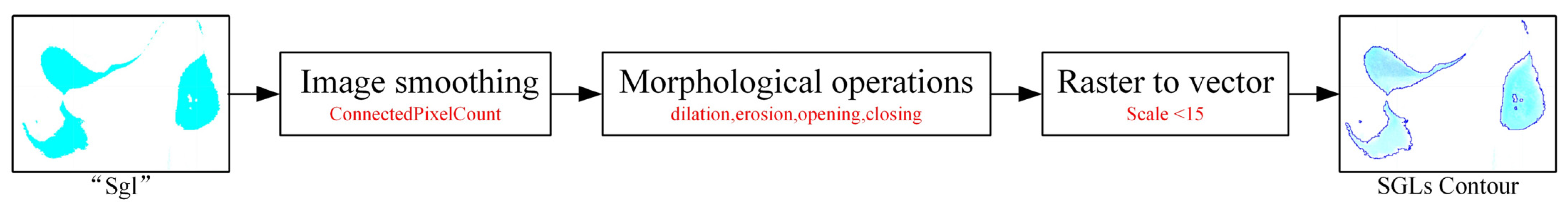
3.2. Automatic Identification of SGLs

Automatic identification of SGLs based on the GEE platform was mainly divided into three parts: sample point generation, image classification, and post-classification processing. This study created two types of training samples, “Sgl” and “Not sgl”, where “Sgl” represents SGLs, and “Not sgl” represents different types of features other than SGLs, such as ice, rocks, glacial runoff, etc. The sample points (about 15–20) were created and evenly distributed within each sub-region (~215 km2). Two conditions needed to be satisfied for the online selection of sample points: (1) SGLs can be observed within the corresponding sub-regions. Since SGLs are distributed near the edge of the meltwater ice sheet, some inland and center regions with no observed SGLs were excluded from this study. Therefore, a total of about 10,000 sample points within about 500 sub-regions were available each year. (2) The correction of the sample points was proved based on visual checking by overlaying Sentinel-2(10 m). Due to the efficiency limitation of zooming in on images in the GEE, the sample points were exported to KML format and then imported into the Google Earth platform. The correctness of the sample points was checked visually by overlaying contemporaneous high-definition base maps. The sample points that met the selection criteria are used as the training data set for image classification.
A suitable combination of feature variables can effectively improve computational efficiency and classification accuracy [44,45]. First, according to the reflection characteristics of water, ice, and rocks, the NDWI index can be used for the classification of open surface water [18]. Since the reflectance of the blue band is relatively high in a glacial environment, the normalized water body index NDWI ice = (BLUE-RED)/(BLUE+RED) can better identify the ice waterbody features than NDWI(GREEN-NIR/GREEN+NIR) [46]. Secondly, since ice and water may have similar backscatter signatures within the scene, mixed reflections can appear at the junction of water and ice, leading to confusion in the extraction of the edge of the lake [21]. The use of GLCM to determine texture features can effectively improve the classification results [26]. The four most commonly used feature variables, including Contrast (contrast), Sum Average (savg), Angular Second Moment (asm), Entropy (ent) were used in this work. Finally, we input the NDWI ice and GLCM features into RF model to identify the pixels of the SGLs.
Three concerns need to be considered to extract the contours of SGLs after image classification: (1) waters with spectral features similar to SGLs, resulting in misclassification of water spots; (2) “Sgl” classes obtained after classification often contained SGLs and narrow runoff; (3) output scale affects the degree of SGL boundary extraction (“too large” or “missing”), due to the computational limitations of the GEE platform. The flow chart shown as Figure 3 illustrates how these problems have been solved. First, the image was smoothed and applied with the ConnectedPixelCount function to eliminate less than 10 pixels (~1 × 10⁻⁴ km2) of the “Sgl” class; then, we conducted opening operations based on small rectangle structural elements to remove isolated water points around water patches to form a complete, well-fitted lake contour; finally, the SGL vector boundary was extracted, and the scale of the transformed polygon was set to less than 15. Any independent elongated rivers could be manually eliminated later.

3.3. Production and Validation of the SGLs Dataset

There were two goals of mapping the SGLs dataset in this study: (1) to investigate whether there exists any SGLs on GrIS smaller than 0.18 km2 documented by previous research [14,47]. This minimum SGL size (~0.18 km2) was computed based on MODIS pixels (250 m). Our other goal was to (2) ensure the extracted lake vector boundaries deviated from the Sentinel-2 (10 m) images by no more than 2 pixels. Since the whole area of Greenland is vast, the boundary extraction scale of the SGLs vectors was not fully applicable to some sub-regions where small SGLs (≤0.02 km2) are sparsely distributed, due to the computational limitation of GEE. Therefore, the combined SGLs vector dataset was overlaid with the contemporaneous Sentinel-2 remote sensing images for visual verification of the SGL datasets for Greenland in 2016, 2017, and 2018 melt seasons.
Considering the uneven distribution of SGLs throughout Greenland, a buffer zone was established at 1.5 times the average annual area of the SGLs. About 2500 sample points per year were randomly selected on the buffer zone to construct the validation sample dataset. Four accuracy assessment metrics were calculated based on the confusion matrix: overall accuracy (OA), producer accuracy (PA), user accuracy (UA), and kappa coefficient (K) (Table 1).
The calculation formula for each precision indicator (OA, PA, UA, K) was as follows:
O A = T P + T N N
P A = T P T P + F N
U A = T P T P + F P
K = O A P e 1 P e
P e = ( T P + F N ) ( T P + F P ) + ( F P + T N ) ( F N + T N ) N 2

4. Results

4.1. Accuracy Assessment of SGLs Extraction

Figure 4 shows the SGL extraction results for detailed sub-regions according to the geographical subdivisions. Since some runoffs with large amounts of water were connected with SGLs as an inseparable whole, they were included in the final results of SGL extraction. These clearly show that the proposed method can identify the SGLs contours from the Sentinel-2 images well.
The overall classification accuracy of the SGLs in Greenland during the 2016–2018 melt seasons was evaluated based on the validation sample dataset (as shown in Table 2). All four accuracy metrics were above 0.94, indicating that the method used in this study achieved accurate extraction of the SGL contours.

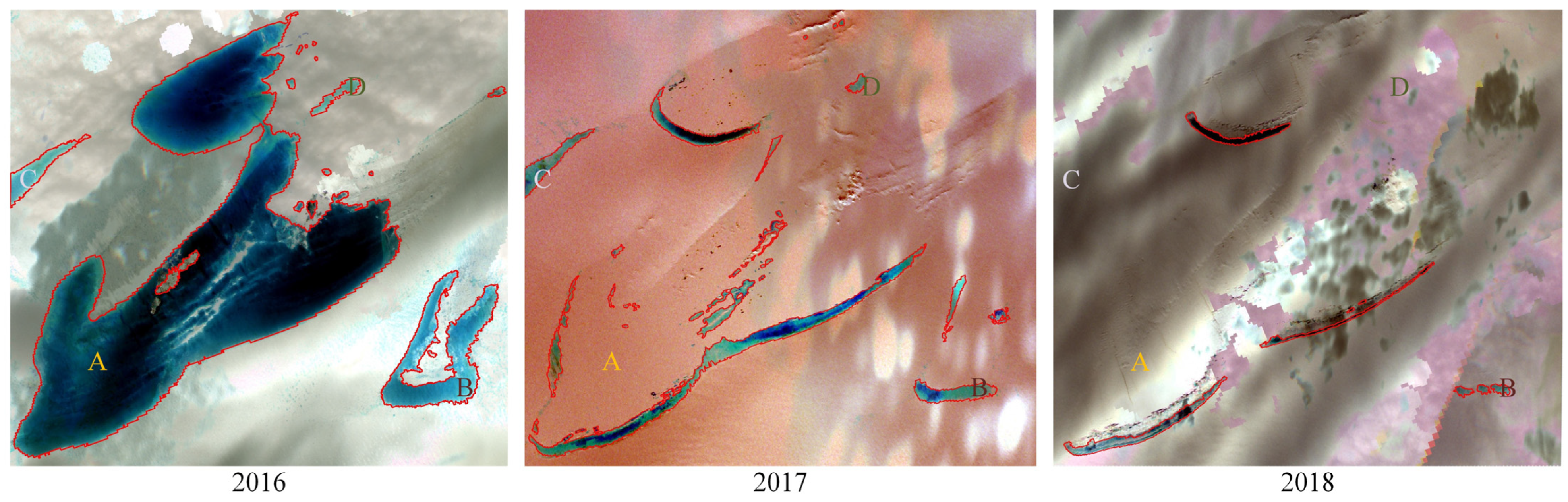
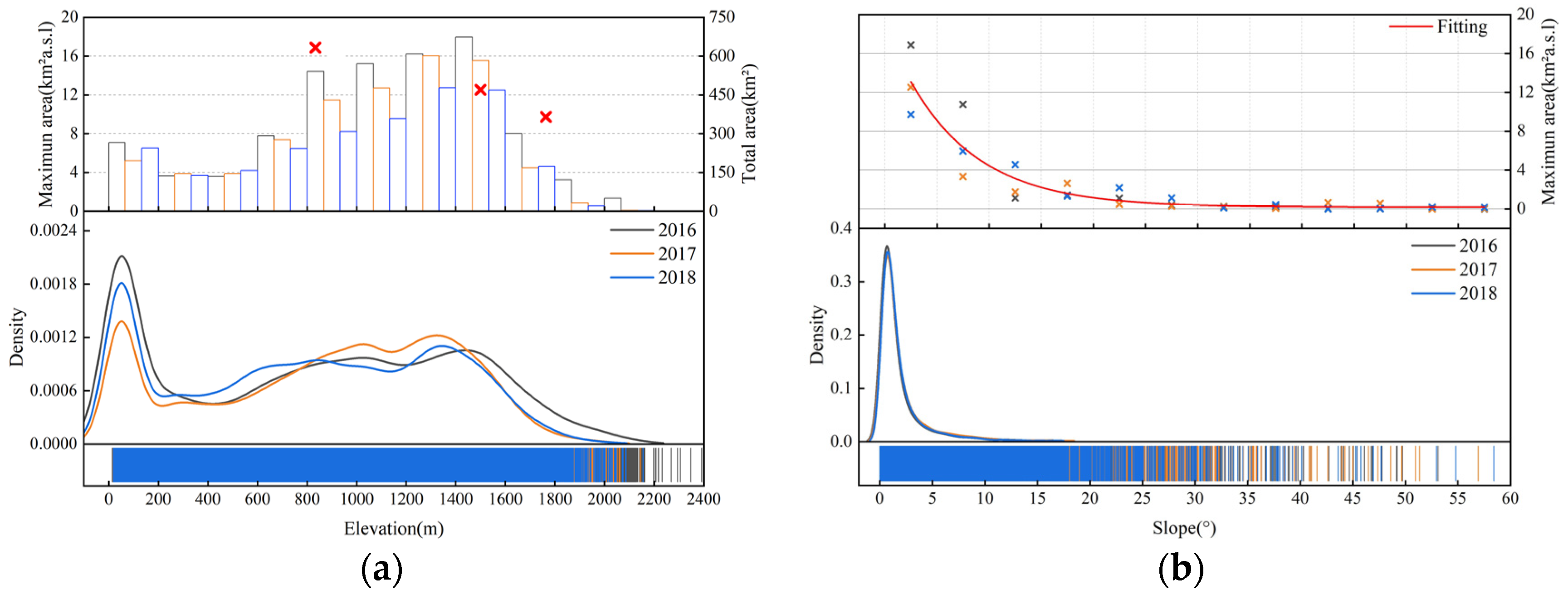
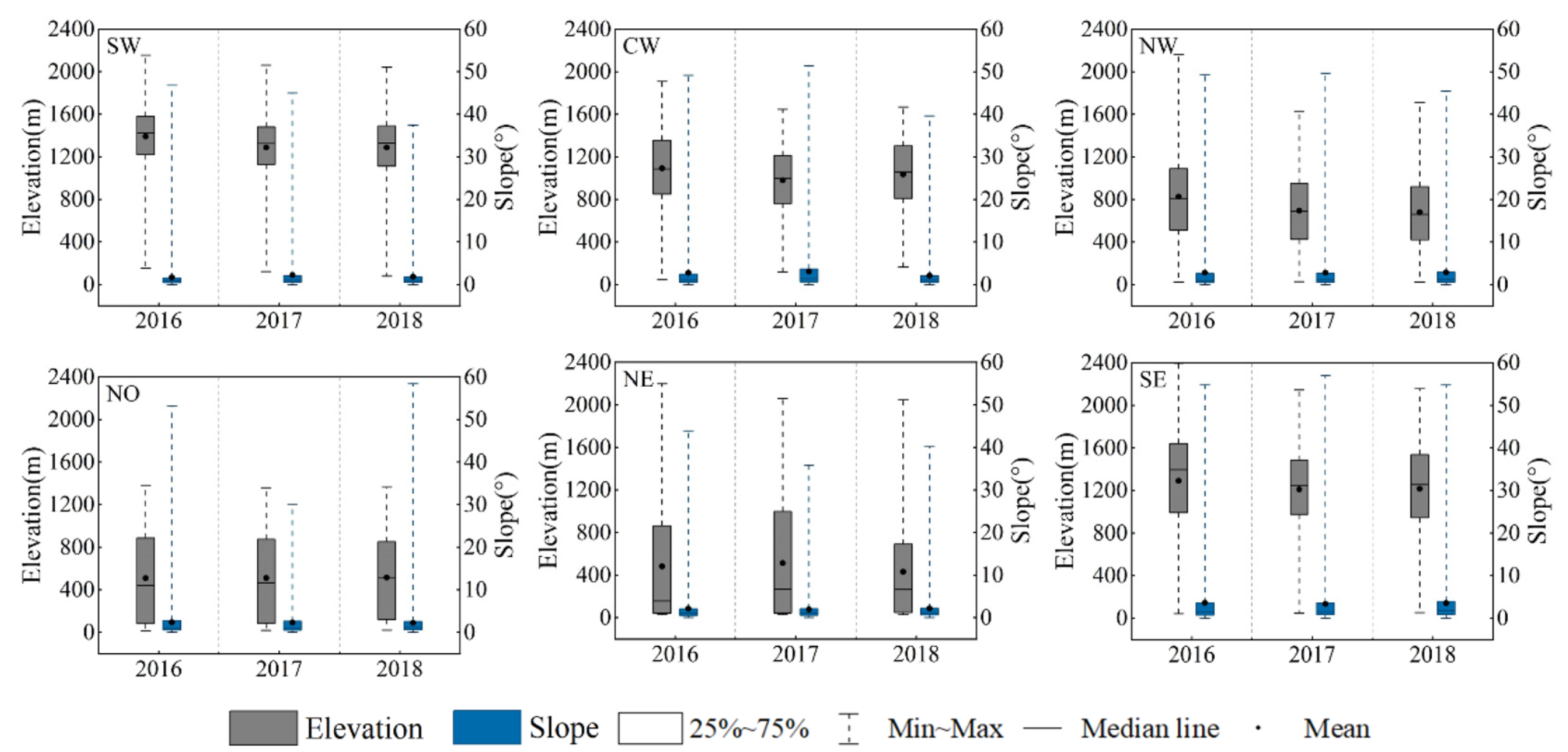
4.2. Spatial Distribution of SGLs

We mapped 23,389, 24,065, and 24,523 SGLs in Greenland with a total area of approximately 3751.18 km2, 3059.21 km2, and 2598.96 km2 during the 2016–2018 melt seasons, respectively. The recorded sizes of the individual ranged from 0.0002 km2 to 16.60 km2. The SGLs were divided into five categories according to individual lake size: 0–0.5 km2, 0.5–1 km2, 1–5 km2, 5–10 km2, 10–20 km2. Figure 5 shows the spatial and temporal distribution of SGLs for five categories.
The total number of small lakes (0–0.5 km2) accounted for over 90% of the total lakes in each year during 2016–2018, and increased from 21644 (2016) to 23365 (2018). The number of other type lakes (≥0.5 km2) changes in the opposite direction were insignificant. Thus, the year-to-year change in the total number of SGLs was dominated by small lakes (0–0.5 km2). Medium and large lakes (0.5–20 km2) were mainly found in the SW and NE regions during 2016–2018, however, they gradually disappeared within two years, and no large lakes (10–20 km2) were found in 2018. Figure 6 shows the evolution of the largest lake observed in 2016 which was gradually split into multiple smaller lakes and subsequently largely disappeared. This may explain the increase in small lakes and the decrease in large lakes between 2016–2018. The split of large lakes can be the main contributor to the increase of small lakes.
We calculated the elevation and slope of the SGLs by the ArcticDEM (2 m) [48]. Figure 7 shows that the SGLs in the study area were found at an altitude of <2400 m and a slope of <60° from 2016-2018. The distribution density of SGLs in different elevation and slope ranges shows that the maximum elevation of lakes occurred in 2016 and the highest slope was reached in 2018. Figure 7a shows that while a large number of lakes were found in the elevation range of 0–200 m, the total lake area was relatively small, and medium and large lakes were mainly observed in the elevation range of 800–1600 m. The annual maximum lake area became smaller with increasing elevation. Figure 7b shows that SGLs were mainly distributed in the slope range of 0–5°, and the lake area gradually became smaller with increasing slope. In summary, it was found that the annual disappearance of large lakes and the vigorous development of small lakes led to a phenomenon of SGLs in Greenland retreating to lower elevations and steep slope areas during 2016–2018.

4.3. The Dynamic Changes of SGLs

We calculated the inter-annual rate of change in terms of the total area and the number of SGLs in different regions (Figure 8 and Table 3) to analyze the temporal and spatial distribution and the dynamic changes of SGLs in the study area from 2016 to 2018. As shown in Figure 8, the total area of SGLs counted in the SW region was the largest in each year, followed by NE, CW, and NW, NO, and SE regions. The total quantity of SGLs in the NE region was the largest in 2016 and 2018, followed by SW, NW, CW, NO, and SE, in order. In summary, SW and NE were the regions with the largest total area and number, respectively. Considering the total area and quantity, SGLs were more concentrated in western (SW, CW, NW) and NE Greenland. It is worth noting that small lakes (0-5 km2) were the main contributors to the quantity found in the NE region (about more than 95%), and were mainly clustered near the northeast corner of Greenland.
We observed general changes of a decreasing area and increasing number of SGLs in the study area from 2016–2018 (as shown in Table 3). The lake area decreased, shrinking by ~642.9 km2 (~17%) in 2016–2017, slightly slowing down to ~458.78 km2 (~15%) in 2017-2018. The increasing number of lakes was not obvious, increasing by only ~689 (~3%) in 2016–2017 and 475 (~2%) in 2017–2018, respectively. Spatially, the largest changes to the lake area and number in 2016–2017 occurred in the NW (~38%) and SW (~52%) regions, respectively, and the smallest changes occurred in the SE (~4.9%) and NO (~0.4%) regions, respectively. The largest changes to the lake area and number in 2017–2018 occurred in the NW (~24%) and NE (~44%), and the smallest changes occurred in the CW (~1.8%) and SE (~8.4%) regions, respectively. Interestingly, the changes in the area and the number of SGLs in each region were also inconsistent. Each region of Greenland has certain special characteristics that lead to important differences in the response mechanisms of the GrIS to climate at the local and regional scale [49]. The GrIS–atmosphere feedback affects the variation of ice sheet thickness and ice flow, which are the important factors determining the formation and evolution of SGLs [50]. Only the area and number of ice-surface lakes in the SW and SE regions increased in 2016–2017 and 2017–2018; the area and number of SGLs in the NW and NO regions were continuously decreasing year by year. (Table 3). This reflects the opposite changes of SGLs in the SW and NO regions on the same time scale.
In summary, it is shown that SW, NW, and NE were regions with more medium and large lakes (0.5–20 km2), to the extent that they were the dominated the variation to SGLs in the whole study area, and the variation of the CW, NO and SE regions, with mainly small and medium-sized lakes (0–10 km2), was relatively stable. Combined with the interannual variation of lake types in each region (Figure 5), medium and large lakes that dominate the interannual variation of total area evolved into small lakes or even disappeared during drainage or refreezing, which is compensated by newly formed small-sized lakes with an average annual raise of 1%, resulting in opposite trends in the area and number of SGLs in the study area. The extent of changes in large and small lakes determined the changes in the area and number of lakes in different regions, and the lakes in each region determined the overall evolution of SGLs in the study area in the process.
The elevation and slope distribution of SGLs in each region from 2016–2018 (Figure 9) showed that the highest elevation occurred in the SE region in 2016 and the steepest slope occurred in the NO region in 2018. The average elevation of SGLs in the southern region (SW, SE) was higher than that in the north (NW, NO, NE). Of these, the SW region not only had the largest area of SGLs, but also has the highest average elevation of SGLs. The southern region (SW, SE) was observed to increase in area and number of SGLs when other regions saw significant decreases in SGLs. This indicates that SGLs tend to develop at higher elevations; the phenomenon of SGLs retreating to lower elevations and lower slopes was observed in all regions from 2016 to 2018, however, the new formation of small lakes in the NO region in 2018 exposed the possibility of SGLs developing towards steeper slopes.

5. Discussion

5.1. Comparing with Previous Studies on SGLs Evolution

To date, studies of SGLs in Greenland have focused on the southwest and northeast and were mostly focused on determining lake depth and volume. We focused on studying the spatial and temporal distribution and interannual variability of SGLs. Due to the lack of a free and available inventory of SGLs for the entirety of Greenland, we only compared related studies of local areas. A comparison of the quantitative descriptive information of SGL evolution from 2016 to 2018 is presented in Table 4. As the study areas for comparison were not identical, the areas and numbers of SGLs are not comparable. Therefore, we only performed our comparison and discussion from the perspective of interannual trends of lake area and number. The changes in the area and number of SGLs in the CW and NE regions from 2016–2018 obtained from our monitoring were generally consistent with the conclusions drawn by Yuan et al. [31] and Philipp et al. [51] respectively. This level of consistency shows that the automatic ML method of combining ice-water spectra and texture features was feasible for monitoring SGLs using Sentinel-2 imagery.
However, we found differences in the area and number changes of SGLs in the CW and NE regions among the two comparison studies in 2017 and 2018, respectively. This may be attributable to the use of different resolutions in the remotely sensed data and inconsistent study areas. Yuan et al. selected a local area in southwestern Greenland to extract SGLs from Landsat 8 (30 m) imagery. We believe that the SGLs mapped by Sentinel-2 (10 m) imagery with higher resolution were more consistent with the validation data. Therefore, more detailed information will be acquired to compare with the work of Yuan et al. using lower resolution imagery. Philipp et al. used Sentinel-2 imagery to extract SGLs from the 79°N glacier area in northeast Greenland and reported that the number of SGLs decreased from 477 to 288 in 2016–2018. The NE region saw the most significant increase in the number of SGLs from 2017–2018. Based on the inventory of SGLs we surveyed, there was a significant decrease in medium lakes (0.5–5 km2) near the grounding line of the NE region and a more extensive development of small lakes (0–0.5 km2) in its NE corner (80°N–81°N) in 2018. As the study by Philipp et al. did not include the NE corner, they were only able to monitor a reduction in the number of lakes due to the decline in medium lakes. To some extent, our results support their conclusion because their comparison study areas were all included in the scope of this study.
Moreover, we monitored the presence of many small lakes in the NE corner which account for approximately 26% of the total number of SGLs in the NE region each year between 2016 and 2018. The current studies of SGLs in NE Greenland mainly focused on the vicinity of the glacier at 79°N, and it is easy to overlook the great potential of the NE corner to harbor SGLs.

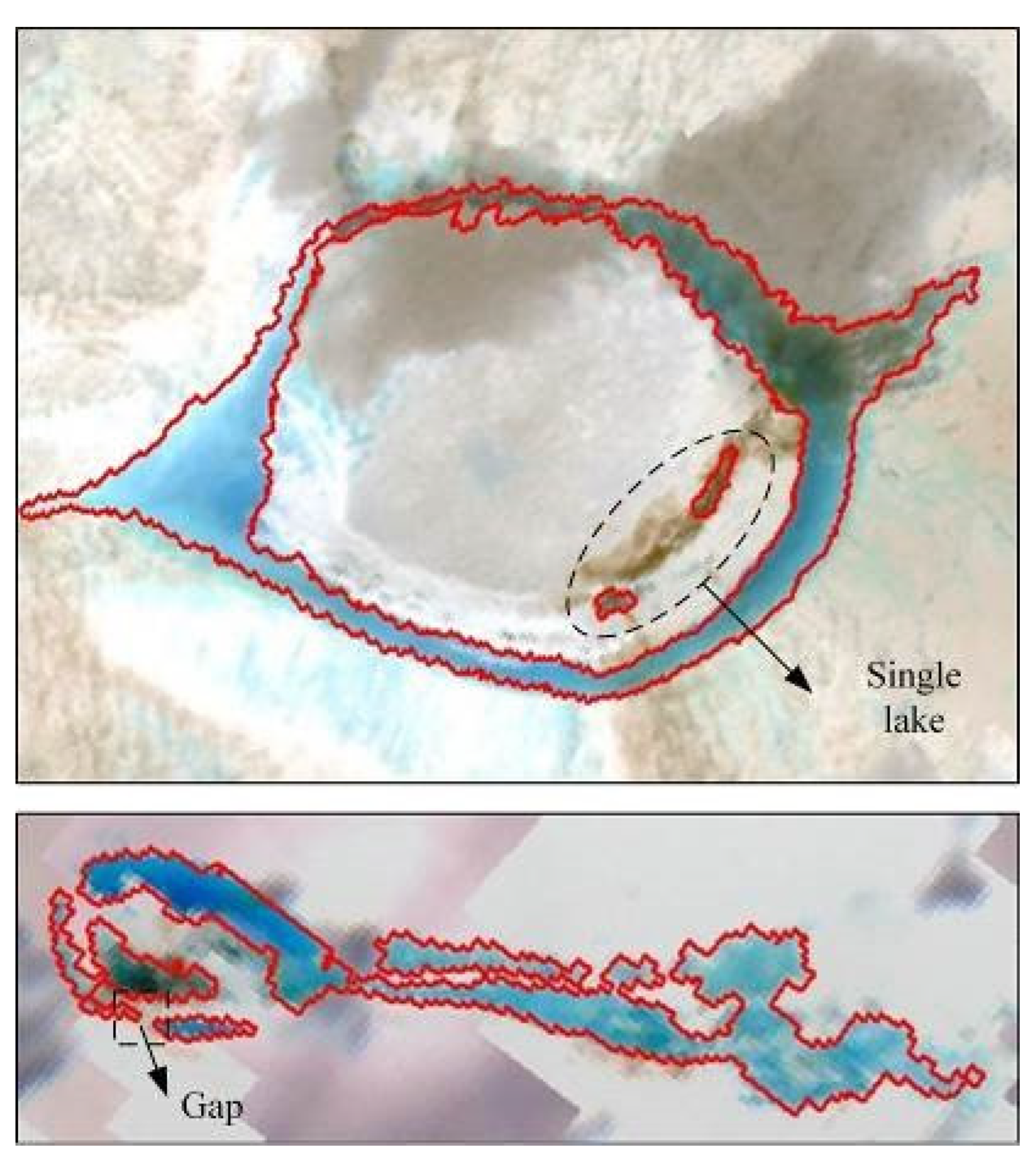
5.2. Uncertainties of SGLs

The uncertainty in contouring SGLs and determining the number of lakes mainly comes from the computational limitations of the GEE platform to automate the extraction of lake vector boundaries. The large variations in the size of individual lakes (0.0002 km2–16.60 km2) leads to the inability of GEE to determine the appropriate scale for uniform output in the process of extracting lake boundaries. To ensure most of the lake contours were extracted completely, the very small lakes (<0.018 km2) were ignored, resulting in the total area and number of these very small lakes being underestimated. As SGLs tend to split during drainage or refreezing and are not necessarily complete individuals (Figure 10), an increase in the number of vectors identified was observed. In the process of producing the SGL dataset, we added missing lakes by the manual digitization and merging of fragmented vectors (defined as a complete “SGL”) against the actual images.
The minimum detectable size of SGLs derived from Sentinel-2 data (10 m) was 0.0002 km2 in this study, which is nearly 100 times lower than the error associated with William et al. [14,43] using MODIS (250 m). This means that our SGL dataset contains lakes that are smaller than the smallest SGL size (~0.18 km2) in the current record.
We report uncertainty in lake sizes and numbers, especially for the incomplete lakes. The computational memory of the GEE platform limits the minimum scale of the extraction of lake contours, which leads to increased uncertainty. We applied manual corrections and visual checks to ensure that the extracted lake profiles followed the actual lake boundaries to ensure the integrity of the full-area extraction.

5.3. Implications of Climatic Conditions

The formation and evolution of SGLs are controlled by climate change [52]. Accelerated Arctic warming over recent decades has led to increased melting of the GrIS, thus providing the conditions to promote SGLs development [53]. 2016 was the record-breaking melt year since records began, and the largest size of a single SGL (16.60 km2, in our three-year record) occurred during this melt season [54]. However, during the summers of 2017 and 2018, Greenland experienced strong cyclonic circulation that resulted in the southward transport of cold air from western Greenland, and Hurricane Nicole brought heavy snow and rain to eastern Greenland [55,56,57]. The GRACE-FO satellite monitored a slowdown in GrIS melting in 2017 and 2018 compared to 2003–2016 [47]. We observed a significant decrease in the total area of SGLs in 2017 and 2018 compared to 2016. SGLs are sensitive to climatic conditions and still form in the lower part of glaciers even in cool years [58,59]. This could also explain the fact that, in the context of the slowdown of GrIS melting, the climate change sensitive SW and the NE region with two large glaciers (ZI and 79°N) still developed many new small lakes in 2017 and 2018, directly affecting the overall change to in the number of SGLs [60,61]. Measurements at 20 weather stations of the DMI (Danish Meteorological Institute) indicated that the temperatures were markedly lower (up to 3 °C) in 2017 (March–July) than in August of 2016 in coastal northeast and western Greenland [62,63]. Cold summer temperatures slowed the melting of the ice sheet, leading to significant dynamic changes in the SGLs of western (SW, NW) and eastern (NE) Greenland. Heavy snowfall in eastern Greenland covered the SGLs on the ice sheet and delayed the formation of new SGLs, limiting the formation of large lakes [47]. As a result, the large lakes in the NE region gradually disappeared in 2017 and 2018 and were followed by more small lakes. The SGLs in each region formed significant feedbacks to climate change and showed different changes in lake areas and numbers. The quantification of the impact of climate change (various meteorological factors) on the evolution of SGLs in different regions of Greenland needs further study.

6. Conclusions

We have presented a Sentinel-2 imagery based inter-year investigation during the melt seasons of SGLs on the GrIS in this work. The SGLs of Greenland during the 2016–2018 melt seasons were extracted and the dynamic characteristics of SGLs over 3 years were analyzed. RF combined with the texture features and morphological algorithms based on the GEE platform enabled us to extract SGLs automatically and effectively in this study area with an accuracy of over 94%, which was verified by 2500 sample points every year. Future work is needed to analyze a long-term time series of SGL evolution.
Our results have calculated that the total area of SGLs in 2016 was 3751.18 km2, and that this area has subsequently beendecreasing, reaching a low point of 2598.96 km2 in 2018. The total number and area changed in opposite directions, such that 24523 SGLs were observed in 2018, which was the highest number of the three years. The largest individual lake appeared in 2016, then it gradually shrunk while forming some smaller lakes, until it disappeared in 2018. The loss of large lakes and the formation of new small lakes caused a decrease in the total area and an increase in the total number of SGLs from 2016 to 2018.
Regionally, SGLs are mainly clustered in western (SW, CW, NW) and northeast Greenland. The NE region not only has the largest lake but also nurtures many small lakes, especially near the NE corner. There were differences in the evolution of SGLs at the regional scale. The disappearing SGLs were mainly located in the NW, SW, NE regions, and there were a few new SGLs in the SE region and the NE corner. Considering the topographic variations, we found that SGLs were most active in the areas with an elevation of 800–1600 m and a slope of 0–5°. Large lakes tend to develop more at higher altitudes and lower slopes. The significant decline in large lakes and the continued growth of small lakes from 2016–2018 resulted in more SGLs appearing at lower elevations and higher slopes in 2018 than in the other years. The average elevation of SGLs in southwest Greenland was higher than in other regions, creating good conditions for the development of medium and large lakes.
In addition, we found that the evolution of SGLs had a positive response to climate change. SGLs disappeared significantly in the northeast and western Greenland, which experienced unusually cold summers in 2017 and 2018. Applying the annual inventory of the SGLs we investigated to further explore the relationship between the spatio-temporal evolution of SGLs and meteorological factors is a worthwhile research topic.

Author Contributions

Conceptualization, J.H. and X.C.; methodology, J.H.; software, J.H. and H.H.; validation, Z.W., P.C., X.X., S.Q., Y.X. and Y.Z.; formal analysis, J.H. and Z.C.; investigation, J.H.; resources, X.C. and H.H.; data curation, J.H.; writing—original draft preparation, J.H.; writing—review and editing, J.H., H.H. and Z.C.; visualization, J.H.; supervision, X.C. and H.H.; project administration, X.C.; funding acquisition, X.C. All authors have read and agreed to the published version of the manuscript.

Funding

This research was funded by National key research and development Program of China (Grant No. 2019YFC1509104 and 2018YFC1407103).

Institutional Review Board Statement

Not applicable.

Informed Consent Statement

Not applicable.

Data Availability Statement

Not applicable.

Acknowledgments

We greatly thank the NSIDC for providing the GIMP (90m) data, and the National Tibetan Plateau Data Center for providing the Arctic vector spatial data.

Conflicts of Interest

The authors declare no conflict of interest.

References

  1. Gledhill, L.A.; Williamson, A.G. Inland advance of supraglacial lakes in north-west Greenland under recent climatic warming. Ann. Glaciol. 2017, 59, 66–82. [Google Scholar] [CrossRef] [Green Version]
  2. Team, I. Mass balance of the Greenland Ice Sheet from 1992 to 2018. Nature 2020, 579, 233–239. [Google Scholar] [CrossRef] [PubMed]
  3. Selmes, N. Remote Sensing of Supraglacial Lakes on the Greenland Ice Sheet; Swansea University: Swansea, UK, 2011. [Google Scholar]
  4. Howat, I.M.; de la Peña, S.; van Angelen, J.H.; Lenaerts, J.T.M.; Broeke, M.R.V.D. Brief Communication “Expansion of meltwater lakes on the Greenland ice sheet”. Cryosphere 2013, 7, 201–204. [Google Scholar] [CrossRef] [Green Version]
  5. Lüthje, M.; Pedersen, L.; Reeh, N.; Greuell, W. Modelling the evolution of supraglacial lakes on the West Greenland ice-sheet margin. J. Glaciol. 2006, 52, 608–618. [Google Scholar] [CrossRef] [Green Version]
  6. Ignéczi, Á.; Sole, A.J.; Livingstone, S.A.; Leeson, A.A.; Fettweis, X.; Selmes, N.; Gourmelen, N.; Briggs, K. Northeast sector of the Greenland Ice Sheet to undergo the greatest inland expansion of supraglacial lakes during the 21st century. Geophys. Res. Lett. 2016, 43, 9729–9738. [Google Scholar] [CrossRef] [Green Version]
  7. Moussavi, M.S. Quantifying Supraglacial Lake Volumes on the Greenland Ice Sheet from Spaceborne Optical Sensors; University of Colorado at Boulder: Ann Arbor, MI, USA, 2015. [Google Scholar]
  8. Fitzpatrick, A.A.W.; Hubbard, A.L.; Box, J.E.; Quincey, D.J.; van As, D.; Mikkelsen, A.P.B.; Doyle, S.H.; Dow, C.F.; Hasholt, B.; Jones, G.A.; et al. A decade (2002–2012) of supraglacial lake volume estimates across Russell Glacier, West. Greenland. Cryosphere 2014, 8, 107–121. [Google Scholar] [CrossRef] [Green Version]
  9. Bartholomew, I.; Nienow, P.; Sole, A.; Mair, D.; Cowton, T.; King, M. Short-term variability in Greenland Ice Sheet motion forced by time-varying meltwater drainage: Implications for the relationship between subglacial drainage system behavior and ice velocity. J. Geophys. Res. Space Phys. 2012, 117. [Google Scholar] [CrossRef]
  10. Chen, F.; Zhang, M.; Tian, B.; Li, Z. Extraction of Glacial Lake Outlines in Tibet Plateau Using Landsat 8 Imagery and Google Earth Engine. IEEE J. Sel. Top. Appl. Earth Obs. Remote Sens. 2017, 10, 4002–4009. [Google Scholar] [CrossRef]
  11. Leeson, A.; Shepherd, A.; Sundal, A.V.; Johansson, M.; Selmes, N.; Briggs, K.; Hogg, A.E.; Fettweis, X. A comparison of supraglacial lake observations derived from MODIS imagery at the western margin of the Greenland ice sheet. J. Glaciol. 2013, 59, 1179–1188. [Google Scholar] [CrossRef] [Green Version]
  12. Sundal, A.; Shepherd, A.; Nienow, P.; Hanna, E.; Palmer, S.; Huybrechts, P. Evolution of supra-glacial lakes across the Greenland Ice Sheet. Remote Sens. Environ. 2009, 113, 2164–2171. [Google Scholar] [CrossRef]
  13. Williamson, A.G.; Banwell, A.F.; Willis, I.C.; Arnold, N.S. Dual-satellite (Sentinel-2 and Landsat 8) remote sensing of supraglacial lakes in Greenland. Cryosphere 2018, 12, 3045–3065. [Google Scholar] [CrossRef] [Green Version]
  14. Williamson, A.G.; Arnold, N.S.; Banwell, A.F.; Willis, I.C. A Fully Automated Supraglacial lake area and volume Tracking (“FAST”) algorithm: Development and application using MODIS imagery of West Greenland. Remote Sens. Environ. 2017, 196, 113–133. [Google Scholar] [CrossRef]
  15. Zheng, G.; Allen, S.K.; Bao, A.; Ballesteros-Cánovas, J.A.; Huss, M.; Zhang, G.; Li, J.; Yuan, Y.; Jiang, L.; Yu, T.; et al. Increasing risk of glacial lake outburst floods from future Third Pole deglaciation. Nat. Clim. Chang. 2021, 11, 411–417. [Google Scholar] [CrossRef]
  16. Moussavi, M.; Pope, A.; Halberstadt, A.; Trusel, L.; Cioffi, L.; Abdalati, W. Antarctic Supraglacial Lake Detection Using Landsat 8 and Sentinel-2 Imagery: Towards Continental Generation of Lake Volumes. Remote Sens. 2020, 12, 134. [Google Scholar] [CrossRef] [Green Version]
  17. How, P.; Messerli, A.; Mätzler, E.; Santoro, M.; Wiesmann, A.; Caduff, R.; Langley, K.; Bojesen, M.H.; Paul, F.; Kääb, A.; et al. Greenland-wide inventory of ice marginal lakes using a multi-method approach. Sci. Rep. 2021, 11, 4481. [Google Scholar] [CrossRef]
  18. Dirscherl, M.; Dietz, A.J.; Kneisel, C.; Kuenzer, C. Automated Mapping of Antarctic Supraglacial Lakes Using a Machine Learning Approach. Remote Sens. 2020, 12, 1203. [Google Scholar] [CrossRef] [Green Version]
  19. Shugar, D.H.; Burr, A.; Haritashya, U.K.; Kargel, J.S.; Watson, C.S.; Kennedy, M.C.; Bevington, A.R.; Betts, R.A.; Harrison, S.; Strattman, K. Rapid worldwide growth of glacial lakes since 1990. Nat. Clim. Chang. 2020, 10, 939–945. [Google Scholar] [CrossRef]
  20. Hui, Y.; Ying, L.J.M.; Research, E. Advances in Methods of Surface Water Extraction Based on MODIS Data. Meteorol. Environ. Res. 2018, 9, 1–14. [Google Scholar]
  21. Stokes, C.R.; Sanderson, J.E.; Miles, B.; Jamieson, S.S.R.; Leeson, A. Widespread distribution of supraglacial lakes around the margin of the East Antarctic Ice Sheet. Sci. Rep. 2019, 9, 13823. [Google Scholar] [CrossRef] [PubMed] [Green Version]
  22. Bell, R.E.; Chu, W.; Kingslake, J.; Das, I.; Tedesco, M.; Tinto, K.J.; Zappa, C.J.; Frezzotti, M.; Boghosian, A.; Lee, W.S. Antarctic ice shelf potentially stabilized by export of meltwater in surface river. Nature 2017, 544, 344–348. [Google Scholar] [CrossRef] [PubMed]
  23. Box, J.E.; Ski, K. Remote sounding of Greenland supraglacial melt lakes: Implications for subglacial hydraulics. J. Glaciol. 2007, 53, 257–265. [Google Scholar] [CrossRef] [Green Version]
  24. Jawak, S.D.; Kulkarni, K.; Luis, A.J. A Review on Extraction of Lakes from Remotely Sensed Optical Satellite Data with a Special Focus on Cryospheric Lakes. Adv. Remote Sens. 2015, 04, 196–213. [Google Scholar] [CrossRef] [Green Version]
  25. Ouma, Y.O.; Tateishi, R. A water index for rapid mapping of shoreline changes of five East African Rift Valley lakes: An empirical analysis using Landsat TM and ETM+ data. Int. J. Remote Sens. 2006, 27, 3153–3181. [Google Scholar] [CrossRef]
  26. Hoekstra, M.; Jiang, M.; Clausi, D.A.; Duguay, C. Lake Ice-Water Classification of RADARSAT-2 Images by Integrating IRGS Segmentation with Pixel-Based Random Forest Labeling. Remote Sens. 2020, 12, 1425. [Google Scholar] [CrossRef]
  27. Xie, F.; Liu, S.; Gao, Y.; Zhu, Y.; Wu, K.; Qi, M.; Duan, S.; Tahir, A.M. Derivation of supraglacial debris cover by machine learning algorithms on the gee platform: A case study of glaciers in the Hunza valley. ISPRS Ann. Photogramm. Remote Sens. Spat. Inf. Sci. 2020, 5, 417–424. [Google Scholar] [CrossRef]
  28. Wu, Y.; Duguay, C.R.; Xu, L. Assessment of machine learning classifiers for global lake ice cover mapping from MODIS TOA reflectance data. Remote Sens. Environ. 2020, 253, 112206. [Google Scholar] [CrossRef]
  29. Linhui, L.; Weipeng, J.; Huihui, W. Extracting the Forest Type from Remote Sensing Images by Random Forest. IEEE Sens. J. 2020, 21, 17447–17454. [Google Scholar] [CrossRef]
  30. Lu, Y.; Zhang, Z.; Huang, D. Glacier Mapping Based on Random Forest Algorithm: A Case Study over the Eastern Pamir. Water 2020, 12, 3231. [Google Scholar] [CrossRef]
  31. Yuan, J.; Chi, Z.; Cheng, X.; Zhang, T.; Li, T.; Chen, Z. Automatic Extraction of Supraglacial Lakes in Southwest Greenland during the 2014–2018 Melt Seasons Based on Convolutional Neural Network. Water 2020, 12, 891. [Google Scholar] [CrossRef] [Green Version]
  32. Schröder, L.; Neckel, N.; Zindler, R.; Humbert, A. Perennial Supraglacial Lakes in Northeast Greenland Observed by Polarimetric SAR. Remote Sens. 2020, 12, 2798. [Google Scholar] [CrossRef]
  33. Yang, K.; Smith, L.C.; Cooper, M.G.; Pitcher, L.H.; van As, D.; Lu, Y.; Lu, X.; Li, M. Seasonal evolution of supraglacial lakes and rivers on the southwest Greenland Ice Sheet. J. Glaciol. 2021, 67, 592–602. [Google Scholar] [CrossRef]
  34. Qiao, L.; Mayer, C.; Liu, S.; Liu, Q. Distribution and interannual variability of supraglacial lakes on debris-covered glaciers in the Khan Tengri-Tumor Mountains, Central Asia. Environ. Res. Lett. 2015, 10, 014014. [Google Scholar] [CrossRef] [Green Version]
  35. Pekel, J.-F.; Cottam, A.; Gorelick, N.; Belward, A.S. High-resolution mapping of global surface water and its long-term changes. Nature 2016, 540, 418–422. [Google Scholar] [CrossRef] [PubMed]
  36. Chen, Z.; Chi, Z.; Zinglersen, K.B.; Tian, Y.; Wang, K.; Hui, F.; Cheng, X. A new image mosaic of Greenland using Landsat-8 OLI images. Sci. Bull. 2020, 65, 522–524. [Google Scholar] [CrossRef] [Green Version]
  37. Nielsen, A.B. Present Conditions in Greenland and the Kangerlussuaq Area; Posiva Oy: Eurajoki, Finland, 2010. [Google Scholar]
  38. Chen, J.L.; Wilson, C.R.; Tapley, B.D. Satellite Gravity Measurements Confirm Accelerated Melting of Greenland Ice Sheet. Science 2006, 313, 1958–1960. [Google Scholar] [CrossRef]
  39. Mu, Y.; Wei, Y.; Wu, J.; Ding, Y.; Shangguan, D.; Zeng, D. Variations of Mass Balance of the Greenland Ice Sheet from 2002 to 2019. Remote Sens. 2020, 12, 2609. [Google Scholar] [CrossRef]
  40. Leeson, A.A.; Shepherd, A.; Briggs, K.; Howat, I.; Fettweis, X.; Morlighem, M.; Rignot, E. Supraglacial lakes on the Greenland ice sheet advance inland under warming climate. Nat. Clim. Chang. 2014, 5, 51–55. [Google Scholar] [CrossRef] [Green Version]
  41. Howat, I.M.; Negrete, A.; Smith, B.E. The Greenland Ice Mapping Project (GIMP) land classification and surface elevation data sets. Cryosphere 2014, 8, 1509–1518. [Google Scholar] [CrossRef] [Green Version]
  42. Corbane, C.; Politis, P.; Kempeneers, P.; Simonetti, D.; Soille, P.; Burger, A.; Pesaresi, M.; Sabo, F.; Syrris, V.; Kemper, T. A global cloud free pixel- based image composite from Sentinel-2 data. Data Brief 2020, 31, 105737. [Google Scholar] [CrossRef]
  43. Drusch, M.; Del Bello, U.; Carlier, S.; Colin, O.; Fernandez, V.; Gascon, F.; Hoersch, B.; Isola, C.; Laberinti, P.; Martimort, P.; et al. Sentinel-2: ESA’s Optical High-Resolution Mission for GMES Operational Services. Remote Sens. Environ. 2012, 120, 25–36. [Google Scholar] [CrossRef]
  44. Zhang, L.; Liu, Z.; Ren, T.; Liu, D.; Ma, Z.; Tong, L.; Zhang, C.; Zhou, T.; Zhang, X.; Li, S. Identification of Seed Maize Fields with High Spatial Resolution and Multiple Spectral Remote Sensing Using Random Forest Classifier. Remote Sens. 2020, 12, 362. [Google Scholar] [CrossRef] [Green Version]
  45. Belgiu, M.; Drăguţ, L. Random forest in remote sensing: A review of applications and future directions. ISPRS J. Photogramm. Remote Sens. 2016, 114, 24–31. [Google Scholar] [CrossRef]
  46. Kang, Y.; Smith, L.C. Supraglacial Streams on the Greenland Ice Sheet Delineated from Combined Spectral–Shape Information in High-Resolution Satellite Imagery. IEEE Geosci. Remote Sens. Lett. 2013, 10, 801–805. [Google Scholar] [CrossRef]
  47. Selmes, N.; Murray, T.; James, T. Fast draining lakes on the Greenland Ice Sheet. Geophys. Res. Lett. 2011, 38. [Google Scholar] [CrossRef]
  48. Claire, P.; Paul, M.; Ian, H.; Myoung-Jon, N.; Brian, B.; Kenneth, P.; Scott, K.; Matthew, S.; Judith, G.; Karen, T.; et al. ArcticDEM. 2018, Harvard Dataverse. Available online: https://dataverse.harvard.edu/dataset.xhtml?persistentI(30 November 2021).
  49. Cappelen, J. Greenland: DMI Historical Climate Data Collection 1784–2017; Danish Meteorological Institute: Copenhagen, Denmark, 2018. [Google Scholar]
  50. Le clec’h, S.; Fettweis, X.; Quiquet, A.; Dumas, C.; Kageyama, M.; Charbit, S.; Wyard, C.; Ritz, C. Assessment of the Greenland ice sheet–atmosphere feedbacks for the next century with a regional atmospheric model coupled to an ice sheet model. Cryosphere 2019, 13, 373–395. [Google Scholar] [CrossRef] [Green Version]
  51. Hochreuther, P.; Neckel, N.; Reimann, N.; Humbert, A.; Braun, M. Fully Automated Detection of Supraglacial Lake Area for Northeast Greenland Using Sentinel-2 Time-Series. Remote Sens. 2021, 13, 205. [Google Scholar] [CrossRef]
  52. Turton, J.V.; Hochreuther, P.; Reimann, N.; Blau, M.T. The distribution and evolution of supraglacial lakes on 79°N Glacier (north-eastern Greenland) and interannual climatic controls. Cryosphere 2021, 15, 3877–3896. [Google Scholar] [CrossRef]
  53. Rowley, N.A.; Carleton, A.M.; Fegyveresi, J. Relationships of West. Greenland supraglacial melt-lakes with local climate and regional atmospheric circulation. Int. J. Climatol. 2019, 40, 1164–1177. [Google Scholar] [CrossRef]
  54. Hanna, E.; Fettweis, X.; Mernild, S.H.; Cappelen, J.; Ribergaard, M.H.; Shuman, C.A.; Steffen, K.; Wood, L.; Mote, T.L. Atmospheric and oceanic climate forcing of the exceptional Greenland ice sheet surface melt in summer 2012. Int. J. Clim. 2013, 34, 1022–1037. [Google Scholar] [CrossRef] [Green Version]
  55. Mohajerani, Y. Record Greenland mass loss. Nat. Clim. Chang. 2020, 10, 803–804. [Google Scholar] [CrossRef]
  56. Sasgen, I.; Wouters, B.; Gardner, A.S.; King, M.D.; Tedesco, M.; Landerer, F.W.; Dahle, C.; Save, H.; Fettweis, X. Return to rapid ice loss in Greenland and record loss in 2019 detected by the GRACE-FO satellites. Commun. Earth Environ. 2020, 1, 8. [Google Scholar] [CrossRef]
  57. Beven, J.L. The 2016 Atlantic Hurricane Season: Matthew Leads an Above-Average Season. Weatherwise 2017, 70, 28–35. [Google Scholar] [CrossRef]
  58. Leppäranta, M.; Lindgren, E.; Arvola, L. Heat balance of supraglacial lakes in the western Dronning Maud Land. Ann. Glaciol. 2016, 57, 39–46. [Google Scholar] [CrossRef] [Green Version]
  59. Macdonald, G.J.; Banwell, A.F.; MacAyeal, D.R. Seasonal evolution of supraglacial lakes on a floating ice tongue, Petermann Glacier, Greenland. Ann. Glaciol. 2018, 59, 56–65. [Google Scholar] [CrossRef] [Green Version]
  60. Bevis, M.; Harig, C.; Khan, S.A.; Brown, A.; Simons, F.J.; Willis, M.; Fettweis, X.; van den Broeke, M.R.; Madsen, F.B.; Kendrick, E.; et al. Accelerating changes in ice mass within Greenland, and the ice sheet’s sensitivity to atmospheric forcing. Proc. Natl. Acad. Sci. USA 2019, 116, 1934–1939. [Google Scholar] [CrossRef] [PubMed] [Green Version]
  61. An, L.; Rignot, E.; Wood, M.; Willis, J.K.; Mouginot, J.; Khan, S.A. Ocean melting of the Zachariae Isstrøm and Nioghalvfjerdsfjorden glaciers, northeast Greenland. Proc. Natl. Acad. Sci. USA 2021, 118, e2015483118. [Google Scholar] [CrossRef] [PubMed]
  62. Cappelen, J. Greenland: DMI Historical Climate Data Collection 1784–2018; Danish Meteorological Institute: Copenhagen, Denmark, 2019. [Google Scholar]
  63. Tedesco, M.; Box, J.; Cappelen, J.; Fausto, R.; Fettweis, X.; Hansen, K.; Khan, M.; Luthcke, S.; Mote, T.; Sasgen, I.; et al. Greenland Ice sheet [in” State of the Climate in 2017”]. Bull. Am. Meteorol. Soc. 2018, 99, S152–S154. [Google Scholar] [CrossRef]
Figure 1. Greenland topography map. Elevation model created by Greenland Ice Sheet Mapping Project (GIMP, 90 m) [41].
Remotesensing 14 00055 g001
Figure 2. Workflow chart of SGLs extraction in GEE. (Near Infrared (NIR); the feature variables of GLCM that contrast, savg, asm, and ent, are described in Section 3.2).
Remotesensing 14 00055 g002
Figure 3. Flowchart of to extracted SGL contouring.
Remotesensing 14 00055 g003
Figure 4. SGL extraction results of Greenland during the 2016–2018 melt seasons. The left subfigure marked in red shows the locations of detailed sub-regions; the red boundaries in the right subfigure stand for the extracted SGL contours. The background image is the Sentinel-2 (10 m) true-color average performance image acquired during the melt seasons of 2016, 2017, and 2018.
Remotesensing 14 00055 g004
Figure 5. Temporal and spatial distribution of SGLs in Greenland during the melt seasons from 2016 to 2018. The various types of lakes are labeled as “0–0.5”, “0.5–1”, “1–5”, “5–10”, and “10–20” which was used to indicate the percentage of the number of each type of SGLs in each year).
Remotesensing 14 00055 g005
Figure 6. The interannual variability of the maximum lake during the 2016–2018 melt seasons. “A” is the maximum lake, along with its surrounding representative lakes which are labeled with “B”, “C”, “D”. Lakes “A” and “B” split into smaller lakes and mostly disappeared, while lakes “C” and “D” shrank during 2016–2017; lakes “A” and “B” continued to shrink and split, while lakes “C” and “D” disappeared completely during 2017–2018. The background images acquired was the same as those used in Figure 4.
Remotesensing 14 00055 g006
Figure 7. Topographic distribution of SGLs in Greenland from 2016 to 2018. Distribution of SGLs in different elevation ranges and slope ranges are indicated as follows. (a) The red labels (X) indicate the elevation range of the maximum lake per year. The two y-axes correspond to the values of the red labels (left) and the histogram (right) respectively. (b) The red curves indicate the exponential fit of the maximum lake area to the slope interval. The color of the X label corresponds to the color of the year. The large quantity of data led to overlapping curves, resulting in only the 2018 data being clearly displayed.
Remotesensing 14 00055 g007
Figure 8. Total area and number distribution of SGLs in each basin.
Remotesensing 14 00055 g008
Figure 9. Topographic distribution of regional SGLs from 2016 to 2018.
Remotesensing 14 00055 g009
Figure 10. Example of incomplete SGLs. Combined internally independent or externally fragmented lakes with adjacent large water patches were defined as a complete “SGL”. The background image was acquired as with Figure 4.
Remotesensing 14 00055 g010
Table 1. Confusion matrix for accuracy assessment.
Predicted Class
SglNot SglTotal
Actual classSglTrue Positive (TP)False Positive (FP)Predicted Positive
(TP + FP)
Not SglFalse Negative (FN)True Negative (TN)Predicted Negative
(FN + TN)
TotalActual Positive
(TP + FN)
Actual Negative
(FP + TN)
TP + TN + FN + FP
Table 2. Accuracy evaluation indices of SGLs from 2016 to 2018.
YearOAPAUAKappa
20160.98160.95860.94680.9428
20170.98800.97160.96770.9622
20180.98480.95560.94570.9417
Table 3. Area and number change rate of SGLs from 2016 to 2018 (“A” means area; “N” means number).
Basin2016–20172017–2018
A (%)N (%)A (%)N (%)
SW8.0051.56−20.45−14.98
CW−17.5712.411.86−17.96
NW−37.88−1.38−23.91−16.15
NO−17.43−0.44−8.89−12.18
NE−31.82−29.29−20.1044.39
SE−4.8930.995.838.39
Total−17.382.95−15.011.98
Table 4. Comparison within partial areas (CW, NE region) of the SGL evolution in Greenland from 2016 to 2018.
Study RegionYear68°N–70°N 168°N–72°N 279°N–80°N 370°N–82°N 4
Area Change (km2)2016–2017−85.81−106.54−112.13−299.28
2017–2018−71.859.28−76.6−128.84
Number Change2016–201762287−54−2591
2017–2018−136−467−1352777
1 Yuan et al. study region; 2 the CW region of this study; 3 Philipp et al. study region; 4 the NE region of this study.
Publisher’s Note: MDPI stays neutral with regard to jurisdictional claims in published maps and institutional affiliations.

