Article

A Novel Flickering Multi-Target Joint Detection Method Based on a Biological Memory Model

The School of Information and Communication Engineering, University of Electronic Science and Technology of China, Chengdu 611731, China
*
Author to whom correspondence should be addressed.
Remote Sens. 2022, 14(1), 39; https://doi.org/10.3390/rs14010039
Submission received: 15 November 2021 / Revised: 19 December 2021 / Accepted: 20 December 2021 / Published: 23 December 2021

Abstract

:
The robust target detection ability of marine navigation radars is essential for safe shipping. However, time-varying river and sea surfaces will induce target scattering changes, known as fluctuating characteristics. Moreover, the targets exhibiting stronger fluctuation disappear in some frames of the radar images, which is known as flickering characteristics. This phenomenon causes a severe decline in the detection performance of traditional detection methods. A biological memory model-based dynamic programming multi-target joint detection method was proposed to address this issue in this paper. Firstly, a global detection operator is used to discretize the multi-target state into multiple single-target states, achieving the discretization of numerous targets. Meanwhile, updating the formula of the memory weight merit function can strengthen the joint frame correlation of the flickering characteristics target. The progressive loop integral is utilized to update the target states to optimize the candidate target set. Finally, a two-stage threshold criterion is utilized to detect the target at different amplitude levels accurately. Simulation and experimental results are given to validate the assertion that the detection performance of the proposed method is greatly improved under a low SCR of 3-8 dB for multiple flickering target detection.

Graphical Abstract

1. Introduction

With the advent of global economic integration, shipping has become the mainstay of the international transportation industry, displaying a considerable throughput. Marine navigation radar provides a full-time safe shipping guide to obviate navigation risks in oceans and rivers [1,2]. Thus, marine navigation radars need to be equipped with robust target detection capability. At present, river and sea surface target detection algorithm research has received widespread attention. They can be divided into three classes: statistic characteristic-based models represented by a constant false alarm rate (CFAR) [3,4,5,6,7,8], image processing-based methods such as image enhancement by visual saliency [9,10], and artificial intelligence-based models such as intelligent networks with training data [11,12]. Leng et al. [5] introduced a bilateral CFAR algorithm for ship detection, which reduces the influence of synthetic aperture radar (SAR) ambiguities and sea clutter. Lang et al. [12] adopted a CFAR algorithm to detect targets with a threshold determined by the pixels’ amplitudes in background windows. On the other hand, Chen et al. [13] utilized a multi-scale window to calculate multi-scale local contrast measure (LCM), measuring the difference between the target area and its surrounding area, which is effective in dealing with small targets in a complex background. Local variance weighted information entropy (VWIE) has been applied to detect targets from SAR images and proved to be a simple and effective method for relatively complex background detection tasks [14].
The detection of targets with smaller volumes and weaker reflections has become a new challenge, such as ice floes, buoys, and small boats. With the influence of varying wind, waves, and sea conditions, the sea clutter appears as a sea spike, which may cause targets to display flickering characteristics in radar images [15]. These targets cannot be effectively detected by navigation radars in some frames. Owing to the discontinuous scattering of targets, the joint integration result of multiple frames cannot exceed the detection threshold, leading to missed detection. This significantly increases the risk of shipping accidents [16]. Therefore, the research into the flickering characteristics of multi-target detection methods under a low signal-to-clutter ratio (SCR) is of prime importance. Because the above methods are usually used in a single frame target detection, the SCR of the fluctuating characteristics target is unstable and can easily be submerged in the clutter. So, the detection performance of the above method for the fluctuating characteristics of multi-targets under a low SCR will drop drastically [17].
To find small fluctuating targets in sea clutter, some new detectors have been designed. First, some modified adaptive detectors were proposed, such as sub-band adaptive detectors [18]. Second, nonlinear detectors based on fractal characters [19] were proposed, but the single detection feature fails to make full use of the return information. Then, tri-feature-based detectors appeared, including amplitude and Doppler features [20], polarization information features [21], and time-frequency (TF) features [22]. Xu et al. overcame the limitation of the feature dimensions in the number of the existing feature-based detectors to improve the detection performance. However, due to the high computational complexity, it is difficult to apply in practice. In addition, the neural network-based detector [23,24] is not suitable for practical application due to the lack of target training samples and the insufficient completeness of target types in the training set. Furthermore, some feature detectors are proposed based on a long observation time to detect fluctuating targets. Through a long-term integral, joint features can be extracted, and accurate target detection can be achieved [25]. The most effective method is the target tracking before detection (TBD) method based on multi-frame joint detection, which utilizes the inter-frame motion relationship of the target. The existing methods of TBD include the dynamic programming (DP) algorithm [26,27,28,29], the particle filter (PF) [30,31] method and the multi-Bernoulli random set filter [32]. Jiang et al. [30] adopted a PF-TBD method based on K-distribution that adapts to the non-Gaussian characteristic of the sea clutter amplitude, and the calculation of likelihood ratio is deduced in detail. However, it supposes the sea clutter distribution to be known and unitary, but sea clutter is always time-varying in practical terms. Si et al. [32] proposed a multi-target filter that models the unknown clutter as a gamma distribution and jointly estimates the multi-target state and the clutter distribution. However, it still hypothesizes the clutter distribution as known, which is not applicable in practice. The SRBE-PF-TBD method has better detection results for fluctuating target detection and does not require prior knowledge of the clutter, enhancing the adaptability and robustness [31]. However, this kind of method is based on the theory of particle filtering, and has high computational complexity, which is not conducive to practical applications.
Dynamic programming tracking before detection (DP-TBD) has gained popularity due to it offering the advantages of simplicity and less pre-information being required [33,34,35]. It transforms the optimal estimate of the target physical motion trajectory into the merit function maximum integral, which is a multi-frame joint test statistic [36]. An efficient multi-path Viterbi-like algorithm was employed to solve the high-dimensional optimization problem [37]. In order to reduce the computational complexity, two suboptimal algorithms were also developed by means of approximate optimal multi-path DP search [38]. The light computational expense makes them the first implementable DP-TBD solutions to the practical multi-target detection and tracking problem. Jiang et al. [39] proposed a method with prior information to improve the detection performance of fluctuating targets. Gao et al. [28] proposed a novel method for fluctuating targets, and its two-stage detection approach greatly improved detection speed. However, the hypothesis test based on the K distribution is inconsistent with the practical time-varying clutter. Additionally, the multi-target detection problem with no pre-information will increase the computation cost of DP-TBD. In addition, due to the blanking state of the target with flickering characteristics, there are frame breaks in the target states. The accumulated integration amount of the above method cannot accumulate enough, and so the method experiences performance loss for flickering multi-target detection. Therefore, for the detection of flickering multi-targets under a low SCR, a novel method is proposed based on the advantages of a simple structure and less information being required for the DP model.
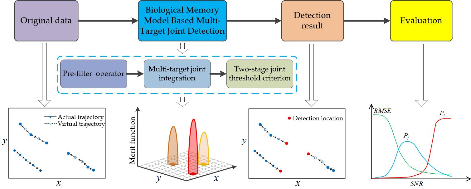
A biological memory model-based dynamic programming multi-target joint detection (BMM-DP-MJD) method is proposed. It detects multiple targets without pre-target and clutter information by means of an improved DP model, and adds biological memory model theory into the DP process to express the internal relationship of the flickering characteristics of the target among the frames and can deal with an unknown number of targets. The method includes four parts: a pre-detection operator, multi-target joint integration, and two-stage threshold judgment to achieve target detection. First, we use a global detection operator to discretize the multi-target state into multiple single-target states so as to realize the discretization of multiple targets. Second, the proposed function based on the biological memory model enhances the inter-frame correlation of targets with flickering characteristics. Then, the progressive loop integral operation in multi-target joint integration updates the merit function to optimize the target estimation set, reducing the interference and retaining useful information. Finally, the multi-target detection results are obtained by using the two-stage threshold criterion. Through the above steps, this paper makes the following two contributions:
  • Detection of the target with flickering characteristics under low SCR. This paper proposes a memory weight DP merit function integral operator. The theory of biological memory is introduced into DP integration to study the appearance and blanking state of targets with flickering characteristics in sea clutter. The merit function effectively integrates the correlation of flickering characteristic targets’ states among different frames. Therefore, the method achieves accurate detection for flickering characteristic targets with a low SCR.
  • Multi-target detection is employed without pre-target number information, and the computational cost is reduced. Usually, when using DP to solve multi-target detection problems, the target’s high-dimensional state is difficult to calculate due to the uncertain number of targets. However, the target number being known is inconsistent with practical applications. Therefore, we choose a simple and effective way to achieve the suboptimal solution of multi-target detection. We use a lower global threshold in the DP process and discretize the areas with candidate targets to simplify the high-dimensional maximization to multiple low-dimensional maximization, meaning that the computational cost is reduced.
This paper is organized as follows. Section 2 introduces the DP model. Section 3 describes the process of biological memory model-based dynamic programming multi-target joint detection method. Section 4 verifies the effectiveness of the algorithm through simulation data and experimental data analysis. Section 5 concludes the article.

2. DP Model

Because the DP model is the basic theory of the proposed method, Section 2 introduces the target motion model and the detection process of the DP target detection method [27].

2.1. Target Motion Model

The primary DP model is designed for a single target, and the multi-target motion model is more complicated. Therefore, this section assumes a point target for description. First, obtain the K frame’s monitoring area images I with the resolution cell N × N , then the motion model of the k - th frame target can be established as:
X ( k + 1 ) = Q X ( k ) ,   k < K ,
where
X ( k ) = [ x ( k ) x ¯ ( k ) y ( k ) y ¯ ( k ) ] , Q = [ 1 t 0 0 0 1 0 0 0 0 1 t 0 0 0 1 ] ,
where X ( k ) is the state vector, ( x ( k ) , y ( k ) ) represents the target location and ( x ¯ ( k ) , y ¯ ( k ) ) represents the target direction velocity at the k - th frame, Q is the state transition matrix, and t is the time interval between frames. Based on the above information, we can deduce the state transition equation that represents the possibility of the target location in different frame images.
At the k - th frame, define the merit function as M E ( k ) = { m e i j ( k ) } for 1 i , j N . It is utilized to describe the accumulation of target detection quantity, which is used to obtain the optimal estimate of the target in order to make the final detection decision. Placement function is defined as T ( k ) = { t i j ( k ) } for 1 i , j N . It describes the location of the candidate target, which corresponds to the merit function.

2.2. Multi-Frame Joint Target Detection

The multi-frame joint target detection result is obtained by joint processing the K frame images in this part. The algorithm is described as follows.

2.2.1. Initialization

Obtain the target state vector according to the maximum speed range of the ship. The initial merit function value is:
M E ( 1 ) = {   m e i j ( 1 ) = 0 } ,
The initial placement function value is:
T ( 1 ) = {   t i j ( 1 ) = 0 } ,

2.2.2. Multi-Frame Joint Integration

Start with the first state, with i = 1 ,   j = 1 at the second frame image, find the states and their respective probabilities at the first-frame image that leads to the current state according to the state transition equation. z m n ( 1 ) for 1 m ,   n N is the state that leads to the current state with maximum probability. Obtain the merit function:
M E 11 ( 2 ) = arg max M E ( 1 ) [ m e 11 ( 2 ) ] + z 11 ( 2 ) ,
The placement function value is:
T 11 ( 2 ) = C { m m n ( 1 ) } = ( m , n ) ,
where arg max M E ( 1 ) [ m e 11 ( 2 ) ] = m e m n ( 1 ) , and the placement function is C { m e i j ( x ) } = ( i , j ) .
For 3 k K , 1 i , j N , the merit function is updated:
M E i j ( k ) = arg max M E ( s 1 ) [ m e i j ( k ) ] + z i j ( k ) ,
Additionally, the placement function is updated:
T i j ( k ) = C { arg max M E ( s 1 ) [ m e i j ( k ) ] } ,
Repeat the above loop, and finally, the merit function accumulation result M E ( K ) and placement function result T ( K ) are obtained.

2.2.3. Target Detection

When there is a single target, the optimal estimate position is the position of maximum merit function shown in Formula (9).
B ( K ) = C { max M E ( K ) } ,
B ( K ) represents the optimal estimate position of the target in the K - th frame. Usually, when using DP to solve a single-target detection problem, it is simple to obtain the optimal estimate position of the target. However, if we use DP to solve multi-target detection problems, the target high-dimensional state is difficult to calculate due to the uncertain number of targets. Therefore, traditional DP has some limitations in solving multi-target detection.

3. Biological Memory Model Based Multi-Target Joint Detection Method

Due to the appearance and blanking state of flickering characteristic targets in sea clutter, the traditional DP method will suffer integration performance loss. The memory and forgetting process in the biological memory model can be an analogy for the appearance characteristics of the flickering characteristic targets. Therefore, this paper adds memory weights to imitate the scattering characteristics of the flickering characteristic targets in the DP algorithm, enlarging the inter-frame correlation of the flickering characteristic targets. Thus, the effective integration of the merit function can be obtained, realizing the accurate detection of the flickering characteristic targets. The following part will introduce the biological memory model and BMM-DP-MJD method in detail, and provide a discussion of particularly difficult situations.

3.1. Biological Memory Theory for the Flickering Characteristics Target

3.1.1. Definition of Memory and Forgetting

  • Memory
Memory is the reflection of the experience stored in the human brain. Figure 1 shows a schematic diagram for the memory of a single neuron. According to the process of stimulation and memory, the definition of an exponential function is more suitable for describing the memory process, and the formula of the memory function is written as [40]:
m m = ε × t δ ,
where m is the memory, t is the time interval, δ is the memory enhancement coefficient, and ε is the memory coefficient constant. Additionally, the memory increases faster when δ and ε becomes larger and vice versa.
Figure 1. The schematic diagram for the memory stimulus and responses. (a) Responses of two long-interval stimuli; (b) responses of two short-interval stimuli; (c) responses of three consecutive stimuli [40].
Remotesensing 14 00039 g001
  • Forgetting
The opposite of memory is forgetting, which means the memorized content cannot be retrieved. The formula of the forgetting function is [40]:
m f = × t β ,
where m is the memory, t is the time interval, β is the memory attenuation coefficient, and is the memory coefficient constant. Additionally, the memory forgets faster when β and becomes larger and vice versa.

3.1.2. The Memory Model for the Flickering Characteristics Target

The process of biological memory forgetting is similar to the scatter appearance characteristics of scintillating targets. When the flickering characteristic target is submerged in the clutter in the image, it is similar to the temporary forgetting process of memory. If the targets disappear for too long, it means that they no longer appear and cannot be recovered. The situation of temporary blanking and appearance is similar to the process of temporary forgetting and memory in the memory model. In the biological memory model, a repeat stimulus will improve the memory level, and a “repeat stimulus” is similar to the similarity of the target among frames. This paper considers the target similarity measure from two perspectives, namely target amplitude change and direction vector change. So, Formulas (9) and (10) are modified as:
m m = ε × t δ cos ( θ ) ,
m f = × t β ,
where m m and m f , respectively, represent the update coefficient function for the presence and blanking state of the flickering characteristic target. ε and represent the memory constant coefficient for the presence and blanking state, respectively. Additionally, the update coefficient function increases faster when δ and ε become larger, decreases faster when β and become larger and vice versa. t represents the frame concerned with the time interval, and cos ( θ ) represents the difference between two presence motion states of targets, which can be written as:
cos ( θ ) = a ¯ b ¯ | a ¯ | | b ¯ | ,
where a ¯ and b ¯ are the direction vectors of the two target states and | | represents the modular operation.

3.2. Process of BM-DP-MJD Method

The DP model presented in Section 2 is a single-target model. To achieve the accurate detection of flickering multi-targets, the pre-filter operator and the biological memory model are integrated into the DP model. The flowchart of the proposed method is shown in Figure 2—the colorful block diagram on the left shows the overall steps, the flowchart in the middle part of the diagram shows the specific process of the method, and the flowchart in the right part of the diagram shows the specific explanation for the multi-target joint iteration step.

3.2.1. Pre-Filter Operator

Assuming the number of images is K , and the resolution cell is N × N , for the K frame images I , the pre-filter step aims to eliminate non-target points in the images. The pre-filter operator is represented as [41]:
Z ( k ) = [ I ( k ) > mean ( I ( k ) ) ] ,                                   k K ,
where represents the scale factor, which is set as 0.7 in the paper, and mean ( ) is the averaging operator. After pre-filter operating, the K frame image set can be expressed as Z K = { Z ( 1 ) , ... , Z ( K ) } . Additionally, the discretized connected region of candidate targets in the k - th frame is denoted as Z ( k ) = { z i j 1 ( k ) , z i j 2 ( k ) , z i j l ( k ) , , z i j L ( k ) } , where i , j [ 1 , N ] , 1 l M . Then, the initial candidate M target number states are initially obtained according to the number of connected regions in Z k .
At the k - th frame, the l - th target is considered as a point moving with constant velocity in the x y plane, where the location is the coordinate of the maximum value in the l - th connected region. Formula (1) can thus be rewritten as:
X l ( k + 1 ) = Q X l ( k ) [ I i , j > T l ] ,               k < K ,
where
X l ( k ) = [ x l ( k ) x ¯ l ( k ) y l ( k ) y ¯ l ( k ) ] , Q = [ 1 t 0 0 0 1 0 0 0 0 1 t 0 0 0 1 ] ,
where X l ( k ) is the l - th target state vector, ( x l ( k ) , y l ( k ) ) represents the l - th target location, and ( x ¯ l ( k ) , y ¯ l ( k ) ) represents the l - th target direction velocity at the k - th frame. Then, the state transition equation can be deduced, which represents the possibility of the ship’s location being in different frame images.

3.2.2. Multi-Target Joint Integration

In this part, we obtained multi-target detection results through K frames image joint processing. The algorithm is as follows:
1.
Initialization
Obtain the target state vector according to the maximum speed range of the ship, for the target in 1 - th frame, and Formulas (3) and (4) can be written as:
M E l ( 1 ) = {   m e i j l ( 1 ) = 0 } ,
T l ( 1 ) = {   t i j l ( 1 ) = 0 } ,
For the 1 - th frame, the l - th target dynamic motion matrix can be modeled by:
X l ( 1 ) = [ x l ( 1 ) ,   x ¯ l ( 1 ) ,   y l ( 1 ) ,   y ¯ l ( 1 ) ] ,
2.
Multi-frame joint accumulation
Starting with the first state of the second image, the state of the current frame and their respective probabilities are found in the first frame image according to the state transfer equation. z m , n l ( 1 ) is the state that leads to the current state with maximum probability. To combine the biological memory update coefficient function, a flag is needed to indicate whether there is a candidate target in the next frame relevant area. So, the flag ξ is set as:
{ ξ = 1 ;   a   candidate   target ξ = 0 ;   no   candidate   target   ,
where ξ = 1 means the next frame has a candidate target, while ξ = 0 means the next frame does not have a candidate target.
Combined with the update function based on the biological memory model proposed in Section 3.1, the second frame merit function (Formula (5)) is rewritten as follows for the l - th target:
M E l ( 2 ) = { arg max M E l ( 1 ) [ m e l ( 2 ) ] +   z i j l ( 2 ) ε × κ m δ cos 2 l ( θ ) ;   ξ = 1   arg max M E l ( 1 ) [ m e l ( 2 ) ] + z i j l ( 2 ) × κ f β ;   ξ = 0 ,
where arg max M E m ( 1 ) [ m e l ( 2 ) ] = m e m n l ( 1 ) , δ and β represent the number of continuous presence or blanking states, κ m indicates the number of times that the candidate target demonstrates a continuous presence, and κ f indicates the number of times that the candidate target occupies a blanking state. At the same time, the placement function is expressed as:
T l ( 2 ) = C { m e m n l ( 1 ) } = ( m , n ) ,
and
cos 2 l ( θ ) = ( x ¯ l ( 2 ) ) 2 + ( y ¯ l ( 2 ) ) 2 x ¯ l ( 2 ) y ¯ l ( 2 ) ,
For the second frame, the state transition matrix updates with the first frame matrix:
X l ( 2 ) = { [ x l ( 2 ) = x l ( 2 )   x ¯ l ( 2 ) = x l ( 2 ) x l ( 1 )     y l ( 2 ) = y l ( 2 )     y ¯ l ( 2 ) = y l ( 2 ) y l ( 1 ) ] ;                 ξ = 1   [ x l ( 2 ) = x l ( 2 )   x ¯ l ( 2 ) = 2 x ¯ l ( 2 )     y l ( 2 ) = y l ( 2 )     y ¯ l ( 2 ) = 2 y ¯ l ( 2 ) ] ;                 ξ = 0     ,
If there is a candidate target in the second frame, the velocity vector is the difference between the target position of the first frame and the target position of the second frame. Otherwise, the new velocity vector is twice the initial velocity vector.
Repeat the above steps for all states at the second-frame image to obtain M E ( 2 ) and T ( 2 ) . Then, x ( 2 ) is renewed as the second frame state. For 3 k K , l L , the state transition matrix will be updated with the information of the first two frames:
X l ( k ) = { [ x l ( k ) = x l ( k )   x ¯ l ( k ) = x ¯ l ( k 1 ) x ¯ l ( k 2 )     y l ( k ) = y l ( k )     y ¯ l ( k ) = y ¯ l ( k 1 ) y ¯ l ( k 2 ) ] ;     ξ = 1 [ x l ( k ) = x l ( k 1 )   x ¯ l ( k ) = x ¯ l ( k 1 )   y l ( k ) = y l ( k 1 )     y ¯ L ( k ) = y ¯ L ( k 1 ) ] ;   ξ = 0   ,
If there is a candidate target in the k - th frame, the velocity vector is represented as the difference between ( k 1 ) - th frame target position and ( k 2 ) - th frame target position. Otherwise, the new velocity vector is the same as the previous velocity vector.
The Merit function is:
M E l ( k ) = { arg max M E l ( k 1 ) [ m e l ( k ) ] + z i j l ( k ) ε × κ δ cos k l ( θ )   ;   ξ = 1   arg max M E l ( k 1 ) [ m e l ( k ) ] + z i j l ( k ) × κ β ;   ξ = 0 ,
Additionally, the placement function is:
T l ( k ) = C { arg max M E ( k 1 ) [ m e l ( k ) ] } ,
3.
Progressive loop integration
The result of the pre-filtering operator of the k - th frame is utilized to update the candidate target number L . Additionally, step B is repeated, and finally, the merit function result M E ( K ) and placement function result T ( K ) are obtained.

3.2.3. Two-Stage Joint Threshold Criterion

As we all know, there are many types of targets in the water. We can divide them into two categories to achieve threshold segmentation—the highest merit function value and the second-highest merit function value represent continuous strong targets and flickering characteristic targets, respectively. Therefore, a two-stage threshold criterion is utilized to obtain the final detection result.
First, the global detection threshold determines whether the target exists:
B S ( K ) = C { M E ( K ) > γ S } ,
where γ S = K m e a n ( ( K Z ( k ) ) / K ) K 4 , and m e a n ( ( K I ( k ) ) / K ) indicates the average energy of the image. Because continuous strong targets and flickering characteristic targets differ greatly, a high threshold is first used to detect candidate continuous strong targets:
B h ( K ) = C { M E ( K ) > γ h } ,
where B h ( K ) indicates the most likely position of a continuous strong target (such as a cargo ship, liner) in the K - th frame image. Additionally, γ h = K m e a n ( ( K Z ( k ) ) / K ) K 2 represents the high threshold. Then, the continuous strong targets are removed from the set of candidate targets. For the rest of the candidate targets, the M candidate region is ranked to carry out the subtraction. The continuous difference on all samples is carried out, and the midpoint of the largest difference as the threshold γ is chosen to realize the detection of flickering characteristic targets, as shown in Figure 3:
B f ( K ) = C { M m ( K ) > γ } ,
Finally, the detection result is detected by the two-stage threshold criterion, and the placement set B ( K ) = B h ( K ) + B f ( K ) is obtained.
Figure 3. The schematic diagram of sorting detection step.
Remotesensing 14 00039 g003

3.3. Assumptions for Special Situations of Flickering Characteristics Multi-Target Detection

In order to compare the difference between the integral of the multi-target and the single-target, some specific analysis is carried out. In actuality, the assumption that all targets are far from each other is too strict. It is important to have the ability to deal with difficult situations for detection systems in practical applications such as target trajectory crossing. The following sections introduce three types of flicking characteristic multi-target assumptions, and we will analyze them one by one.
Assumption 1: When two targets have trajectories that cross, one of the target states disappears, as shown in Figure 4a. S 1 is the motion area of target 1, and is the same as S 2 . Target 2 may be incorrectly associated with the trajectory of target 1 due to the disappearing state. However, its direction vector has undergone some change. Therefore, the correlation threshold is set to avoid spurious correlation.
Assumption 2: For the situation where two targets have trajectories that cross, both target states disappear, as shown in Figure 4b. As mentioned above, the correlation threshold is set to avoid spurious correlation.
Assumption 3: Targets in proximity and that are indistinguishable are rare in reality, but they can be regarded as one target in the navigation radar if it happens. When two targets have approximately parallel trajectories, both target states disappear, as shown in Figure 4c. Target 1 may be incorrectly associated with the trajectory of target 2 due to the empty state. However, its direction vector has undergone some change. The accumulation becomes smaller, and its merit function will be lower than the final detection threshold.

4. Results and Discussion

4.1. Simulation Data Results

In this subsection, simulation results are provided to verify the effectiveness of the proposed method, including simulation data results in demonstration detection results and performance analysis. The clutter distribution in the simulation was modeled as K distribution [31]:
p ( ζ k ) = 2 β Γ ( α ) ( β ζ k 2 ) K α 1 ( β ζ k ) ,
where α is the shape parameter of the distribution, β is the scale parameter, and K α 1 ( ) was the modified second-kind Bessel function of order α 1 . Three kinds of targets were considered, including uniform distribution targets, binomial distribution targets, and Swerling I distribution targets. Uniform distribution targets represent targets with a continuous state and stable energy. Swerling I distribution targets and binomial distribution targets were utilized to provide an analogy for two types of flickering characteristic targets. Swerling I distribution targets represent the target with energy fluctuations, and binomial distribution targets represent the targets with an appearance and blanking state. Their probability distribution functions are given in the following [42].
For the uniform distribution target, the probability distribution functions can be expressed as:
P ( I k ) = I k a b a , a I k b ,
where a and b are the frame range of data. This indicates that the target appearance probability is the same, and the amplitude of the target is fixed.
For the binomial distribution target, the probability distribution functions can be expressed as:
P ( I k = 1 ) = C ( n k , l ) p l ( 1 p ) n k l ,
C ( n k , l ) = n k ! l ! ( n k l ) ! ,
where C ( n k , l ) is the binomial coefficient, n k is the total length of the sequence, l is the target amplitude I k = 1 , and p is the probability when the number of I k = 1 is l .
For the Swerling I distribution target, the probability distribution functions can be expressed as:
P ( I k ) = 2 I k σ ¯ exp ( ( I k ) 2 σ ¯ ) ,
where σ ¯ represents the target mean square amplitude. For the designed target trajectory, the trajectory random noise is added, and the variance σ 2 and mean E are shown in Table 1. Additionally, the other parameters in the simulation are shown in Table 1, too.
To evaluate the detection performance of the proposed method, the specific indicators are shown as follows:
Target detection probability P d : the probability that the last stage positions of the estimated state are within two cells of the actual target location.
P d = 1 M m = 1 M [ S m = B ^ m ( K ) 2 B m ( K ) 2 < 2 ] ,
where B ^ m ( K ) is the estimated target position of m - th , and B m ( K ) is the actual target position of m - th .
The false alarm probability P f a : the probability of reporting at least one false position when no target appears,
P f a = 1 M m = 1 M [ S m = B ^ m ( K ) 2 B m ( K ) 2 > 2 ] ,
The root mean square error (RMSE) of position: the average position difference between the estimated state of the valid target detection and the discretized state of the real target.
RMSE = 1 M m = 1 M [ B ¯ ^ m ( K ) 2 B ¯ m ( K ) 2 ] ,
where B ¯ ^ m ( K ) represents the target position coordinate correctly estimated by m - th , and B ¯ m ( K ) represents its actual target position coordinate.

4.1.1. Demonstration of Simulation Data Detection Results

First, simulation data demonstrated the detection process of the proposed method. Figure 5 shows the data generation and process of BMM-DP-MJD intuitively. Figure 5a shows the target generation model—there are five targets, and the target parameters are shown in Table 2. Figure 5b–e shows the simulation data, and the target states in the different frames are marked with different color circles. As expected, targets with SCR = 10 dB are much more obvious than targets with SCR = 5 dB, and in addition, targets with SCR = 5 dB disappear from sight in some frames due to their flickering characteristics. For example, Target 1 disappears in the third and fourth frames. Additionally, Figure 6a shows the decision process of the detection threshold criterion. Because of the above-mentioned complex situations, strict target threshold criteria are required to remove false alarms as much as possible. Lastly, the 2D and 3D diagrams of the merit function value in 10 frames are shown in Figure 6b,c, respectively. These diagrams show that five targets were accumulated in the merit function, and in addition, two flickering characteristic targets’ merit functions were lower than the high targets. The results show that BMM-DP-MJD has the ability to enhance the flickering characteristic targets’ merit function integral among the frames, thereby improving the ability to extract the flickering characteristic targets from the image with high-scattering targets.

4.1.2. Simulation Data Detection Performance of BMM-DP-MJD

Then, three types of targets distribution are modeled to verify the detection performance. Additionally, 200 Monte Carlo runs are performed for each test.
  • Detection performance of three types of target
Six separate targets are considered to verify the multiple target detection performance of BMM-DP-MJD for three types of target. The false alarm probability and the RMSE of the six targets after applying BMM-DP-MJD methods are also considered. The distribution types of the six targets are shown in Table 3. Figure 7a presents the target generation model, and Figure 7b–d shows the detection probability. Its characteristics are consistent with the above description. Overall, the detection probability of all targets approaches 1 as the target SCR increases, and the detection probability’s max difference is 0.25 with the same SCR among the six targets. In particular, when SCR = 8 dB, the detection probability can generally reach 0.8; the RMSE is less than 0.2 cells; the false alarm probability of a uniform distribution target and a binomial distribution target is less than 0.3, and the false alarm probability of a Swerling I distribution target is about 0.4. It should be noted that different from binomial distribution and uniform distribution targets, the detection performance of Swerling I distribution targets is lower with the proposed method when SCR is 5–10 dB. Moreover, the false alarm probability of Swerling I distribution targets is slightly higher than the other types. The reason for this is that the energy fluctuation range of the target with Swerling I distribution is unstable.
  • Detection performance in special assumed situations
In Section 3.3, the special situations with several types of assumptions are explained. Here, the detection performance of the proposed method is simulated with these assumptions. Figure 8a is the target generation model, and the parameters of the specific situation are shown in Table 4. Target 1 and target 2 correspond to assumptions 1 and 2 in Section 3.3; target 3 and target 4 correspond to assumptions 3; target 5 is a comparison item. Figure 8b–d, respectively, show the detection probability, RMSE, and false alarm probability of these five targets with the BMM-DP-MJD method. When SCR = 8 dB, the detection probability can reach 0.9; the RMSE is relatively stable, at less than 0.25 cells; the false alarm probability is less than 0.42. It should be noted that the two special situations have some loss in detection performance compared with comparison target 5. Therefore, the proposed method has effective detection performance for the special situations described in Section 3.3.
  • Comparison of the detection performance of three algorithms on simulation data
For this part, the performances of the DP-TBD [27], two-Stage DP-TBD [28], and the proposed BMM-DP-MJD are investigated. The proposed BMM-DP-MJD method is analyzed qualitatively and quantitatively to verify the effectiveness of the method for the detection of flickering characteristic multi-targets under a low SCR.
Firstly, the detection probability, the false alarm probability, and the RMSE of the target position of these three methods mentioned above with three types of target are shown in Figure 9. Figure 9a–c shows the detection probability performance curves of the three different types of target. Figure 9d–f shows the RMSE performance curves of the three different types of target. Figure 9g–i presents the false alarm probability performance curves of three different types of target. It can be observed that the detection results of all targets approach 1 as the target SCR increases. Overall, this shows the excellent detection performance of the proposed method. When SCR = 8 dB, the detection probability can generally reach 0.9; the false alarm probability is below 0.3; the RMSE of the uniform distribution target and the binomial distribution is less than 0.3 cells, and the RMSE of the Swerling I distribution target is about 0.4 cells. It is worth noting that the detection performance is better for Swerling I distribution with the proposed method when SCR ranges from 3 to 5 dB. The reason for this is that the amplitude of Swerling I distribution targets obeys an exponential distribution, and the merit function suddenly increases for some high and continuous target states in batches with the memory weight.
Another experiment is simulated to verify the detection performance of this method for flickering characteristics targets with another test. Figure 10 shows the target detection performance curves of the three methods with different binomial probability distributions under SCR = 8 dB. By changing the distribution parameters, the change in the flickering characteristic target is modeled. Figure 10a–c depicts the performance curves of the detection probability, RMSE, and false alarm probability of the three methods for a single target with the change in the binomial distribution parameters. In general, the method in this paper has a better detection performance curve. For this method, when the binomial distribution probability is 0.6, the detection probability can reach 0.85, the RMSE is less than 0.3 cells, and the false alarm probability is less than 0.42.
Above all, the simulation data show three different DP methods to solve the flickering characteristic multi-target detection problem under an SCR of 3–8 dB. So, the BMM-DP-MJD method was analyzed qualitatively and quantitatively from aspects such as generalization, accuracy, and SCR, which verified the effectiveness of the method for detecting flickering characteristic targets.

4.2. Experimental Data Detection Performance of BMM-DP-MJD

In this subsection, experimental results are provided to validate the effectiveness of the proposed method. The parameters of the experimental data are shown in Table 5. Figure 11a presents a satellite map of the experimental area. The imaging scenario is shown in Figure 11d. There is a river, and there are multiple buildings located on both sides of the river. In the river, there are five targets of interest in the scenario. A batch dataset of nine frames with processed echo is shown in Figure 11b,c,e,f. Target 1 and target 2 are ships, which are marked with red and yellow circles separately. Target 3, target 4, and target 5 are three marker buoys located in the mid-tail of the river, which are marked with green, black, and grey circles separately. Obviously, the size of ships is much bigger than that of the marker buoys. In addition, marker buoys are weaker than the ships and they do not appear continuously in the images, as shown in Figure 11b,c,e,f. We can see that the weak targets of target 3, target 4, and target 5 disappear in the seventh frame and target 5 disappears in the last frame.
Figure 12a–f presents the merit function in 3D graphs and the detection results of the three methods. It can be seen that the two ships were easy to integrate, but the three methods have different results for the buoy shown in Figure 12a–c. Finally, after two-level threshold discrimination, the three detection results of the above method were obtained, as shown in Figure 12d–f. DP-TBD only detected two ships, while two-level DP-TBD detected two ships and two buoys, but lost one buoy and had two false alarms. In the BMM-DP-MJD detection result, there are five targets, which correspond to the actual targets. The average specific detection indicators of the five targets are shown in Table 6. In the experimental data, five targets are detected correctly by the proposed method, which is more than 0.2 higher than the other two methods; the false alarm probability of the BMM-DP-MJD is 0, which is 0.4 lower than Two-Stage DP-TBD; the RMSE of the BMM-DP-MJD is 1.7 cells, which is more than nine cells lower than the other two methods. This verifies the ability of the proposed BMM-DP-MJD method in the accurate detection of flickering characteristic multi-targets.

4.3. Detection Performance Discussion

From the simulation data result, for three different distribution targets, the detection probability of BMM-DP-MJD can reach 0.91 when SCR = 8 dB. This is 0.1 higher than the two-stage DP method. And the RMSE of the proposed method is about 0.4 cells, which is 0.1 lower than the two-stage DP method. In the experimental data, five targets are correctly detected by the proposed method, whose detection probability is more than 0.2 higher than that of the other two methods; the false alarm probability of the BMM-DP-MJD is 0, which is 0.4 lower than Two-Stage DP-TBD; the RMSE of the BMM-DP-MJD is 1.7 cells, which is more than nine cells lower than the other two methods.
Because the proposed method adds the exponential order integral of the state of existence target, the weak targets can be accumulated to a greater extent than other methods. So, there is a difference among the detection results. Therefore, the detection results of simulation data and experimental data illustrated that the proposed method exhibits a better detection performance for targets with flickering characteristics under a low SCR, thereby improving the target detection effectiveness of marine navigation radar.

5. Conclusions

This paper proposes a multi-frame joint detection algorithm, named BMM-DP-MJD, for a new type of fluctuating target on river and sea surfaces, which demonstrates flickering characteristics. The pre-filtering operator realizes the multi-target DP with an unknown target state. Moreover, the method utilizes the integration capability of BMM-DP-MJD based on memory weights to yield accurate detection results for fluctuating targets with flickering characteristics. Simulation data illustrated that the detection performance of the proposed method greatly improved for targets with flickering characteristics under a low SCR of 3–8 dB. Moreover, the experimental data reveal that ship and small buoy targets were accurately detected by the proposed method in the river, thereby improving the target detection effectiveness of marine navigation radar.
In this study, we discuss the detection of flickering characteristic targets with the hypothesis of point targets, and so target features such as shapes and local amplitude distribution did not participate in the detection process. In the future, the influence of target features such as shape and local amplitude distribution on detection performance will be further investigated. Moreover, the effects of sources of noise such as storms and heavy rain will be considered in further research.

Author Contributions

Conceptualization, Q.Z. and W.H.; methodology, Q.Z. and W.H.; writing—original draft preparation, Q.Z.; writing—review and editing, J.P.; funding acquisition, Y.H. and J.P.; project administration, J.Y.; Data curation, Y.Z. and J.P. All authors have read and agreed to the published version of the manuscript.

Funding

This research was funded by the National Natural Science Foundation of China, grant number 61901091 (Jifang Pei), 61901090(Yin Zhang), 61671117(Yulin Huang).

Conflicts of Interest

The authors declare no conflict of interest.

References

  1. Huo, W.; Tuo, X.; Zhang, Y. Balanced Tikhonov and Total Variation Deconvolution Approach for Radar Forward-Looking Super-Resolution Imaging. IEEE Geosci. Remote Sens. Lett. 2021, 19, 3505805. [Google Scholar] [CrossRef]
  2. Zhang, Y.; Luo, J.; Li, J. Fast Inverse-Scattering Reconstruction for Airborne High-Squint Radar Imagery Based on Doppler Centroid Compensation. IEEE Trans. Geosci. Remote Sens. 2021, 60, 5205517. [Google Scholar] [CrossRef]
  3. Hao, C.P.; Li, J.; Hou, C.H. A Study on CFAR Detection Method of Weighted Cell Averaging and Fuzzy Rules. Modern Radar 2009, 31, 44–46. [Google Scholar]
  4. De Maio, A.; Foglia, G.; Conte, E. CFAR behavior of adaptive detectors: An experimental analysis. IEEE Trans. Aerosp. Electron. Syst. 2005, 41, 233–251. [Google Scholar] [CrossRef]
  5. Leng, X.; Ji, K.; Yang, K.; Zou, H. A bilateral CFAR algorithm for ship detection in SAR images. IEEE Geosci. Remote Sens. Lett. 2015, 12, 1536–1540. [Google Scholar] [CrossRef]
  6. Miao, K.; Leng, X.; Zhao, L.; Ji, K. A modified faster R-CNN based on CFAR algorithm for SAR ship detection. In Proceedings of the 2017 International Workshop on Remote Sensing with Intelligent Processing (RSIP), Shanghai, China, 18–21 May 2017; pp. 1–4. [Google Scholar]
  7. Fang, X.U.; Jing-Hong, L. Ship detection and extraction using visual saliency and histogram of oriented gradient. IEEE Geosci. Remote Sens. Lett. 2016, 12, 473–477. [Google Scholar]
  8. Chen, Y.; Xin, Y. An efficient infrared small target detection method based on visual contrast mechanism. IEEE Geosci. Remote Sens. Lett. 2016, 13, 962–966. [Google Scholar] [CrossRef]
  9. Han, J.; Yong, M.; Bo, Z.; Fan, F.; Liang, K.; Yu, F. A robust infrared small target detection algorithm based on human visual system. IEEE Geosci. Remote Sens. Lett. 2014, 11, 2168–2172. [Google Scholar]
  10. Chen, S.; Wang, H.; Xu, F. Target classification using the deep convolutional networks for SAR images. IEEE Trans. Geosci. Remote Sens. 2016, 54, 4806–4817. [Google Scholar] [CrossRef]
  11. Liu, J.; Feng, Y.; Liu, W.; Orlando, D.; Li, H. Training data assisted anomaly detection of multi-pixel targets in hyperspectral imagery. IEEE Trans. Signal Proc. 2020, 68, 3022–3032. [Google Scholar] [CrossRef]
  12. Lang, H.; Jie, Z.; Xi, Z.; Meng, J. Ship classification in SAR image by joint feature and classifier selection. IEEE Geosci. Remote Sens. Lett. 2015, 13, 212–216. [Google Scholar] [CrossRef]
  13. Chen, C.P.; Li, H.; Wei, Y.; Xia, T.; Tang, Y.Y. A local contrast method for small infrared target detection. IEEE Trans. Geosci. Remote Sens. 2013, 52, 574–581. [Google Scholar] [CrossRef]
  14. Wang, X.; Chen, C. Adaptive ship detection in SAR images using variance WIE-based method. Signal Image Video Processing 2016, 10, 1219–1224. [Google Scholar] [CrossRef]
  15. Tao, W.; Guang-Shun, H.; Jing, G. Energy consumption and economic growth in China’s marine economic zones-an estimation based on partial linear model. Energy 2020, 205, 118028. [Google Scholar] [CrossRef]
  16. Gini, F.; Greco, M.V.; Diani, M.; Verrazzani, L. Performance analysis of two adaptive radar detectors against non-Gaussian real sea clutter data. IEEE Trans. Aerosp. Electron. Syst. 2000, 36, 1429–1439. [Google Scholar]
  17. Xu, S.; Zhu, J.; Jiang, J. Sea-surface floating small target detection by multifeature detector based on isolation forest. IEEE J. Sel. Top. Appl. Eart. Observ. Remote Sens. 2020, 14, 704–715. [Google Scholar] [CrossRef]
  18. Xu, X.K. Low observable targets detection by joint fractal properties of sea clutter: An experimental study of IPIX OHGR datasets. IEEE Trans. Ant. Prop. 2010, 58, 1425–1429. [Google Scholar]
  19. Shi, S.N.; Shui, P.L.; Liu, M. Subband adaptive coherent detection of weak moving targets in K-distributed sea clutter. In Proceedings of the 2016 CIE International Conference on Radar (RADAR), Guangzhou, China, 10–13 October 2016; pp. 1–4. [Google Scholar]
  20. Shui, P.L.; Li, D.C.; Xu, S.W. Tri-feature-based detection of floating small targets in sea clutter. IEEE Trans. Aerosp. Electron. Syst. 2014, 50, 1416–1430. [Google Scholar] [CrossRef]
  21. Xu, S.; Zheng, J.; Jia, P.; Shui, P. Sea-surface floating small target detection based on polarization features. IEEE Geosci. Remote Sens. Lett. 2018, 15, 1505–1509. [Google Scholar] [CrossRef]
  22. Shi, S.; Shui, P. Sea-surface floating small target detection by one-class classifier in time-frequency feature space. IEEE Trans. Geosci. Remote Sens. 2018, 56, 6395–6411. [Google Scholar] [CrossRef]
  23. Li, Y.; Xie, P.; Tang, Z.; Jiang, T.; Qi, P. SVM-based sea-surface small target detection: A false-alarm-rate-controllable approach. IEEE Geosci. Remote Sens. Lett. 2019, 16, 1225–1229. [Google Scholar] [CrossRef] [Green Version]
  24. Guo, Z.X.; Shui, P.L. Anomaly Based Sea-Surface Small Target Detection Using K-Nearest Neighbor Classification. IEEE Trans. Aerosp. Electron. Syst. 2020, 56, 4947–4964. [Google Scholar] [CrossRef]
  25. Li, D.; Shui, P. Floating small target detection in sea clutter via normalised Hurst exponent. Electron. Lett. 2014, 50, 1240–1242. [Google Scholar] [CrossRef]
  26. Barniv, Y.; Kella, O. Dynamic programming solution for detecting dim moving targets part II: Analysis. IEEE Trans. Aerosp. Electron. Syst. 1987, AES-23, 776–788. [Google Scholar] [CrossRef]
  27. Li, Y.; Li, W.; Yi, W. A distributed asynchronous recursive filtering fusion algorithm via DP-TBD. J. Radars 2018, 7, 254–262. [Google Scholar]
  28. Gao, J.; Du, J.; Wang, W. Radar detection of fluctuating targets under heavy-tailed clutter using track before detect. Sensors 2018, 18, 2241. [Google Scholar] [CrossRef] [Green Version]
  29. Yi, W.; Morelande, M.R.; Kong, L.J.; Yang, J.Y. An efficient particle filter for multi-target tracking using an independence assumption. In Proceedings of the 2012 15th International Conference on Information Fusion, Singapore, 9–12 July 2012; pp. 2378–2385. [Google Scholar]
  30. Jiang, H.; Yi, W.; Cui, G.; Kong, L.; Yang, X. Tracking targets in K clutter via particle filter. In Proceedings of the 2015 IEEE Radar Conference (RadarCon), Arlington, VA, USA, 10–15 May 2015; pp. 0350–0355. [Google Scholar]
  31. Huo, W.; Pei, J.; Huang, Y. A new maritime moving target detection and tracking method for airborne forward-looking scanning radar. Sensors 2019, 19, 1586. [Google Scholar] [CrossRef] [Green Version]
  32. Si, W.; Zhu, H.; Qu, Z. Robust Poisson multi-Bernoulli filter with unknown clutter rate. IEEE Access 2019, 7, 117871–117882. [Google Scholar] [CrossRef]
  33. Wang, W.; Sun, Z.; Li, C.; Wang, J. Study on dim target detection and discrimination from sea clutter. China Ocean Eng. 2013, 27, 183–192. [Google Scholar] [CrossRef]
  34. Grossi, E.; Lops, M.; Venturino, L. A novel dynamic programming algorithm for track-before-detect in radar systems. IEEE Trans. Signal Proc. 2013, 61, 2608–2619. [Google Scholar] [CrossRef]
  35. Orlando, D.; Ricci, G.; Bar-Shalom, Y. Track-before-detect algorithms for targets with kinematic constraints. IEEE Trans. Aerosp. Electron. Syst. 2011, 47, 1837–1849. [Google Scholar]
  36. Huang, D.; Xue, A.; Guo, Y. Penalty dynamic programming algorithm for dim targets detection in sensor systems. Sensors 2012, 12, 5028–5046. [Google Scholar] [CrossRef]
  37. Buzzi, S.; Lops, M.; Venturino, L.; Ferri, M. Track-before-detect procedures in a multi-target environment. IEEE Trans. Aerosp. Electron. Syst. 2008, 44, 1135–1150. [Google Scholar]
  38. Orlando, D.; Venturino, L.; Lops, M. Track-before-detect strategies for STAP radars. IEEE Trans. Signal Proc. 2009, 58, 933–938. [Google Scholar]
  39. Jiang, H.; Yi, W.; Cui, G. Knowledge-Based Track-Before-Detect Strategies for Fluctuating Targets in K-Distributed Clutter. IEEE Sens. 2016, 16, 7124–7132. [Google Scholar] [CrossRef]
  40. Morimoto, B.H.; Koshland, D.E. Short-term and long-term memory in single cells. FASEB 1991, 5, 2061–2067. [Google Scholar] [CrossRef] [PubMed]
  41. Gao, G.; Liu, L.; Zhao, L. An adaptive and fast CFAR algorithm based on automatic censoring for target detection in high-resolution SAR images. Trans. Geosci. Remote Sens. 2008, 47, 1685–1697. [Google Scholar]
  42. Cam, L.; Neyman, J.; Scott, E.L. Probability Theory; University of California Press: Berkeley, CA, USA, 1972. [Google Scholar]
Figure 2. The flowchart of the BMM-DP-MJD method.
Remotesensing 14 00039 g002
Figure 4. Assumptions for special situations of flickering characteristic multi-target detection. (a) Assumption 1; (b) assumption 2; (c) assumption3.
Remotesensing 14 00039 g004
Figure 5. Simulation data scenario of five targets. (a) The target generation model; (b) the first frame imaging; (c) the third frame imaging; (d) the fourth frame imaging; (e) the tenth frame imaging.
Remotesensing 14 00039 g005aRemotesensing 14 00039 g005b
Figure 6. Simulation data detection results of BMM-DP-MJD. (a) Decision program of detection threshold; (b) detection results of BMM-DP-MJD in 2-D; (c) detection results of BMM-DP-MJD in 3-D.
Remotesensing 14 00039 g006
Figure 7. The detailed detection performance of 6 separate targets. (a) Simulation scene of the of 6 separated targets; (b) the Pd of 6 separate targets; (c) the RMSE of 6 separate targets; (d) the P f a of 6 separate targets.
Remotesensing 14 00039 g007
Figure 8. The detection performance in assumed special situations. (a) Simulation scene of assumed situations; (b) the Pd of assumed situations; (c) the RMSE of assumed situations; (d) the P f a of assumed situations.
Remotesensing 14 00039 g008
Figure 9. Performance curves of the three methods. (a) The Pd of the uniform distribution target; (b) the P d of the binomial distribution target; (c) the P d of the Swerling I distribution target; (d) the RMSE of the uniform distribution target; (e) the RMSE of the binomial distribution target; (f) the RMSE of the Swerling I distribution target; (g) the P f a of the uniform distribution target; (h) the P f a of the binomial distribution target; (i) the P f a of the Swerling I distribution target.
Remotesensing 14 00039 g009
Figure 10. The detection performance curve of the three methods for the target with different binomial probability distributions under SCR = 8 dB. (a) The P d of targets under different binomial probability distributions; (b) the RMSE of targets under different binomial probability distributions; (c) the P f a of targets under different binomial probability distributions.
Remotesensing 14 00039 g010
Figure 11. Experimental data of navigation radar. (a) Experimental scene of the measured data; (b) the 1st-frame imaging; (c) the 3rd-frame imaging; (d) optical scene of the measured data; (e) the 7th-frame imaging; (f) the 9th-frame imaging.
Remotesensing 14 00039 g011
Figure 12. The experimental results of the methods mentioned. (a) Merit function results of DP-TBD; (b) merit function results of two-Stage DP-TBD; (c) merit function results of BMM-DP-MJD; (d) results of DP-TBD; (e) results of two-Stage DP-TBD; (f) results of BMM-DP-MJD.
Remotesensing 14 00039 g012
Table 1. The simulation data parameters.
ParameterValue
K distribution scale parameter α = 2 ,   β = 1
Number of frames 10
False alarm probability0.02
Target appearance’s probability of binomial distribution0.7
The size of simulation data 60 × 60
Target position random noise σ 2 = 1 ,   E = 0.001 c e l l
Table 2. Simulation target parameters.
Target NumberSCRDistribution
Target 15 dBSwerling I distribution
Target 210 dBUniform distribution
Target 310 dBUniform distribution
Target 45 dBSwerling I distribution
Target 510 dBUniform distribution
Table 3. The distribution of three types of target.
Target NumberDistribution
Target 1, Target 4Binomial distribution
Target 2, Target 5Swerling I distribution
Target 3, Target 6Uniform distribution targets
Table 4. The distribution of targets in special assumed situations.
Target NumberDistribution
Target 1The target disappearance probability is 0.2
Target 2Binomial distribution
Target 3The target disappearance probability is 0.3
Target 4Binomial distribution
Target 5Binomial distribution
Table 5. The parameters of the experimental data.
ParameterValueParameterValue
Wave band X bandMain lobe of the azimuth 5.1°
Scanning speed72°/sBandwidth75 MHz
PRF200 HzImage size 1500 × 256
Table 6. The detection result of experimental data.
Method P d P f a RMSE (Cell)
DP-TBD 0.4011.3 of 1500 × 256
Two stage DP-TBD0.80.414.3 of 1500 × 256
BMM-DP-MJD101.7 of 1500 × 256
Publisher’s Note: MDPI stays neutral with regard to jurisdictional claims in published maps and institutional affiliations.

