Fast Urban Land Cover Mapping Exploiting Sentinel-1 and Sentinel-2 Data

Abstract

The rapid change and expansion of human settlements raise the need for precise remote-sensing monitoring tools. While some Land Cover (LC) maps are publicly available, the knowledge of the up-to-date urban extent for a specific instance in time is often missing. The lack of a relevant urban mask, especially in developing countries, increases the burden on Earth Observation (EO) data users or requires them to rely on time-consuming manual classification. This paper explores fast and effective exploitation of Sentinel-1 (S1) and Sentinel-2 (S2) data for the generation of urban LC, which can be frequently updated. The method is based on an Object-Based Image Analysis (OBIA), where one Multi-Spectral (MS) image is used to define clusters of similar pixels through super-pixel segmentation. A short stack (<2 months) of Synthetic Aperture Radar (SAR) data is then employed to classify the clusters, exploiting the unique characteristics of the radio backscatter from human-made targets. The repeated illumination and acquisition geometry allows defining robust features based on amplitude, coherence, and polarimetry. Data from ascending and descending orbits are combined to overcome distortions and decrease sensitivity to the orientation of structures. Finally, an unsupervised Machine Learning (ML) model is used to separate the signature of urban targets in a mixed environment. The method was validated in two sites in Portugal, with diverse types of LC and complex topography. Comparative analysis was performed with two state-of-the-art high-resolution solutions, which require long sensing periods, indicating significant agreement between the methods (averaged accuracy of around 90%).

1. Introduction

In recent decades, mapping urban areas and growth has been a vital tool in facing many environmental challenges. The task is usually well performed by high-resolution MS remote sensing instruments [1]. However, such data resources are often costly and unavailable to common users. The recent increase in the availability of open-access satellite data has given rise to the need for algorithms that can exploit moderate-resolution images.

The ability to track the evolution of urban fabrics in real-time is another crucial consideration due to the fast urbanization processes experienced worldwide. MS-based solutions usually require multi-temporal stacks due to the wide heterogeneity of anthropic structures and variations in illumination conditions [2,3,4]. Obtaining a stack of MS images may be challenging in parts of the world due to weather limitations; thus, the alternative usage of SAR for the recognition of urban areas is widely studied [5,6,7,8,9]. SAR sensors operate in the radio frequency range, which penetrates clouds, and allow regular sampling worldwide.

The backscatter characteristics of radio waves are known to be suitable for detecting urban targets [10]. In recent years, much work has been undertaken to develop robust tools for human settlement mapping employing SAR images [11]. Nevertheless, most techniques provide coarse resolution due to the intrinsic pixel size, speckle noise, and the need for averaging over large spatial windows. The resolution limitation might be reduced by substituting spatial averaging with a temporal one. With a sufficiently long stack, one may suppress the effect of speckle, and pixel-wise classification can be made feasible [6]. The approach is effective, but it requires the scene to remain stable during an extended period and limits the possibility of continuous monitoring.

A possible solution to the resolution issue inherits from the Object-Based Image Analysis (OBIA) class of techniques [12]. The classification procedure involves identifying clusters of homogenous pixels, over which one can compute some features of interest. While the usage of objects limits the smallest detectable target size, it allows the precise tracking of the surface’s perimeters. It was shown to significantly improve the classification accuracy for SAR data [9]. The similarity of pixels in a cluster also increases feature estimation accuracy compared to a standard boxcar window [13]. If available, external data can drive the division of a scene into clusters [14]. Otherwise, a data-driven approach must be followed, i.e., segmentation [15,16,17].

The combination of SAR and optical data has proven advantageous by using the complementary nature of data acquired by different sensors [18,19]. In particular, various studies apply fusion techniques for urban land-cover mapping [20,21]. The fusion process is classically performed by first geocoding the SAR images [22,23,24,25].

In this work, we propose a simple yet effective OBIA processing chain aimed to detect human-made targets in a heterogeneous scene. The procedure is based on a fusion of S1 and S2 for Urban Mapping (S1S2UM). The sensing period was kept to a minimum (42 days) to facilitate the applicability in regions where land cover changes rapidly. It is important to note that only one S2 image is needed, reducing the limitation of weather conditions. The use of Sentinel data has been prioritized since the constellation provides global monitoring, frequent revisit, and free and open access to the data. Moreover, in the S1 case, the same acquisition geometry is repeated within a very tight orbital tube, beneficial for robust monitoring.

SAR and optical data are exploited differently: we use the MS image to define the surface’s geometry, identifying segments of pixels with similar land covers. Unsupervised fuzzy classification is then applied to SAR features based on intensity, temporal stability, and polarimetric context. The estimation of the features is performed in the native SAR resolution without any prior multi-looking, allowing to exploit all the available independent looks.

While the building block of the method (superpixel segmentation, coherent and amplitude SAR features, and fuzzy classification) have been well explored in literature, the scheme proposed in the article is simple and straightforward and may provide an appealing solution for updating urban land cover maps.

The paper is organized as follows: Section 2 presents the different SAR features used in this study and provides a detailed account of the S1S2UM processing chain. Section 3 demonstrates the effectiveness of the method over different sites in Italy and Portugal. Section 4 discusses the results, and highlighting the strengths and weaknesses of the method. Section 5 draws final conclusions.

2. Materials and Methods

2.1. SAR Processing

Urban areas are generally complex in terms of scattering patterns, due to the high variety of structures and materials; however, they can be generalized by a high concentration of Permanent Scatterers (PS) [8]. Provided here are three measures that capture different aspects of human-made targets, as observed by a SAR sensor over a short stack.

2.1.1. Temporal Stability

The level of repeatibility of the backscatter signal over time was widely explored for the classification of urban targets [26,27]. A measure of stability of each pixel P of the imaging product is provided by the complex coherence:

$$\gamma \left(P\right)=\frac{\mathbb{E}\left(x_n\left(P\right)x_m^{*}\left(P\right)\right)}{\sqrt{\mathbb{E}\left({\left|x_n\left(P\right)\right|}^2\right)\mathbb{E}\left({\left|x_m\left(P\right)\right|}^2\right)}},$$

(1)

where * denotes the complex conjugate, $x_n, x_m$ are the backscatter signals of two repeat-pass images. The absolute value of the coherence $\left|\gamma \left(P\right)\right|$ varies in [0, 1], where $\gamma \left(P\right)=1$ indicates no change at all, as in the case of human-made targets. Conversely, for target changing with time, like vegetation, exponential temporal decorrelation can be modelled [28,29,30]:

$$\gamma \left(t\right)=e^{-\frac{t}{\tau }},$$

(2)

where $\tau$ is the temporal decorrelation constant, which controls how fast the target loses stability over time.

In areas covered by vegetation $\tau$ is usually in the order of days, since plant movement and growth cause rapid change in the coherent combination of scatterers. Direct estimation of $\tau$ was suggested as a method to quantify temporal stability [31]. The model in (2) is a simplification, which does not take into account more complex mechanisms such as long-term coherence [29], and short-term decorrelation [32]. Thus, the precise estimation of $\tau$ requires a fine-tunned model, and might be strongly affected by noise. The average coherence between successive pairs of images is also commonly used [6]; however, it may lack in discriminative power, as shown in the example below.

Two types of targets are simulated in Figure 1a PS, and a target exhibiting temporal decorrelation. A Monte Carlo simulation with 100 independent looks was performed to obtain the empirical matrix. Observing only the coherence values between consecutive images (the first off-diagonal) show high coherence values in both cases, potentially biasing the classification. The example highlights the importance of using a measure capable of capturing the structure of the entire coherence matrix.

Multi-temporal analysis is often advantageous for increasing the robustness of characterization, reducing sensitivity to abnormal disturbances [33]. We suggest using differential entropy to quantify the temporal stability of a target. Entropy is an information theory quantity associated with random variables. It is a measure of the uncertainty of the variable’s possible outcomes. For a continuous random variable $x$ with density $f\left(x\right)$, the differential entropy is defined by:

$$H\left(x\right)=-\int f\left(x\right)\ln f\left(x\right)dx$$

(3)

The definition can be extended to a set of random variables. Let the vector of complex random variable $\underset{\_}{x}={\left[x_1,x_1\dots x_N\right]}^T$ have a multivariate circular normal distribution with covariance matrix $\Gamma$. The differential entropy has a closed-form solution in this case:

$$H\left(\underset{\_}{x}\right)=\frac{1}{2}\ln \left(\left|\left(2\pi e\right)\Gamma \right|\right).$$

(4)

where |∙| denotes the determinant operation. In the subsequent analysis, the covariance $\Gamma$ is normalized to obtain the coherence matrix $C$ where the powers on the main diagonal are forced to be unitary. The covariance matrix elements are correlation coefficients with an absolute value between 0 and 1, allowing us to observe the structure of the temporal series independently from power imbalances between images.

Assuming the model expressed in (2), it is easy to show that the determinant of $C$ is given by:

$$\left|C\right|={\left(1-e^{-\frac{2\Delta t}{\tau }}\right)}^{N-1}.$$

(5)

where $\Delta t$ is the temporal distance between two consecutive images, N is the total number of images. Thus, the relation between the differential entropy and τ is given by:

$$H\left(\underset{\_}{x}\right)=\frac{1}{2}\ln \left[{\left(2\pi e\right)}^N\right]+\ln \left[{\left(1-e^{-\frac{2\Delta t}{\tau }}\right)}^{N-1}\right]$$

(6)

Figure 2 shows the estimated differential entropy, computed over a stack of 8 real SAR images in a mixed environment around Lainate, Italy. In order to estimate the distribution functions for different land covers type, the publicly available regional database DUSAF-6 was used as ground truth. The database was obtained by interpretation of areal and high-resolution satellite images and is updated to 2018 with 5 m resolution. As expected, the pixels labeled as not-urban in the ground-truth show high entropy. The highest value is determined by the first term in Equation (6), related to the degree of the matrix, i.e., the number of images.

To conclude, the differential entropy was chosen as an appropriate feature for classification due to its ability to highlight stable targets and the low computational burden (requires only an inversion of an N × N matrix, where N = 8 in this work). Even in the presence of additional decorrelation mechanisms, which are not captured by the simplified model in (2), differential entropy is still informative: when a target is stable, i.e., the images are correlated, the entropy is expected to be low, since the knowledge of one outcome, infers on the others.

2.1.2. Backscatter Intensity

Built-up areas are characterized by high intensity, mainly due to the double bounce effects and speculate reflections from tilted roofs. The radar brightness ${\beta }^0$ depends on the angle between the ground normal and the sensor. Some of this dependency can be rectified by performing normalization with respect to the local incidence angle ${\theta }_i$, resulting in sigma-nought ${\sigma }^0$ [34]. A robust estimate can be obtained by the following processing [31]:

• Compute the intensity of each image $n$, by assuming local spatial stationarity over a window ${\mathsf{\Omega }}_P$:

  $${\tilde{I}}_n\left(P\right)=\frac{1}{M}{\displaystyle \sum }_{i\in {\mathsf{\Omega }}_P}{\left|x\right|}_n^2\left(i\right) ,$$

  (7)

  where M is the number of pixels in ${\mathsf{\Omega }}_P$.
• Compensate for the averaged local incidence angle:

  $${\tilde{\sigma }}^0{}_n\left(P\right)={\tilde{I}}_n\left(P\right)\sin {\theta }_i .$$

  (8)

  The underline assumption is that the angle is locally constant. A calibration factor is needed to get the absolute ${\tilde{\sigma }}^0{}_n$, but is omitted here since the scaling is not crucial for the classification.
• Average the series over time, to get a unique measure over the entire stack ${\tilde{\sigma }}^0\left(P\right)$.

The estimated distribution of ${\tilde{\sigma }}^0$ is shown in Figure 3, where a clear difference is noticeable between the two classes. As expected, the urban class is characterized by higher backscatter coefficients.

2.1.3. Polarimetric Coherence

The expression in (1) can be used with two different polarization channels acquired simultaneously, to obtain the polarimetric coherence [35]:

$${\gamma }_{VV-VH}\left(P\right)=\frac{\mathbb{E}\left(x_{VV}\left(P\right)x_{VH}^{*}\left(P\right)\right)}{\sqrt{\mathbb{E}\left({\left|x_{VV}\left(P\right)\right|}^2\right)\mathbb{E}\left({\left|x_{VH}\left(P\right)\right|}^2\right)}} .$$

(9)

VV and VH polarization are considered here, as S1 is a dual-pol mission. To increase the robustness, an average in the direction of time is further computed.

Urban areas experience strong coherence between the co-pol and cross-pol polarizations [36], since dihedral and trihedral scattering mechanisms generate a unique phase pattern [37]. Theoretically, the phase between the two polarization channels can take two unique values: 0 or $\mathit{\pi }$, leading to a polarimetric coherence of 1 or −1. The effect is somewhat attenuated by the rotation of the targets but is still significant compared to natural surfaces, which are dominated by Distributed Targets (DS) targets and show a uniform phase distribution. Figure 4 demonstrates the difference in the distribution of polarimetric coherence (in absolute value) for the two classes. The distributions confirm that non-urban targets tend to lower polarimetric coherence values.

2.2. S1S2UM Classifier

SAR backscatter signal is significantly different for human-made targets and natural ones, as was shown in Section 2.1. However, the need to suppress speckle results in averaging that prevents high resolution, especially considering the 5 m × 20 m S1 resolution. Without prior knowledge of the scene, a boxcar filter is often adopted.

We propose replacing rectangle filters with a data-driven windowing scheme using optical data. While producing a reliable LC map from MS data requires a stack of cloudless images, which might be challenging to achieve, one image is sufficient for extracting a precise map of the borders between different types of targets without the actual label.

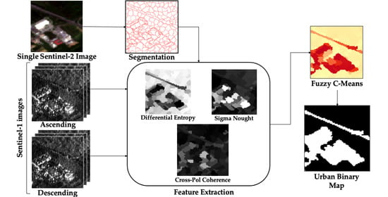
The complete processing chain for the S1–S2 Urban Map (S1S2UM) production is depicted in Figure 5. Combining the two sensor types in this work is complementary: one S2 image is used to identify clusters of similar pixels. For each window, we extract a set of SAR features from an S1 stack. Finally, urban mapping is achieved in the framework of an unsupervised classifier.

2.2.1. Superpixels Segmentation

Superpixels segmentation [38] divides pixels into small, homogeneous, compact, and similarly sized groups. They capture redundancy in the image, up to a certain level of detail. As opposed to other segmentation methods, superpixels do not try to capture the entire object; rather, they almost always result in an over-segmentation.

Simple Linear Iterative Clustering (SLIC) [39] is a popular algorithm out of the superpixels family. It is based on a gradient descent approach, starting from a poor segmentation (usually square), and iteratively relabels the pixels to optimize the objective function. Clusters are generated based on their color similarity and proximity in the image plane. In this work, the MATLAB implementation of the SLIC algorithm was used, which takes as input three color channels.

We applied SLIC superpixels to an S2 optical image, exploiting the algorithm’s ability to generate segments that follow shapes in the image, yet are relatively homogeneous in size. The latter guarantees that a similar number of pixels are used to compute SAR-based features, which is important for handling noise and bias in coherence estimation.

Three parameters can tune the performance: Initial spatial interval between segments (S), compactness (m), and the choice of S2 bands. The first two control the shape of the segment, while the latter relates to the ability to distinguish between objects. Calibration of the parameters was performed to analyze the maximal achievable accuracy using a test site around Lainate, Italy. For each tested configuration, we determine the label of a segment by the mode label of its pixels, according to the ground truth data (DUSAF-6). The resulting accuracy simulates the performance of an ideal classifier. An evaluation of the accuracy for different values of the spatial interval and the compactness is shown in Figure 6. Values of S = 70 m and m = 20 were chosen as a trade-off between segment size and accuracy. The choice of S2 bands is based on empirical experiments, which showed superior performance using the Green-Blue-NIR high-resolution channels.

Finally, an example of the segmentation results is shown in Figure 7. It is noticeable how detailed features, such as roads, are preserved, while coarse segments are sufficient to describe continues surfaces, such as fields.

2.2.2. Projection to Range-Azimuth

The joint exploitation of the optical segment map and the SAR stack requires moving to a common coordinate system.

Geocoding is the transformation between coordinates of the imaging system (range-azimuth) and orthonormal map coordinates [40]. The inverse operation, transforming map coordinates into SAR coordinates, is known as forward-geocoding. For each pixel in the range-azimuth domain, a corresponding position in the map projection is computed.

After performing the optical image segmentation, a map of indexes defines the relation between pixels and segments. We project the map into the range-azimuth domain (defined by the master image of the SAR stack). One can achieve the projection by forward-geocoding or by interpolation of the geocoding indexes.

We performed the segmentation in the S2 native resolution (10 m) and only then projected the segment map to the grid defined by the SAR acquisition (2.3 m × 14.1 m). The result is a Look-Up Table (LUT), mapping between segment index in the geocoded domain and a set of indices in the SAR geometry. The operation allows achieving maximal segmentation accuracy while performing SAR feature estimation without prior multi-looking and resampling. Since both ascending and descending acquisitions are utilized, the process is repeated for each geometry.

Notice that once the segments in the range-azimuth domain are classified, no further geocoding is required. The transformation to latitude–longitude is easily achieved by inverting the LUT.

2.2.3. SAR Features Extraction

Three SAR-based features were discussed in Section 2.1: differential entropy, sigma-nought, and polarimetric coherence. Instead of using a boxcar window, the features are computed for each cluster of pixels identified in the segmentation process.

The advantage of an OBIA approach is in the preservation of the scene’s details since the averaging window is determined by an optical image that is not affected by speckle. The result is demonstrated in Figure 8, where the shapes of buildings and roads are well distinguishable.

SAR data contain inherent geometric distortions, i.e., layover and shadow effects, which can impact the ability to capture a given LC accurately. Additionally, human-made targets tend to be oriented and distributed randomely, affecting the double bounce effect detection. Having two stacks, taken from different orbit directions (i.e., ascending and descending), provides two lines of sight and can help mitigate the problem.

2.2.4. Classifier

Fuzzy C-Mean (FCM) [41] is an unsupervised process for grouping a dataset in c clusters in a way that maximizes the similarity between data within a cluster, accounting for the fact that boundaries between natural classes may be overlapping. The algorithm randomly initializes a set of c centroids and iteratively updates a membership matrix, describing the degree of association of the ith sample to the jth cluster. The procedure minimizes the following objective function:

$$J={\displaystyle \sum }_{j=1}^c{\displaystyle \sum }_{i=1}^N{\mu }_{ij}{d}_{ij} ,$$

(10)

where N is the total number of samples, $d_{ij}$ is the euclidian distance between a sample and the centroid. The membership function is computed according to:

$${\mu }_{ij}=\frac{1}{{{\displaystyle \sum }}_{k=1}^c{\left(\frac{d_{ij}}{d_{ik}}\right)}^{\frac{2}{m-1}}} ,$$

(11)

being m a scalar (m > 1), which controls the fuzziness of the resulting clusters. m = 2 was suggested as an optimal value [42] when no prior knowledge is available and was adopted in this work.

FCM is widely used for geospatial problems [43,44] due to the overlapping nature of remote-sensing data. A soft classification approach allows to perform further post-processing and to highlight different aspects in the final result. The fact that no training data are required is of great interest for land cover applications, as reliable ground truth data are usually unavailable.

In the context of this work, a fuzzy approach was selected as appropriate due to the limits of resolution of both S1 and S2 sensors. The segmentation of the optical image was tuned to obtain segments that are large enough to facilitate robust estimation of SAR features. While the majority of pixels in a segment are expected to belong to the same land cover type, some mixture is inevitable. Fuzzy logic allows postponing the hard thresholding to a later stage, which might be application dependant.

FCM with two clusters was used (c = 2). Since the eucleadian distance is computed as a measure of similarity, the features must be provided at a common scale. We used all features to have a zero median and interquartile range of one.

Minimal ground truth is needed for class identification, i.e., correctly relating the membership score to the urban/non-urban class. We used as before that the urban class is the minority label in the sites we tested.

3. Case Studies

This section demonstrates the generation of urban LC maps using the S1S2UM workflow. Preliminary results are provided for a site around Lainate, Italy, showing the effectiveness of S1S2UM to accurately delineate the boundaries between land covers. Further assessment of performance was performed over two sites in Portugal, comparing the results with published datasets.

3.1. Lainate, Italy

The generation of the urban extent for a 13 km × 11 km site around Lainate (north Italy) is shown in this section (see Figure 9). Two stacks of 8 Sentinel-1 IW images were retrieved from ascending and descending orbits (see

Table 1. Remote sensing data used for the Lainate test site.

Site	Sentinel-1 Ascending	Sentinel-1 Descending	Sentinel-2
Lainate	11-04-2018	30-04-2018	22-04-2018
	17-04-2018	06-05-2018
	23-04-2018	12-05-2018
	29-04-2018	18-05-2018
	05-05-2018	24-05-2018
	11-05-2018	30-05-2018
	17-05-2018	05-06-2018
	23-05-2018	11-06-2018

). Each stack is coregistered to its unique master. Furthermore, a cloudless optical image is needed for segmentation purposes. We used an S2 level 2A image with low reported cloud coverage (<2%), and no further cloud masking was performed.

The fuzzy classification results are shown in Figure 9, where buildings are clearly marked by high membership values. As expected, forests and agriculture areas are denoted by low levels of membership values. The unsupervised classifier results in moderate to low values for some roads and concrete surfaces, which will be discussed in Section 4. Detailed examples of the classification are provided in Figure 10. The outlines of building clusters are well portraited by S1S2UM as a consequence of the superpixels segmentation.

3.2. Braga and Coimbra, Portugal

Two sites in Portugal are used for performance evaluation. The areas are located around the cities of Braga and Coimbra (see Figure 11) and were chosen since they exhibit diverse types of land covers, such as cities, sparse villages, agriculture fields, and bare soil. The presence of complex topography causes distortions in geometry and amplitude of the acquired image, which need to be treated carefully to obtain correct results. The two datasets are reported

Table 2. Remote sensing data used for Portugal test sites.

Site	Sentinel-1 Ascending	Sentinel-1 Descending	Sentinel-2
Braga	02-05-2017	01-05-2017	28-04-2017
	08-05-2017	07-05-2017
	14-05-2017	13-05-2017
	20-05-2017	19-05-2017
	26-05-2017	25-05-2017
	01-06-2017	31-05-2017
	07-06-2017	06-06-2017
	13-06-2017	12-06-2017
Coimbra	27-03-2017	20-04-2017	04-06-2017
	02-04-2017	26-03-2017
	08-04-2017	01-04-2017
	14-04-2017	07-04-2017
	20-04-2017	13-04-2017
	26-04-2017	19-04-2017
	02-05-2017	25-04-2017
	08-05-2017	01-05-2017

.

Figure 12 shows the results of the Fuzzy classification of urban areas using the proposed fusion of SAR and optical data. The color denotes the degree of membership of each pixel to the urban class.

In the absence of a reliable ground truth layer, the results are compared with two state-of-the-art single-source approaches that exclusively use one type of sensor: Sentinel-2 Global Land Cover (S2GLC) and Global Urban Footprint (GUF).

S2GLC is a 10 m LC map for the year 2017 over Europe, generated using S2 data only [45]. It is published on the CREODIAS platform, and the relevant tile was downloaded for the sake of the analysis presented here. The method is based on pixel-wise random forest classification and requires nineteen cloudless images for a given area, collected over an entire year. In some cases, it is reported that weather conditions are too harsh, and the selection criteria could not be met. The published map contains thirteen land cover types made possible by the multi-spectral capabilities of S2. The authors used existing datasets with lower resolutions (20 m) for training and testing and achieved 86.1% Overall Accuracy (OA) on a continental scale.

GUF is a binary settlement map derived from high-resolution SAR missions [46]. It is globally available by request from the German Aerospace Center (DLR). A stack of TanDEM-X and TerraSAR-X X-band images (3 m resolution) from 2011 to 2012 was utilized to classify amplitude and speckle divergence, where pixels exhibiting high values for both features were denoted as urban. Post-processing was performed with reference layers for false alarm removal and threshold tunning, with a reported OA of around 85%. The final result was published in a 12 m resolution, and we resampled it to match the 10 m grid of S2.

In order to obtain a binary urban map, the fuzzy membership values were thresholded, with an empirical threshold of 0.6. However, the value might be application dependant and can be tuned using existing low-resolution ground truth. A statistical comparison between S1S2UM and the two reference works is provided in the form of a confusion matrix (

Table 3. Portugal classification confusion matrix and quantitative analysis.

	Predicted	S2GLC		GUF
		urban	non-urban	urban	non-urban
Coimbra	urban	431759	249052	521543	159268
	non-urban	307615	10049594	524730	9832479
	OA	94.96%		93.80%
	K-coefficient	58.11%		57.20%
Braga	urban	954600	428575	1060100	323075
	non-urban	510838	7541182	851409	7200611
	OA	90.04%		87.5%
	K-coefficient	61.16%		57.05%

), reporting the agreements between the methods on a pixel level. A visual demonstration of the differences between the approaches is given in Figure 13.

3.3. Updating Urban LC Maps

Many techniques were developed to generate accurate urban land cover maps; however, they usually require a long sensing period and complex processing. Thus, published maps are usually available at a given time instance. Many areas of the world exhibit rapid growth, raising the need to generate frequent updates to LC maps.

An additional dataset was collected for the Braga test site from the spring of 2020 to illustrate the applicability of S1S2UM for the delineation of new urban targets. The qualitative changes between the periods can be appreciated in Figure 14.

4. Discussion

Looking at Figure 12, it is visible that the urban centers are well highlighted by high membership values. Due to the fuzzy nature of the classification, it is noticeable that areas covered by bare soil exhibit moderate membership levels, due to their high coherence (see right side of Figure 12c). Nevertheless, the values are well distinguished from those of real urban targets, and thus a threshold can be applied to exclude them.

The comparison between S1S2UM and S2GLC suggests a significant statistical correlation (average K-coefficient of around 60%) between the two methods. However, some differences are noticeable and can be appreciated from Figure 13a,c. S2GLC was generated in a pixel-wise fashion and so is theoretically able to detect very small targets (10 m). On the contrary, S1S2UM is an object-based approach that limits the size of the smallest detail. Since SAR data are used for the thematic interpretation, object size was kept relatively large to avoid coherent estimation over a small number of looks, which is prone to bias.

The SAR features of S1S2UM are tuned to detect high concentrations of permanent scatterers and stable targets. Roads are narrow surfaces without any double-bounce scattering mechanisms (usually) and are surrounded by decorrelating targets, causing difficulties in their classification. S2GLC uses spectral signatures and is superior in terms of road identification.

A sizable discrepancy is visible in the left side of Figure 13c, where a large red area suggests a missed detection. However, a visual check was performed, and agriculture fields cover the zone, so S1S2UM is correct as labeling the site as non-urban. In general, manual inspection suggests that the two maps provide complementary information in many cases, and the actual precision/recall might be higher than reported. Thanks to the object-based approach, the coarser resolution of the SAR sensor (20 m × 5 m) is sufficient to provide a result comparable to the S2 LC, which is processed with a 10 m resolution. The result is especially impressive considering the long sensing period required by S2GLC (around a year), compared to less than two months for the method suggested here.

Regarding the comparison with GUF, both methods are SAR-based, thus suffering from similar problems related to the need of spatial/temporal averaging. However, lower accuracies and K-coefficients were noted with respect to the comparison with S2GLC. Observing Figure 13b,d it appears that GUF tends to overfit urban areas, extending their edges further than needed. Perhaps the effect is the result of the texture analysis or the post-processing steps. In this work, we used data from 2017, while GUF is updated to 2012. Thus, it is reasonable that some new targets are recognized only by S1S2UM (clusters of blue pixels), decreasing the actual precision.

The qualitative examples in Figure 14 demonstrate the ability to generate up-to-date urban maps. The border between the urban and non-urban land covers is clearly extended in 2020 to include the new buildings. Many changes are not easily interpretable due to the limited pixel size of S2 and should be investigated with high-resolution data. The task is left to be performed in further work.

5. Conclusions

In this paper, we exploit the potential of combining SAR and MS data in the context of an OBIA classification for urban map generation. A simple processing chain was established, gaining from the difference in the nature of the two data sources. The geometric segment definition is obtained from an optical image with the help of superpixels which are robust, effective, and easy to employ. The physical characteristics of targets are deduced from a set of SAR features selected for their efficiency over short stacks. Three features were found that were enough to obtain promising results: differential entropy, sigma nought, and polarimetric coherence. An unsupervised FCM classifier is then employed to translate the features into urban membership level. The result is thresholded to obtain binary classification.

Efficiency is gained by exploiting superpixels to reduce the number of samples from pixels to segments. Additionally, the selected set of features are very simple for computation; innovative utilization of the differential entropy allows a robust quantification of the level of stability, with the low cost of calculating a determinant of an N × N matrix (being N the number of SAR images used for the processing). The simple implementation and the short sensing period can allow users to produce urban maps regularly, tracking changes in developing regions.

S1S2UM requires only one MS image over the entire period, which strongly minimizes limitations related to cloud coverage and unfavorable weather. Illumination conditions are also not a significant concern of this technique, as the MS bands are used for segmentation only.

Obtaining suitable high-resolution labeled data is unfeasible in most parts of the world. The unsupervised classification fashion chosen for this work means no training dataset is used, making the proposed solution applicable worldwide.

The methodology was tested with S1 and S2 data over two sites in Portugal. Two reference works were compared, one based on S2 pixels-wise classification, and the other exploits high-resolution SAR sensors and texture analysis. An overall accuracy between 88% and 95% was achieved, also in the presence of irregular topography. The comparison showed significant statistical similarity between the result, especially encouraging due to the much shorter sensing period used in this work. Less than two months of data, with a regular sampling period of six days, are sufficient for the results presented here.

Following this work, further investigation should be performed on the possibility of increasing the number of observed labels. Additionally, improving segmentation by introducing optical images with finer resolution should be better explored. Finally, the processing of large-scale terrains can be established.

References

- De Martinao, M.; Causa, F.; Serpico, S.B. Classification of Optical High Resolution Images in Urban Environment Using Spectral and Textural Information. In Proceedings of the IGARSS 2003—2003 IEEE International Geoscience and Remote Sensing Symposium—Proceedings (IEEE Cat. No.03CH37477), Toulouse, France, 21–25 July 2003; Volume 1, pp. 467–469. [Google Scholar]
- Mendili, L.; Puissant, A.; Chougrad, M.; Sebari, I. Towards a Multi-Temporal Deep Learning Approach for Mapping Urban Fabric Using Sentinel 2 Images. Remote Sens. 2020, 12, 423. [Google Scholar] [CrossRef] [Green Version]
- Yu, L.; Wang, J.; Gong, P. Improving 30 m Global Land-Cover Map FROM-GLC with Time Series MODIS and Auxiliary Data Sets: A Segmentation-Based Approach. Int. J. Remote Sens. 2013, 34, 5851–5867. [Google Scholar] [CrossRef]
- Schug, F.; Frantz, D.; Okujeni, A.; van der Linden, S.; Hostert, P. Mapping Urban-Rural Gradients of Settlements and Vegetation at National Scale Using Sentinel-2 Spectral-Temporal Metrics and Regression-Based Unmixing with Synthetic Training Data. Remote Sens. Environ. 2020, 246, 111810. [Google Scholar] [CrossRef] [PubMed]
- Tison, C.; Nicolas, J.-M.; Tupin, F.; Maitre, H. A New Statistical Model for Markovian Classification of Urban Areas in High-Resolution SAR Images. IEEE Trans. Geosci. Remote Sens. 2004, 42, 2046–2057. [Google Scholar] [CrossRef]
- Chini, M.; Pelich, R.; Hostache, R.; Matgen, P.; Lopez-Martinez, C. Towards a 20 m Global Building Map from Sentinel-1 SAR Data. Remote Sens. 2018, 10, 1833. [Google Scholar] [CrossRef] [Green Version]
- Corr, D.G.; Walker, A.; Benz, U.; Lingenfelder, I.; Rodrigues, A. Classification of Urban SAR Imagery Using Object Oriented Techniques. In Proceedings of the IGARSS 2003—2003 IEEE International Geoscience and Remote Sensing Symposium—Proceedings (IEEE Cat. No.03CH37477), Toulouse, France, 21–25 July 2003; Volume 1, pp. 188–190. [Google Scholar]
- Strozzi, T.; Wegmuller, U. Delimitation of Urban Areas with SAR Interferometry. In Proceedings of the IGARSS ’98. Sensing and Managing the Environment—1998 IEEE International Geoscience and Remote Sensing—Symposium Proceedings. (Cat. No.98CH36174), Seattle, WA, USA, 6–10 July 1998; Volume 3, pp. 1632–1634. [Google Scholar]
- Jacob, A.W.; Vicente-Guijalba, F.; Lopez-Martinez, C.; Lopez-Sanchez, J.M.; Litzinger, M.; Kristen, H.; Mestre-Quereda, A.; Ziółkowski, D.; Lavalle, M.; Notarnicola, C.; et al. Sentinel-1 InSAR Coherence for Land Cover Mapping: A Comparison of Multiple Feature-Based Classifiers. IEEE J. Sel. Top. Appl. Earth Obs. Remote Sens. 2020, 13, 535–552. [Google Scholar] [CrossRef] [Green Version]
- Perissin, D.; Ferretti, A. Urban-Target Recognition by Means of Repeated Spaceborne SAR Images. IEEE Trans. Geosci. Remote Sens. 2007, 45, 4043–4058. [Google Scholar] [CrossRef]
- Koppel, K.; Zalite, K.; Sisas, A.; Voormansik, K.; Praks, J.; Noorma, M. Sentinel-1 for Urban Area Monitoring—Analysing Local-Area Statistics and Interferometric Coherence Methods for Buildings’ Detection. In Proceedings of the 2015 IEEE International Geoscience and Remote Sensing Symposium (IGARSS), Milan, Italy, 26–31 July 2015; pp. 1175–1178. [Google Scholar]
- Blaschke, T. Object Based Image Analysis for Remote Sensing. ISPRS J. Photogramm. Remote Sens. 2010, 65, 2–16. [Google Scholar] [CrossRef] [Green Version]
- Liu, B.; Hu, H.; Wang, H.; Wang, K.; Liu, X.; Yu, W. Superpixel-Based Classification With an Adaptive Number of Classes for Polarimetric SAR Images. IEEE Trans. Geosci. Remote Sens. 2013, 51, 907–924. [Google Scholar] [CrossRef]
- Tso, B.; Mather, P.M. Crop Discrimination Using Multi-Temporal SAR Imagery. Int. J. Remote Sens. 1999, 20, 2443–2460. [Google Scholar] [CrossRef]
- Dey, V.; Zhang, Y.; Zhong, M. A Review on Image Segmentation Techniques with Remote Sensing Perspective. In Proceedings of the ISPRS TC VII Symposium—100 Years ISPRS, Vienna, Austria, 5–7 July 2010. [Google Scholar]
- Gamba, P.; Aldrighi, M. SAR Data Classification of Urban Areas by Means of Segmentation Techniques and Ancillary Optical Data. IEEE J. Sel. Top. Appl. Earth Obs. Remote Sens. 2012, 5, 1140–1148. [Google Scholar] [CrossRef]
- Arisoy, S.; Kayabol, K. Mixture-Based Superpixel Segmentation and Classification of SAR Images. IEEE Geosci. Remote Sens. Lett. 2016, 13, 1721–1725. [Google Scholar] [CrossRef]
- Pohl, C.; Genderen, J.L.V. Review Article Multisensor Image Fusion in Remote Sensing: Concepts, Methods and Applications. Int. J. Remote Sens. 1998, 19, 823–854. [Google Scholar] [CrossRef] [Green Version]
- Amarsaikhan, D.; Blotevogel, H.H.; van Genderen, J.L.; Ganzorig, M.; Gantuya, R.; Nergui, B. Fusing High-Resolution SAR and Optical Imagery for Improved Urban Land Cover Study and Classification. Int. J. Image Data Fusion 2010, 1, 83–97. [Google Scholar] [CrossRef]
- Chureesampant, K.; Susaki, J. Land Cover Classification Using Multi-Temporal SAR Data and Optical Data Fusion with Adaptive Training Sample Selection. In Proceedings of the 2012 IEEE International Geoscience and Remote Sensing Symposium, Munich, Germany, 22–27 July 2012; pp. 6177–6180. [Google Scholar]
- Gomez-Chova, L.; Fernández-Prieto, D.; Calpe, J.; Soria, E.; Vila, J.; Camps-Valls, G. Urban Monitoring Using Multi-Temporal SAR and Multi-Spectral Data. Pattern Recognit. Lett. 2006, 27, 234–243. [Google Scholar] [CrossRef]
- Ban, Y.; Hu, H.; Rangel, I.M. Fusion of Quickbird MS and RADARSAT SAR Data for Urban Land-Cover Mapping: Object-Based and Knowledge-Based Approach. Int. J. Remote Sens. 2010, 31, 1391–1410. [Google Scholar] [CrossRef]
- Waske, B.; van der Linden, S. Classifying Multilevel Imagery From SAR and Optical Sensors by Decision Fusion. IEEE Trans. Geosci. Remote Sens. 2008, 46, 1457–1466. [Google Scholar] [CrossRef]
- Clerici, N.; Calderón, C.A.V.; Posada, J.M. Fusion of Sentinel-1A and Sentinel-2A Data for Land Cover Mapping: A Case Study in the Lower Magdalena Region, Colombia. J. Maps 2017, 13, 718–726. [Google Scholar] [CrossRef] [Green Version]
- Blaes, X.; Vanhalle, L.; Defourny, P. Efficiency of Crop Identification Based on Optical and SAR Image Time Series. Remote Sens. Environ. 2005, 96, 352–365. [Google Scholar] [CrossRef]
- Santoro, M.; Fanelli, A.; Askne, J.; Murino, P. Monitoring Urban Areas by Means of Coherence Levels. In Proceedings of the Second International Workshop on ERS SAR Interferometry, Liège, Belgium, 10–12 November 1999. [Google Scholar]
- Pulvirenti, L.; Chini, M.; Pierdicca, N.; Boni, G. Use of SAR Data for Detecting Floodwater in Urban and Agricultural Areas: The Role of the Interferometric Coherence. IEEE Trans. Geosci. Remote Sens. 2016, 54, 1532–1544. [Google Scholar] [CrossRef]
- Rocca, F. Modeling Interferogram Stacks. IEEE Trans. Geosci. Remote Sens. 2007, 45, 3289–3299. [Google Scholar] [CrossRef]
- Parizzi, A.; Cong, X.; Eineder, M. First Results from Multifrequency Interferometry. A Comparison of Different Decorrelation Time Constants at L, C, and X Band. In Proceedings of the ESA Scientific Publications, Frascati, Italy, December 2009; pp. 1–5. [Google Scholar]
- Tang, P.; Zhou, W.; Tian, B.; Chen, F.; Li, Z.; Li, G. Quantification of Temporal Decorrelation in X-, C-, and L-Band Interferometry for the Permafrost Region of the Qinghai–Tibet Plateau. IEEE Geosci. Remote Sens. Lett. 2017, 14, 2285–2289. [Google Scholar] [CrossRef]
- Sica, F.; Pulella, A.; Nannini, M.; Pinheiro, M.; Rizzoli, P. Repeat-Pass SAR Interferometry for Land Cover Classification: A Methodology Using Sentinel-1 Short-Time-Series. Remote Sens. Environ. 2019, 232, 111277. [Google Scholar] [CrossRef]
- Monti-Guarnieri, A.; Manzoni, M.; Giudici, D.; Recchia, A.; Tebaldini, S. Vegetated Target Decorrelation in SAR and Interferometry: Models, Simulation, and Performance Evaluation. Remote Sens. 2020, 12, 2545. [Google Scholar] [CrossRef]
- Jiang, M.; Hooper, A.; Tian, X.; Xu, J.; Chen, S.-N.; Ma, Z.-F.; Cheng, X. Delineation of Built-up Land Change from SAR Stack by Analysing the Coefficient of Variation. ISPRS J. Photogramm. Remote Sens. 2020, 169, 93–108. [Google Scholar] [CrossRef]
- Small, D. Flattening Gamma: Radiometric Terrain Correction for SAR Imagery. IEEE Trans. Geosci. Remote Sens. 2011, 49, 3081–3093. [Google Scholar] [CrossRef]
- Jong-Sen, L.; Hoppel, K.W.; Mango, S.A.; Miller, A.R. Intensity and Phase Statistics of Multilook Polarimetric and Interferometric SAR Imagery. IEEE Trans. Geosci. Remote Sens. 1994, 32, 1017–1028. [Google Scholar] [CrossRef]
- Prati, C.M.; Rocca, F.; Asaro, F.; Belletti, B.; Bizzi, S. Use of Cross-POL Multi-Temporal SAR Data for Image Segmentation. In Proceedings of the 2018 IEEE International Conference on Environmental Engineering (EE), Milan, Italy, 12–14 March 2018; pp. 1–6. [Google Scholar]
- Atwood, D.K.; Thirion-Lefevre, L. Polarimetric Phase and Implications for Urban Classification. IEEE Trans. Geosci. Remote Sens. 2018, 56, 1278–1289. [Google Scholar] [CrossRef]
- Wang, M.; Liu, X.; Gao, Y.; Ma, X.; Soomro, N.Q. Superpixel Segmentation: A Benchmark. Signal Process. Image Commun. 2017, 56, 28–39. [Google Scholar] [CrossRef]
- Achanta, R.; Shaji, A.; Smith, K.; Lucchi, A.; Fua, P.; Süsstrunk, S. SLIC Superpixels Compared to State-of-the-Art Superpixel Methods. IEEE Trans. Pattern Anal. Mach. Intell. 2012, 34, 2274–2282. [Google Scholar] [CrossRef] [PubMed] [Green Version]
- Bamler, R.; Schättler, B. SAR Geocoding: Data and Systems; Schreier, G., Ed.; Wichman: Karlsruhe, Germany, 1993; pp. 53–102. [Google Scholar]
- Bezdek, J.C.; Ehrlich, R.; Full, W. FCM: The Fuzzy c-Means Clustering Algorithm. Comput. Geosci. 1984, 10, 191–203. [Google Scholar] [CrossRef]
- Shen, Y.; Shi, H.; Zhang, J.Q. Improvement and Optimization of a Fuzzy C-Means Clustering Algorithm. In Proceedings of the 18th IEEE Instrumentation and Measurement Technology Conference. Rediscovering Measurement in the Age of Informatics (Cat. No.01CH 37188), Budapest, Hungary, 21–26 May 2001; Volume 3, pp. 1430–1433. [Google Scholar]
- Burrough, P.A.; van Gaans, P.F.M.; MacMillan, R.A. High-Resolution Landform Classification Using Fuzzy k-Means. Fuzzy Sets Syst. 2000, 113, 37–52. [Google Scholar] [CrossRef]
- Corbane, C.; Jean-François, F.; Baghdadi, N.; Villeneuve, N.; Petit, M. Rapid Urban Mapping Using SAR/Optical Imagery Synergy. Sensors 2008, 8, 7125–7143. [Google Scholar] [CrossRef]
- Malinowski, R.; Lewiński, S.; Rybicki, M.; Gromny, E.; Jenerowicz, M.; Krupiński, M.; Nowakowski, A.; Wojtkowski, C.; Krupiński, M.; Krätzschmar, E.; et al. Automated Production of a Land Cover/Use Map of Europe Based on Sentinel-2 Imagery. Remote Sens. 2020, 12, 3523. [Google Scholar] [CrossRef]
- Esch, T.; Heldens, W.; Hirner, A.; Keil, M.; Marconcini, M.; Roth, A.; Zeidler, J.; Dech, S.; Strano, E. Breaking New Ground in Mapping Human Settlements from Space—The Global Urban Footprint. ISPRS J. Photogramm. Remote Sens. 2017, 134, 30–42. [Google Scholar] [CrossRef] [Green Version]
Figure 1.
Estimated coherence matrix: (a) Exponential decorrelation characterized by a decay time of 24 days. (b) PS with constant coherence of 0.8.
Figure 2.
Differential entropy probability density estimation. Computed for a stack of 8 SAR images with 6 days temporal baseline over Lainate, Italy. A spatial window of 25 × 5 samples was used.
Figure 3.
Sigma nought probability density estimation for Lainate, Italy.
Figure 4.
Cross-pol coherence probability density estimation for Lainate, Italy.
Figure 5.
Flow chart of the proposed algorithm for urban mapping.
Figure 6.
Segmentation accuracy as function of the two parameters to be tuned: compactness (m) and spatial interval (S).
Figure 7.
Superpixels segmentation, demonstrated in a 4 km × 3 km site in Lainate, Italy. (a) S2 RGB reference (b) Average RGB values for the segmented image.
Figure 8.
SAR features example, using the segmentation scheme. (a) S2 reference image (b) Differential entropy (c) Sigma naught (d) Polarimetric Coherence.
Figure 9.
Lainate (north Italy) 13 km × 11 km test site. (a) Sentinel-2 RGB image. (b) FCM classification results. The color scale quantifies the level of membership to the urban class. Note that the value is continoues in the range (0,1) where red: urban, yellow: non-urban.
Figure 10.
Lainate classification results, demonstrated for 2 km × 2 km sections. (a,c,e): S2 reference. (b,d,f): S1S2UM fuzzy classification result, where red: urban pixels, yellow: non-urban pixels.
Figure 11.
Portugal test sites. (a) Used polygons around the cities of Braga (top rectangle) and Coimbra (bottom rectangle) with a Google Earth background. (b) S2 image of the Braga site. (c) S2 image of the Coimbra site.
Figure 12.
FCM classification results for Braga (a) and Coimbra (c). Color scale quantifies the membership level of each segment to the urban class, where red: urban pixels, yellow: non-urban pixels. (b,d): S2GLC reference binary map where white: urban pixels, black: non-urban pixels.
Figure 13.
Comparison with state-of-the-art techniques for Coimbra (a,b) and Braga (c,d). Green: pixels detected as urban by S1S2UM and the reference methods, S2GLC (a,c) and GUF (b,d). Blue: pixels detected only by S1S2UM. Red: pixels detected only by the reference method.
Figure 14.
Examples of urban areas borders for two different periods (left: 2017, right: 2020).