Mid-Term Monitoring of Glacier’s Variations with UAVs: The Example of the Belvedere Glacier

Abstract

Recently, Unmanned Aerial Vehicles (UAV) have opened up unparalleled opportunities for alpine glacier monitoring, as they allow for reconstructing extensive and high-resolution 3D models. In order to evaluate annual ice flow velocities and volume variations, six yearly measurements were carried out between 2015 and 2020 on the debris-covered Belvedere Glacier (Anzasca Valley, Italian Alps) with low-cost fixed-wing UAVs and quadcopters. Every year, ground control points and check points were measured with GNSS. Images acquired from UAV were processed with Structure-from-Motion and Multi-View Stereo algorithms to build photogrammetric models, orthophotos and digital surface models, with decimetric accuracy. Annual glacier velocities were derived by combining manually-tracked features on orthophotos with GNSS measurements. Velocities ranging between 17 m y⁻¹ and 22 m y⁻¹ were found in the central part of the glacier, whereas values between 2 m y⁻¹ and 7 m y⁻¹ were found in the accumulation area and at the glacier terminus. Between 2 × 10⁶ m³ and 3.5 × 10⁶ m³ of ice volume were lost every year. A pair of intra-year measurements (October 2017–July 2018) highlighted that winter and spring volume reduction was ∼1/4 of the average annual ice loss. The Belvedere monitoring activity proved that decimetric-accurate glacier models can be derived with low-cost UAVs and photogrammetry, limiting in-situ operations. Moreover, UAVs require minimal data acquisition costs and allow for great surveying flexibility, compared to traditional techniques. Information about annual flow velocities and ice volume variations of the Belvedere Glacier may have great value for further understanding glacier dynamics, compute mass balances, or it might be used as input for glacier flow modelling.

1. Introduction

Glaciers all over the world are experiencing a rapid retreat caused by climate change [1,2]. In particular, many alpine glaciers, located in temperate areas, are suffering from increasing temperature [3,4]. Projections point out that European Alps may lose more than 60% of ice volume by the end of the century under RCP2.6 scenario, whereas a larger amount of ice loss is expected under worse scenarios [5]. As a consequence, alpine glaciers are widely considered as a proxy for climate change evaluation, and the number of studies concerning glaciers has soared in the past few years.

Traditional glacier monitoring techniques usually involve repeated in-situ measurements at stakes and snow pits, properly distributed over the glacier, to quantify ice height variation and estimate annual mass balance [2]. These might be integrated with geodetic GNSS and photogrammetric techniques in order to accurately determine morphological changes on the glacier surface and compute volume variations (e.g., [6,7,8]). Direct in-situ techniques, however, are likely time consuming and often requires mountaineering expertise, as glacial environments are often dangerous.

Thanks to the global coverage, the long time-series of data available and the short revisiting period, satellite optical imageries are nowadays widely used to derive planimetric glacier displacements and ice flow velocities [9,10,11,12,13]. Satellite SAR data can be used to measure 3D motion of glaciers [14,15,16]. More recently, 3D glacier modelling by means of satellite optical stereo pairs have been explored (e.g., [17,18]). Nevertheless, satellite imagery resolution might be still rather coarse for small alpine glaciers monitoring, if accurate volume variations or velocity fields are needed.

In the past 10 years, Unmanned Aerial Vehicles (UAVs) have experienced a rapid technological development and cost reduction, and they are nowadays considered as valuable tools for environmental monitoring. Thanks to Structure-from-Motion photogrammetry (SfM) [19] and Multi-View Stereo (MVS) [20] algorithms, images taken by cameras on-board UAVs can be used to build high resolution 3D point clouds, Digital Surface Models (DSMs) and orthophotos. UAVs have been employed for applications such as geomorphology modelling [21,22], river flow velocity and discharge estimation [23,24], snow volume calculation [25,26,27], dam sediment volume evaluation [28].

Moreover, several examples of UAVs and photogrammetry for cryosphere monitoring can be found in the literature [29]. Reference [30] employed a fixed-wing UAV and a remotely-piloted helicopter, carrying low-cost compact cameras, to generate orthophotos and DSMs of the Fountain Glacier in the Canadian Arctic. References [31,32] used a fixed-wing UAV to evaluate seasonal surface velocities of the debris-covered Lirung Glacier, in Nepal. They succeeded in deriving surface velocities from orthophotos by phase correlation, and they found summer velocities to be almost double than those occurred in wintertime. Reference [33] evaluated the influence of the number and disposition of Ground Control Points (GCPs) on the accuracy of glacier DSMs derived from UAVs.

The rising number of recent works [34,35,36] highlights the potential of UAVs and low-cost photogrammetry to efficiently monitor small and mid-scale glaciers with high spatial resolution. In fact, UAVs allows for extensively reconstruct glaciers morphology (e.g., with DSMs and orthophotos) with limited in-situ operations and costs [29]. This would not be possible with traditional stake measurements, as they can only provide sparse information to be interpolated over the whole glacier and they are usually more time consuming.

Among alpine glaciers, the Belvedere Glacier (Macugnaga, VCO – Italian Alps) is of particular relevance because it reaches low altitude (about 1800 m a.s.l.) and it is a debris-covered glacier. This helped to protect the ice from solar radiation, and limited ice volume reduction due to the increasing air temperature [6,37]. Moreover, over the past century, the Belvedere Glacier experienced extraordinary dynamics, such as a surge-type movement or the formation of a supra-glacial lake, which seriously threatened the nearby municipality of Macugnaga [10,38]. Due to its particular relevance, the Belvedere Glacier has been widely studied for decades [6,18,37,38,39,40,41,42,43] and it is still object of monitoring by local authorities. Nevertheless, at the best of authors knowledge, there are no recent works aimed at continuously monitor the glacier dynamics for a period of several years with a high geometrical resolution and accuracy. With this work, we want to fill this gap and present the results of a 6-years-long monitoring activity, which allowed us to accurately document Belvedere Glacier geomorphological variations, by employing geomatics techniques. This piece of information may be crucial for further glaciological analysis.

Between 2015 and 2020, an extensive and continuous monitoring activity aimed at investigating the annual evolution of the Belvedere Glacier was carried out with UAVs-based photogrammetry and in-situ GNSS measurements. The monitoring activity was designed and conducted jointly by the Department of Civil and Environmental Engineering (DICA) of Politecnico di Milano and the Department of Environment, Land and Infrastructure Engineering (DIATI) of Politecnico di Torino. Moreover, the DREAM projects (DRone tEchnnology for wAter resources and hydrologic hazard Monitoring), involving teachers and students from Alta Scuola Politecnica (ASP) of Politecnico di Torino and Milano, contributed to the campaign from 2015 to 2017. Every year, fixed-wing UAVs and quadcopters were used to remotely sense the glacier and build high-resolution photogrammetric models in order to estimate annual variations of ice volume and ice flow velocities. This information, retrieved with geomatics techniques, may be crucial for glaciologists to understand glacier flow dynamics and compute hydrological mass balances, and it also might be used as input of kinematics glacier flow models.

The aim of this work is twofold:

1.

Document yearly changes of the Belvedere Glacier in terms of volume variations and ice flow velocity during the timespan 2015–2020 by using UAV-based photogrammetry and geomatics techniques;

2.

Prove the effectiveness of low-cost UAV-based photogrammetry for periodical alpine glacier monitoring with high geometrical accuracy (i.e., decimetric).

2. Area of Study

The Belvedere Glacier is a temperate alpine glacier located on the east face of Monte Rosa, the Anzasca Valley, Italy. It extends from an altitude of about ∼2250 m a.s.l and reaches its lowest altitude at about 1800 m a.s.l., where it splits in two different glacier tongues (Figure 1a). The Belvedere Glacier covers an area of $\sim 1.8$ $\mathrm{k}$$\mathrm{m}$${}^2$ and it is mainly elongated in South-North direction, with a length of $\sim 3000$ $\mathrm{m}$ and a maximum width of only $\sim 500$ $\mathrm{m}$. Similarly to Miage glacier (Monte Bianco, Valle d’Aosta), the Belvedere Glacier is almost completely covered by rocks and debris. Due to the global warming trend, the number of black glaciers along the Italian Alps is rising [37]. Up to the beginning of the century, the debris cover helped to compensate the effect of the increased temperature, establishing a negative feedback in the temperature-ablation relationship [6,37]. However, in recent years, the debris cover protection has not been sufficient to limit the glacier retreat.

From the morphological point of view, the Belvedere Glacier can be roughly divided into three sectors:

1.

Upper sector (labelled as S1 in Figure 1a): it consists in the accumulation zone. It is located at about 2250 m a.s.l., at the feet of the steep Monte Rosa and the North Locce Glaciers, from which recurrent ice and snow avalanches feed the Belvedere Glacier. This sector is also the main deposition area for rocks and debris [37,44];

2.

Central sector (S2 in Figure 1a): it is the transfer zone and it is enclosed by two sinuous moraines. It starts from an altitude of ∼2250 m a.s.l. and it extends downwards for $\sim 1500$ $\mathrm{m}$. This sector shows the highest ice flow velocities and the most irregular surfaces, with the presence of several crevasses;

3.

Lower sector (S3 in Figure 1a): it is the low relief sector. Here, in proximity of the Belvedere hill, the glacier splits in two different tongues: the north-west tongue is the largest and it reaches the lowest altitude of about 1800 m a.s.l. From the north-west tongue, the Anza River springs. A smaller tongue extends from the Belvedere hill towards East and reaches an altitude of about 1850 m a.s.l.

In the past, several floods and slope instabilities originated from particular glacier dynamics threatened the nearby village of Macugnaga and the Mountain Hut Zamboni Zappa, at 2070 m a.s.l., near the glacier moraine [41]. At the beginning of the 21st century, the Belvedere Glacier experienced an extraordinary and particularly relevant surge-type movement [38]. During the late 1990s, the surface speeds of the whole glacier were ranging between 30 m y⁻¹ and 45 $\mathrm{m}$ $\mathrm{y}$⁻¹ [6,10]. During 2000–2001 an accelerated flow in the Monte-Rosa Glacier produced a wave of compression-decompression stresses and strains in the Belvedere Glacier. Surface velocities soared: values up to 200 $\mathrm{m}$ $\mathrm{y}$⁻¹ were observed photogrammetrically during autumn 2001 [41]. The ice thickness increased more than 20 $\mathrm{m}$ and the wave travelled downwards, creating a depression area in the accumulation zone, that was filled by a super-glacial lake, the Lago Effimero [38,45].

3. UAV-Based Monitoring Campaign on Belvedere Glacier

From 2015 to 2020, the Belvedere Glacier was surveyed with cameras mounted on-board UAVs to build a photogrammetric models of the whole glacier with SfM-MVS techniques. From models, DSM and orthophotos were derived enabling the computation of volumes variation and surface velocities.

3.1. Instruments and Surveys Setup

Because of the long duration of the monitoring campaign, the challenging environment and the fact that more than one research group was involved in the project, different UAV platforms and cameras were used. As reported in

Table 1. Summary of the characteristics of the surveys.

Year	Date	UAV	Camera	GSD	GCP	CP
				[m/px]	[#]	[#]
2015	A. 8.10	SenseFly eBee	Canon PowerShot S110	0.07	24	11
	B. 23.10
2016	20.10	SenseFly eBee	Canon PowerShot S110	0.09	31	15
2017	A. 5.10	A. SenseFly eBee	A. Canon PowerShot S110	0.06	27	8
	B. 15.11	B. SenseFly eBee Plus	B. SenseFly S.O.D.A
	C. 16.11	C. DJI Phantom 4 Pro	C. DJI FC6310
2018	23–25.07	Parrot Disco	Hawkeye Firefly 8S	0.05	27	13
2019	29.07–2.08	Parrot Disco	Hawkeye Firefly 8S	0.06	26	10
2020	A. 26–27.07	A. Parrot Disco	A. Hawkeye Firefly 8S	0.05	29	12
	B. 9.08	B. DJI Phantom 4 Pro	B. DJI FC6310

, in 2015 and 2016, a ready-to-fly fixed-wing UAV SenseFly eBee, equipped with a compact camera Canon PowerShot S110, was employed to survey the whole glacier. During 2017, different combinations of UAVs (fixed-wing and quadcopters) and cameras were employed (Table 1). From 2018 to 2020, a low-cost recreational fixed-wing UAV Parrot Disco FPV, with a wingspan of $1.15$ $\mathrm{m}$ and a weight of 750 $\mathrm{g}$, was adapted to carry a small and lightweight action cam Hawkeye Firefly 8S. For each camera, the main sensor and objective characteristics are listed

Table 2. Summary of the characteristics of the cameras employed.

	Canon PowerShot	SenseFly	DJI FC6310	Hawkeye
	S110	S.O.D.A		Firefly 8S
Sensor	1/1.7${}^{″}$ CMOS	1${}^{″}$ CCD	1${}^{″}$ CMOS	1/2.3${}^{″}$ CMOS
Sensor Size [$\mathrm{m}$$\mathrm{m}$${}^2$]	$7.44\times 5.58$	$13.2\times 8.8$	$13.2\times 8.8$	$6.17\times 4.56$
Focal length [$\mathrm{m}$$\mathrm{m}$]	5.2	10.6	8.8	3.8
Image size [$\mathrm{px}$]	$4000\times 3000$	$5472\times 3648$	$5472\times 3648$	$5472\times 3648$
Pixel size [$\mathsf{\mu }$$\mathrm{m}$]	1.9	2.4	2.4	1.34

.

A set of GCPs was materialized with square cross targets, printed on polypropylene sheets and anchored on big rocks (Figure 2b). About 25 targets were deployed over the glacier (named hereafter as moving targets or M# in Figure 2a) and 24 targets (labelled as stable targets or S# in Figure 2a) were placed on stable areas along the moraines so that they were not subjected neither to the ice flow nor to rock falls. Every year, the condition of each target was checked and, if one was damaged or destroyed, the polypropylene sheet was replaced by keeping the same location of the center (i.e., by using the same fisher plugs). During the years, some targets were lost, and therefore new ones were materialized (e.g., M29bis). Targets were yearly surveyed with dual frequency (L1/L2) geodetic quality GNSS receivers and their coordinates were framed within the official Italian reference system ETRF2000 at the epoch 2008.0, projected in UTM 32N. For the lower part of the glacier, where the GSM network connection was available, target position was obtained in nRTK with respect to a network of CORS permanent stations (either HxGN SmartNet or SPIN GNSS). The points were occupied at least twice, each time for a duration of 5 s. By contrast, in the upper part of the glacier, targets were surveyed with static sessions of ∼10 min, and raw observation data was post-processed with respect to local master stations, located on stable and well known points. To this end, either the point S12, placed on a big rock next to the Zamboni-Zappa hut, or the point S20, located near the Rifugio Ghiacciai del Rosa on the Belvedere hill, were used (see Figure 2a). Accuracy of GNSS measurements was evaluated empirically by comparing repeated measurements over stable targets carried out in different years. RMSE of 1.5 cm in planimetry and 3 cm in elevation were obtained.

UAVs flights were conducted automatically by using ground station software packages developed by UAV manufacturers. The flights were designed to have GSD ranging between 5 cm and 10 $\mathrm{c}$$\mathrm{m}$, and to guarantee $\sim 80$% of longitudinal and $\sim 60$% of transversal overlap. Average image GSD values and number of GCPs and CPs, used respectively to orient the images and to assess the quality of the photogrammetric blocks, are summarized in Table 1.

3.2. SfM-MVS Workflow

In order to build photogrammetric models of the glacier, images acquired during UAV surveys were processed with the SfM software Agisoft Metashape 1.7.2 [46]. For each year, at least 24 GCPs spread over the glacier were employed to orient the images, whereas at least 10 Check Points (CPs) were used to assess models quality. Both GCPs and CPs were manually collimated on the images. Tie Points (TPs) were detected and matched by Metashape on full resolution images (which corresponds to high accuracy parameter in Metashape). Image External Orientation (EO) and TPs world coordinates were estimated by solving the Bundle Block Adjustment (BBA). TPs with the worst reprojection error on images, which are likely originated from false matches, were removed and the BBA was solved again to improve quality of BBA solution. This process was iterated more times until TPs mean reprojection error had dropped below 0.7–0.8 $\mathrm{px}$. Camera internal orientation was estimated by self-calibration [47,48], because of its instability in the cameras employed.

The re-projection RMSE over the CPs are shown in Figure 3 as assessment of the geometrical accuracy of the models. The global re-projection RMSE was mostly ranging between 0.1 m and 0.2 $\mathrm{m}$. The only exception consisted in the upper sector (comparable to sector S1 in Figure 1a) of the 2020 model, for which the RMSE is almost double compared to the other values. This was caused by practical problems occurred in 2020, explained in detail in Section 3.3. As a consequence, the value of 2020 RMSE was split in two different bars in the graph. From 2015 to 2017, when compact cameras were used, errors comparable to 1.5 times the GSD were obtained. Since 2018, a lightweight action-cam has been employed to minimize the UAV take-off weight and this has led to an RMSE up to 3 times the GSD, but still always smaller than $0.2$ $\mathrm{m}$.

Dense 3D reconstruction was computed by Agisoft Metashape with proprietary MVS algorithms [49]. Depth maps and dense point clouds were obtained from images downsampled by a factor 4, in order to reduce the computational time (medium quality parameter of the dense cloud generation in Metashape). Triangulated mesh surfaces and photorealistic textures were computed.

DSMs with a resolution of $0.5$ $\mathrm{m}$ $\mathrm{px}$⁻¹ were derived from the mesh model. Finally, orthophotos with a GSD of $0.10$ $\mathrm{m}$ $\mathrm{px}$⁻¹ were obtained by projecting the most nadiral images over the mesh model (Figure 4). As stated in Table 1, up to 2017 the glacier was surveyed in autumn and thus it was rather common to have snow partially covering the glacier (Figure 4a–c).

3.3. Problems Arisind during the Surveys of 2017 and 2020

Compared to traditional glaciological techniques, UAVs allow for a significant reduction of in-situ operations (limited to surveying few GCPs spread along the glacier and performing UAV flights). However, conducting a yearly monitoring campaign in an alpine environment, such as the Belvedere Glacier, for six consecutive years is challenging because of, for example, the hard accessibility of some areas of the glacier (also for fixed-wing UAVs take-off and landing) and the variability of the meteorological conditions.

Adverse meteorological conditions and practical issues made it necessary to split the 2017 survey in different dates, and various UAVs and cameras were employed (see Table 1). The 2017 photogrammetric model was therefore divided into three parts: the central part refers to the October survey while the lower and the upper parts refer to the November survey and at that time the glacier was covered by snow (Figure 4c). Technical problems arose also during the 2020 survey: a breakage of one elevon servo during a landing phase caused the fixed-wing UAV to crash. Therefore, a quadcopter DJI Phantom 4 Pro was employed to survey the upper part of the glacier (approximately the S1 sector, see the different colors in the orthophoto of Figure 4f) 14 days after the former. However, during the August 2020 fieldwork, it was not possible to measure any additional GCPs because the south-west part of the Belvedere Glacier, close to the Monte-Rosa Glacier is hardly accessible and dangerous due to the presence of crevasses and steep rocks. The few GCPs available in the upper part of the glacier made necessary to co-register the Phantom 4 Pro model on the 2019 model, by searching for sharp edges of rocks along the moraines, remained fixed along the year, on 2019 images. This approach is less accurate than measuring targets directly on the field. The RMSE on CPs was therefore equal to $0.36$ $\mathrm{m}$ (see Figure 3), ∼7 times the GSD. Nevertheless, the area affected by this issue was rather limited, compared to the whole Belvedere Glacier.

Moreover, between 2017 and 2018, the survey period was moved from Autumn to Summer. From 2015 to 2017, in fact, fieldworks were included within the DREAM project (see Section 1) and they took place in Autumn, at the beginning of the academic year. By contrast, from 2018 to 2020, surveys were carried out at the end of July because they were encompassed within a Summer School organized by DICA (Politecnico di Milano). The change in the survey dates was critical because the timespan occurred between the survey of October/November 2017 and that of July 2018 did not include the period of maximum ablation and velocity of the glacier (neither August 2017 nor August 2018). Therefore, volume variation and ice flow velocity refer mostly the wintertime and the results obtained are not directly comparable with those of the other years.

4. Glacier Flow Velocity

As described in Section 2, the Belvedere Glacier surface is almost completely covered by debris. As big rocks and boulders usually move jointly with the ice flow, it is possible to investigate ice flow dynamics and to estimate glacier surface velocity by evaluating debris pattern movements. In-situ GNSS measurements of the moving targets were first employed to estimate yearly average velocities of the glacier. These punctual velocity measurements are hereafter labelled as GNSS and they can be considered highly accurate (i.e., centimetric) measurements of glacier displacements and velocities. Additionally, a set of features were manually collimated on orthophotos and tracked over the years to obtain complete surface velocity fields. These points are named as MAN. More details on the glacier flow velocity estimation are provided in the following subsections.

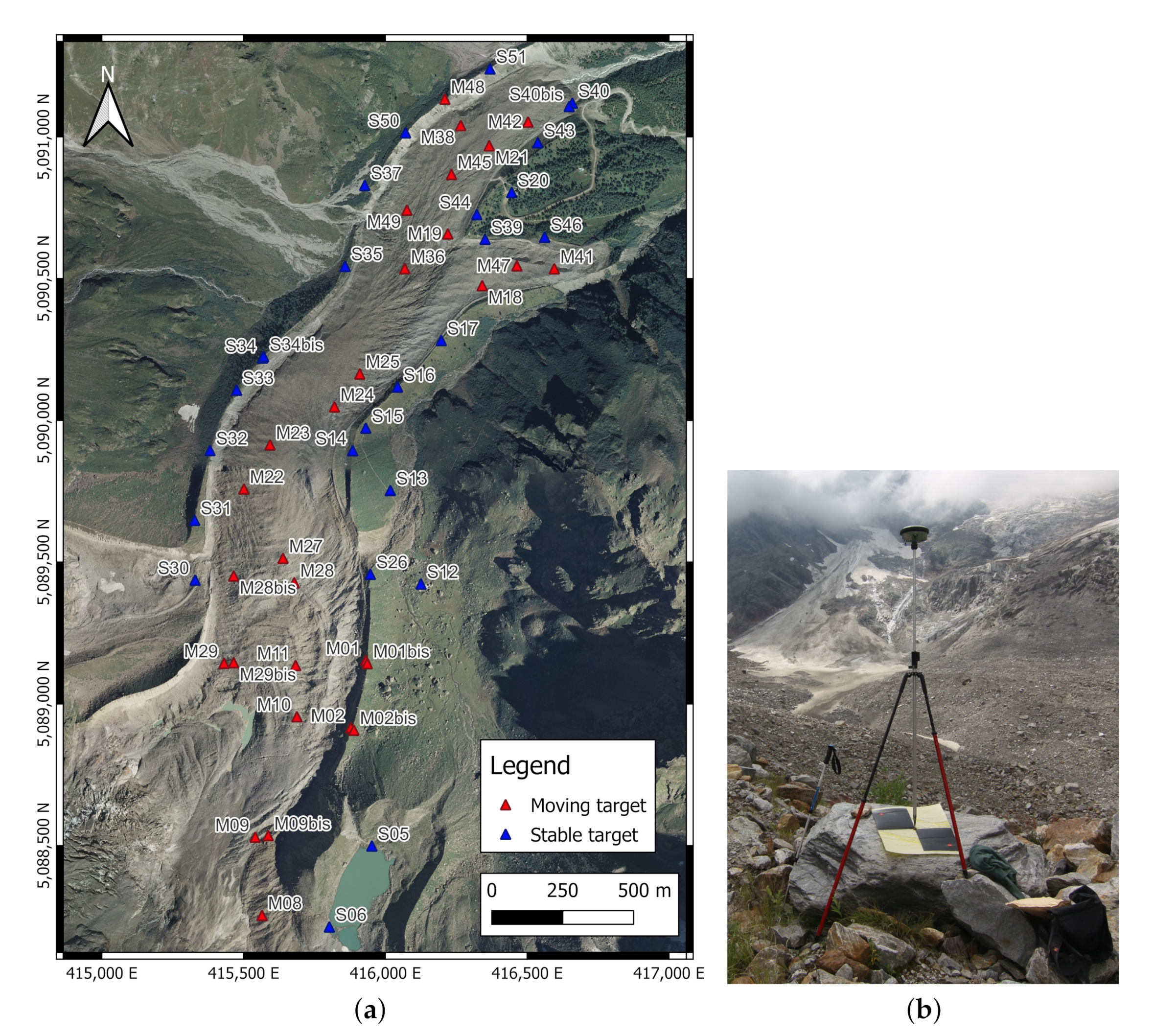
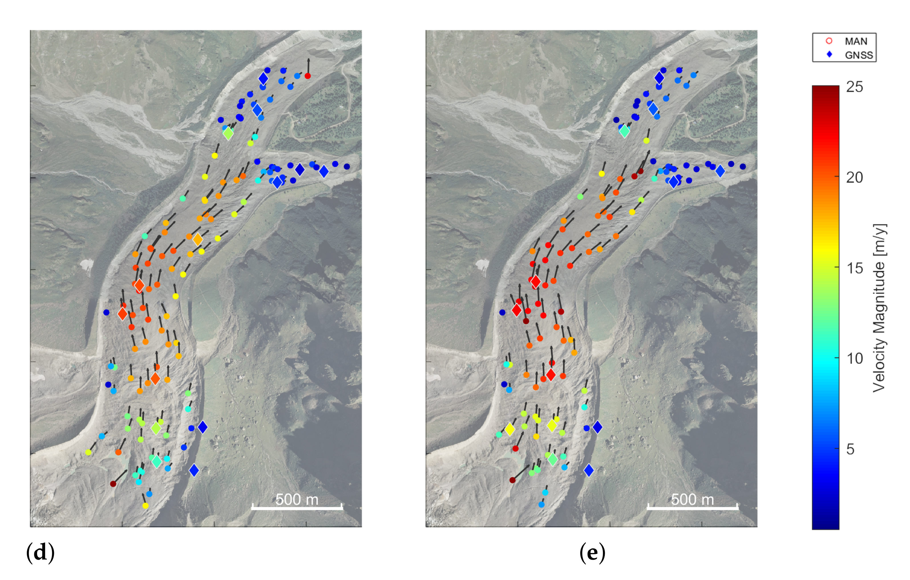
4.1. GNSS Velocity Measurements

Ice flow velocities were first computed from in-situ GNSS measurements of moving targets, deployed over big rocks for photogrammetric purposes (see Section 3.1), Targets coordinates, measured on different years, were differentiated and the annual average velocity of each point was derived by dividing the displacement by the time lag. Figure 5 shows the time-series of the velocities of GNSS points. Most of the moving targets were found and measured for 3 or more years and some of them have been continuously tracked since 2015 (e.g., the point M10 in the upper part of the glacier, M28 in the middle part or M41 on the south-east tongue). However, some of them have been lost over the year, for example, because they fell into a crevasse, and they were replaced with new ones.

The location accuracy of the GNSS measurement was estimated as $\sim 3$ $\mathrm{c}$$\mathrm{m}$ (see Section 3.1). Assuming measurements of the same GCPs at two consecutive years as independent, the expected standard deviation of the velocity was computed by propagating the variance as $\pm 0.04$ $\mathrm{m}$ $\mathrm{y}$⁻¹ (i.e., two order of magnitude less than the computed annual velocities which ranges between 2 m y⁻¹ and 22 $\mathrm{m}$ $\mathrm{y}$⁻¹). Therefore, GNSS measurement are considered as the reference source of information for flow velocity estimation.

From the graph in Figure 5, GNSS points can be visually grouped into three clusters (C1, C2, C3) on the basis of velocity magnitude. The first low-velocity cluster C1 includes points with velocities between 2 m y⁻¹ and 7 $\mathrm{m}$ $\mathrm{y}$⁻¹. The location of GNSS points included in C1 well match morphological sectors S1 (upper accumulation sector) and S3 (glacier tongues), marked in Figure 1a. By contrast, cluster C3 presents significantly higher speed, ranging between 17 m y⁻¹ and 22 $\mathrm{m}$ $\mathrm{y}$⁻¹ were sensed in the central sector S2 (e.g., M10, M11, M22, M28). Cluster C2 include GNSS points located in transition areas between S2 and S1 (e.g., targets M10, M11, placed between the central sector and the accumulation area) and between S2 and S3 (e.g., M49, between the central sector and the lower north-west tongue).

Measurements of targets M22, M23 and M28 suggests the presence of a rising velocity trend in the central part of the glacier between 2018 and 2020. In fact, these points experienced an increase of the velocity magnitude of $\sim 1$ $\mathrm{m}$ $\mathrm{y}$⁻¹ from 2018 to 2020. However, some more measurement years would be necessary to state if this increasing velocity trend holds and is significant. On the other hand, all the other targets showed rather steady velocities over the 6 years.

4.2. MAN Velocity Measurements

The number of GNSS measurements are limited to a dozen of points spread over the glacier, consequently they are not enough to derive a complete glacier velocity field. Hence, other techniques were explored: algorithms, such as normalized cross-correlation [11] or ensemble matching [12], are widely applied to automatically compute displacement on orthophotos and might allow for sub-pixel accuracy [50]. However, because of the presence of snow and due to significantly different environmental conditions between years (Figure 4), it was not feasible to apply automatic image matching algorithms on all the orthophotos to obtain displacements between corresponding pattern of pixels. Therefore, the visual collimation of characteristic features (e.g., sharp edges of big rocks emerging from the snow) on different orthophotos was the only possibility to track elements on the glacier surface. Even though manual collimation precision of natural elements, such as rocks, on orthophotos was likely worse compared to computer vision algorithms, a human operator supervision ensured high matching reliability. Moreover, it was possible to define a regular grid of 100 m × 100 m on the orthophotos in order to select homogeneously distributed features ( $\sim 1$ $\mathrm{pt}$ every 10,000 m${}^2$), resulting in a total of $\sim 130$ points. Most of the points were tracked over the years; however some were lost and only 115 points were found on the 2020 orthophoto.

Assuming collimation standard deviation of $\sim 2$ $\mathrm{px}$ and considering the planimetric accuracy of the orthophotos of $\sim 0.1$ $\mathrm{m}$ (Figure 3), the standard deviation of the velocity obtained from MAN points was estimated as $\pm 0.3$ m/y by variance propagation (covariances were neglected, assuming the orthophotos as independent).

East and North components of all the velocity vectors (i.e., GNSS and MAN computed from all the epochs) are plotted one versus the other in Figure 6. Two main clusters of velocities were identify by k-means clustering and two bivariate Gaussian distribution were fitted to the empirical data [51]. The first cluster, characterized by low velocities, corresponds to C1, identified for GNSS points only in Figure 5. This cluster identifies points located in the accumulation sector or at the glacier tongues. The second cluster consists of higher velocity vectors and corresponds to cluster C3. The points located in between the two main cluster corresponds to transitions areas.

MAN points with (at least) one component that differ more than 2.5 times the standard deviation of each Gaussian model were considered as outliers and rejected. Only 5% of the MAN points were removed (29 out of 609 vectors), highlighting that the velocity measurements obtained by manual collimation on orthophotos match well with the more accurate GNSS measurements.

In Figure 6, four GNSS measurements (labelled with the corresponding target name) and four MAN measurements show a rather strong negative East velocity component, compared to the other points of the low-velocity cluster. These points are located along the right glacier moraine (Figure 6b), which is sliding down towards the glacier body, and therefore rocks on the moraine are moving towards the West (explaining the negative vE component). These points along the moraine have a different dynamics compared to the glacier flow, and consequently they were excluded from the estimation of the main glacier flow velocity field. Finally, the velocity measured on point M22 during the year 2019–2020 presents a strong negative component in the east direction. This might be due to local glacier dynamics, such as the formation of crevasses, which caused the rock to roll or fall with different dynamics than the glacier flow.

For each year, punctual velocity information derived from GNSS and MAN measurements is plotted together in Figure 7. Between 2018 and 2020 (Figure 7e), slightly higher velocities than those of previous years were found in the central part of the glacier, in agreement with the more accurate GNSS measurements presented in Figure 5. However, additional measurement years are necessary in order to statistically prove the existence of an accelerated ice flow of the central sector of the Belvedere Glacier.

4.3. Average Surface Velocity of the Belvedere Glacier during the Period 2015–2020

After having removed the outliers, MAN and GNSS velocity vectors from each year were interpolated over a regular grid with step of 50 m × 50 m, by using a natural neighbour interpolation algorithm [52]. The interpolation grid was kept fixed for all the years in such a way as to arrange the sequence of surface velocity fields into a 3D matrix in which the third dimension is the temporal one.

For each cell of the grid, mean and the standard deviation of the time series of the interpolated velocity vectors were computed, and the results are shown in Figure 8. The map of the standard deviation of the velocity vectors (Figure 8b) highlights that the largest standard deviation (between 1.5 m y⁻¹ and 2 $\mathrm{m}$ $\mathrm{y}$⁻¹) is located in strongly crevassed areas, such as the region above the tongue division or near the sharp bend in the middle of the glacier, and in the accumulation zone. In these regions, thus, there is the largest velocity variability among the years. Elsewhere, the standard deviation is smaller than $1.5$ $\mathrm{m}$ $\mathrm{y}$⁻¹.

5. Ice Volume Variations

To compute glacier volume variation $\Delta V$, consecutive DSMs were differentiated by employing a DEM of Difference (DOD) approach with the tool Compute 2.5D volume implemented in CloudCompare [53]. First, photogrammetric dense clouds were gridded by projecting points along the vertical direction on a planar surface, obtaining DSMs with a cell footprint on ground of 0.5 m × 0.5 m. The choice of the raster resolution was a compromise to achieve a robust height field estimation by averaging a large enough number of points for each cell of the raster, but at the same time small enough to maintain a spatial resolution able to map small scale glacier morphology. A mask was manually created and applied to all the DSMs to exclude areas outside the glacier surface. DSMs from consecutive years were then differentiated pixel-by-pixel to obtain the height difference at each cell of the raster. The volume variation is then computed as:

$$\Delta V^{(i+1,i)}=A_c\times \left({\mathit{e}}^t[{\mathit{z}}^{(i+1)}-{\mathit{z}}^{\left(i\right)}]\right)\left[{\mathrm{m}}^3\right],$$

(1)

where $\mathit{e}$ is a unitary vector with length equal to the number of cells of the DSM, ${\mathit{z}}^{(i+1)}$ and ${\mathit{z}}^{\left(i\right)}$ are respectively vectors containing the height of cells in the DSMs at the year ${}^{(i+1)}$ and at the year ${}^{\left(i\right)}$; $A_c$ is the area of each cell.

In order to rigorously estimate volume variation variances, by propagating the variance, it would be necessary to know the covariance matrix of each DSM, considered as a multivariate random variable with dimension equal to the number of cells. However, no information concerning cells covariances was provided by the SfM software employed, thus it was troublesome to compute covariances between nearby cells in a DSM (which are clearly correlated because they were generated by the same set of images in the photogrammetric process). As a consequence, only a rough estimation of the variance was carried out by considering each DSM as a mono-dimensional random variable with variance equal to the squared value of the vertical component of RMSE computed on the CPs of the relative photogrammetric model (see Figure 3). Moreover, $DS{M}^{(i+1)}$ and $DS{M}^{\left(i\right)}$ were considered as independent because there was no relation between the surveys. The variance of the volume variation was therefore computed as:

$${\sigma }_{\Delta V^{(i+1,i)}}^2={(n\times A_c)}^2\left({\sigma }_{DS{M}^{(i+1)}}^2+{\sigma }_{DS{M}^{\left(i\right)}}^2\right),$$

(2)

where n is the number of cell in the DSMs.

For the years 2015–2016, 2016–2017, 2017–2018, the glacier was partially covered by snow (see Figure 4a–c), which introduced additional uncertainties in volume estimation. The snow height accumulated at the nivometric station located near Zamboni Zappa Hut (2075 m a.s.l., in the central sector of the glacier) on the survey dates was retrieved from the meteorogical database of ARPA Piemonte, the regional agency for the environment [54]: 22 $\mathrm{c}$$\mathrm{m}$ of snow were measured on 23 October 2015, 20 $\mathrm{c}$$\mathrm{m}$ on 20 October 2016, 40 $\mathrm{c}$$\mathrm{m}$ on 15 November 2017. The measured snow heights were considered as additional components of DSM standard deviations. Yet, because the glacier was only partially covered by snow, the snow-driven uncertainty was weighted by half of the total glacier area in variance propagation. Figure 9 illustrates the loss of ice volume year by year. The estimated variance of the glacier volume variation is plotted as an error bar for each value of volume variation.

Between 2017 and 2018, fieldworks were moved from Autumn to Summer. Therefore, the loss of volume for the year 2017–2018 was computed between October 2017 and July 2018, therefore it represented only the variation occurred in wintertime and springtime, and it should not be directly compared with the annual average. Indeed, 2017–2018 volume variation was $-0.75 \times {10}^6$ ${\mathrm{m}}^3$, against the average variation between 2015 and 2020 of $-2.81 \times {10}^6$ ${\mathrm{m}}^3$ (difference of 27%). Ice volume loss for the year 2019–2020 may be slightly underestimated as well: the photogrammetric model of the upper part of the glacier was affected by a larger geometric (RMSE in vertical direction of $=0.28$ $\mathrm{m}$, see Section 3.3) compared to the others models, due to the lack of GCPs measured in-situ at the time of the photo acquisition. Overall, the negative ice volume variation occurred between 2015 and 2020 is evident and significant: every year, between 2 × 10⁶ m³ and 3.5 × 10⁶ ${\mathrm{m}}^3$ of ice were lost.

In Figure 10, elevation profiles of the glacier obtained every year at four different cross sections are plotted together. In each profile, it is easily identifiable the glacier surface, which is delimited by the lateral moraines. The highest height reduction is found at the lower terminus of the glacier (Figure 10a,b): $\sim 2$ $\mathrm{m}$ have been lost every year. It is noticeable that the overall glacier surface profile remained the same, but the ice thickness shrank. In the central part of the glacier (sections CC’ and DD’, Figure 10c,d), the height reduction was less regular because of the crevasses that strongly ripple the transfer zone of the glacier.

6. Comparison with Previous Studies

Several studies focused on understanding and quantifying Belvedere Glacier dynamics. Reference [10] estimated velocities ranging between 32 m y⁻¹ and 43$\mathrm{m}$ $\mathrm{y}$⁻¹ on the whole Belvedere Glacier from October 1995 to September 1999, by employing aerial images. Besides, velocities between 100 m y⁻¹ and 200 $\mathrm{m}$ $\mathrm{y}$⁻¹ were estimated by [10] in Autumn 2001, during the extraordinary surge event of 2000–2001. Nowadays, the Belvedere Glacier is clearly moving slower compared to the late 1990s. However, to the best of authors knowledge, there are no recent works estimating glacier flow velocities.

Concerning volume variations, Reference [37] digitalized two large-scale topographic maps to interpolate DSMs and estimate volume variations between 1957 and 1991. They found a positive volume difference of $+22.7 \times {10}^6$ ${\mathrm{m}}^3$ (with an average rate of $\sim 0.69 \times {10}^6$ ${\mathrm{m}}^3$ ${\mathrm{y}}^{-1}$, roughly assuming a linear volume variation during the years). Their result matched with the study of [6], who estimated an increase of the glacier height of $+1.5$ $\mathrm{m}$ ${\mathrm{y}}^{-1}$ between 1983 and 1985. Recently, ref. [43] used historical aerial images and UAVs to photogrammetrically reconstruct glacier volume variations between 1977 and 2019. For the period 1977–1991, they confirmed the glacier expansion, with a volume increase of $+10.06 \times {10}^6$ ${\mathrm{m}}^3$ ($+0.72 \times {10}^6$ ${\mathrm{m}}^3$ ${\mathrm{y}}^{-1}$). The expansion continued up to 2001 (at the end of the surge event), with additional $10.61 \times {10}^6$ ${\mathrm{m}}^3$ of ice gained. Since 2001, a severe glacier retreat has begun, with a loss of ice volume of $-47.78 \times {10}^6$ ${\mathrm{m}}^3$ ($-5.97 \times {10}^6$ ${\mathrm{m}}^3$ ${\mathrm{y}}^{-1}$) between 2001 and 2009. For the time-span 2009–2019, ref. [43] derived a negative variation of $-27.16 \times {10}^6$ ${\mathrm{m}}^3$ of ice ($-2.72 \times {10}^6$ ${\mathrm{m}}^3$ ${\mathrm{y}}^{-1}$). This last ten-years-averaged estimate well matches with the annual volume variations found in this study between 2015 and 2020 (between −2 × 10⁶ m³ y⁻¹ and −3.5 × 10⁶ ${\mathrm{m}}^3$ ${\mathrm{y}}^{-1}$).

7. Conclusions

This work presents the results of a mid-term monitoring campaign carried out with low-cost UAVs on the debris-covered Belvedere Glacier between 2015 and 2020, to quantify ice flow velocities and volume variations. During yearly fieldworks, several flights with fixed-wing UAVs and quadcopters were executed to acquire images with GSD ranging between 5 cm and 9 $\mathrm{c}$$\mathrm{m}$. Moreover, a set of GCPs and CPs was deployed, checked and measured every year with topographic-grade GNSS receivers. These were used respectively for image orientation and for photogrammetric blocks validation. Acquired data were processed by means of SfM-MVS techniques to obtain decimetric-accurate 3D models, orthophotos and DSMs. Annual glacier velocity was derived by in-situ GNSS measurements of photogrammetric targets, combined with more dense features, manually collimated on orthophotos. To this end, ∼12 equally-spaced natural features, such as rock edges, were tracked over the years. The accuracy of the GNSS-derived velocity vectors was estimated as $\pm 0.04$ $\mathrm{m}$ ${\mathrm{y}}^{-1}$, whereas the accuracy of the orthophoto-based velocities was $\pm 0.3$ $\mathrm{m}$ ${\mathrm{y}}^{-1}$. A good agreement between the two approaches was found, and complete annual velocity fields were derived by combining them. Velocities ranging between 17 m y⁻¹ and 22 $\mathrm{m}$ ${\mathrm{y}}^{-1}$ were found in the central part of the glacier, whereas values between 2 m y⁻¹ and 7 $\mathrm{m}$ ${\mathrm{y}}^{-1}$ were found in the accumulation area and at the glacier terminus. To estimate annual ice volume variations, photogrammetric DSMs with cell size of 0.5 m × 0.5 m were differentiated pixel-by-pixel. Between 2 × 10⁶ m³ and 3.5 × 10⁶ ${\mathrm{m}}^3$ of ice were lost every year. Volume variation accuracy was estimated on the basis of photogrammetric models RMSE in the vezrtical direction, resulting in uncertainties ranging between 0.2 × 10⁶ m³ and 0.4 × 10⁶ ${\mathrm{m}}^3$. One pair of intra-year measurements (October 2017–July 2018) highlighted that the ice volume variation occurred during winter and spring 2017–2018 was ∼1/4 of the average annual ice loss computed from 2015 to 2020 ($0.75 \times {10}^6$ ${\mathrm{m}}^3$ against $2.81 \times {10}^6$ ${\mathrm{m}}^3$).

Our 6-year monitoring campaign suggests the potentials of UAVs for periodical cryosphere monitoring, in particular for small alpine glaciers such as the Belvedere Glacier. High-resolution photogrammetric models, DSMs and orthophotos derived by UAVs may have great value in glaciological studies for understanding the glacier dynamics both in terms of mass changes and kinematics, as well as for validating mass balance models of glaciers [55,56]. The variation of glacier volume can be used in two different issues of hydrologic balance: (1) as control on the ice melting volume, in a similar manner to the one proposed by [57], where the snow volume accumulated at the end of accumulation season has been used as control for the volume of the melting snow; or (2) separating the different melt water sources (ice from snow) in river flow [58]. These issues are of a certain importance in hydrological modelling, because in the absence of control on the melting water of ice, the hydrological model (which generally treats the glacier as constant) may overestimate the melting, also generating an overestimation of the water discharge, as clearly shown in [57]. Similarly, distinguishing the different melting water contributions is important to investigate the impacts of climate changes on the different water compartments and consequently, the impacts on the connected water uses, as, for example, the hydropower production [59,60].

Overall, our study highlights that decimetric-accurate photogrammetric models can be periodically obtained by using low-cost UAVs and cameras. This high geometrical resolution and accuracy is not yet achievable by employing satellite imageries or aerial platforms, and it may be relevant for hydrological analysis, for example, mass balances. Indeed, uncertainties in photogrammetric models translate in errors in volume ice volume variation and, consequently, melting water of ice estimation. Moreover, UAVs require minimal data acquisition costs and allow for great surveying flexibility. In fact, despite the harsh environment, in-situ operations were limited to a few days to successfully gather information on the whole glacier. Therefore, UAVs can be employed by small research groups or environmental agencies to carry out yearly or seasonal monitoring activities.

References

1. Oerlemans, J. Extracting a Climate Signal from 169 Glacier Records. Science 2005, 308, 675–677. [Google Scholar] [CrossRef] [PubMed] [Green Version]
2. Barry, R.G. The status of research on glaciers and global glacier recession: A review. Prog. Phys. Geog. Earth Environ. 2016, 30, 285–306. [Google Scholar] [CrossRef]
3. Zemp, M.; Haeberli, W.; Hoelzle, M.; Paul, F. Alpine glaciers to disappear within decades? Geophys. Res. Lett. 2006, 33. [Google Scholar] [CrossRef] [Green Version]
4. Sommer, C.; Malz, P.; Seehaus, T.C.; Lippl, S.; Zemp, M.; Braun, M.H. Rapid glacier retreat and downwasting throughout the European Alps in the early 21st century. Nat. Commun. 2020, 11, 3209. [Google Scholar] [CrossRef] [PubMed]
5. Zekollari, H.; Huss, M.; Farinotti, D. Modelling the future evolution of glaciers in the European Alps under the EURO-CORDEX RCM ensemble. Cryosphere 2019, 13, 1125–1146. [Google Scholar] [CrossRef] [Green Version]
6. Roethlisberger, H.; Haeberli, W.; Schmid, W.; Biolzi, M.; Pika, J. Studi Sul Comportamento Del Ghiacciao Del Belvedere; Report 97.3; Comunità montana della Valle Anzasca: Macugnaga, VB, Italy, 1985. [Google Scholar] [CrossRef]
7. Kääb, A.; Funk, M. Modelling mass balance using photogrammetric and geophysical data: A pilot study at Griesgletscher, Swiss Alps. J. Glaciol. 1999, 45, 575–583. [Google Scholar] [CrossRef] [Green Version]
8. Eder, K.; Würländer, R.; Rentsch, H. Digital photogrammetry for the new Glacier Inventory Of Austria. Int. Arch. Photogramm. Remote Sens. 2000, XXXIII, 254–261. [Google Scholar]
9. Scambos, T.A.; Dutkiewicz, M.J.; Wilson, J.C.; Bindschadler, R.A. Application of image cross-correlation to the measurement of glacier velocity using satellite image data. Remote Sens. Environ. 1992, 42, 177–186. [Google Scholar] [CrossRef]
10. Kääb, A.; Huggel, C.; Fischer, L.; Guex, S.; Paul, F.; Roer, I.; Salzmann, N.; Schlaefli, S.; Schmutz, K.; Schneider, D.; et al. Remote sensing of glacier-and permafrost-related hazards in high mountains: An overview. Nat. Hazard Earth Sys. 2005, 5, 527–554. [Google Scholar] [CrossRef]
11. Heid, T.; Kääb, A. Evaluation of existing image matching methods for deriving glacier surface displacements globally from optical satellite imagery. Remote Sens. Environ. 2012, 118, 339–355. [Google Scholar] [CrossRef]
12. Altena, B.; Kääb, A. Ensemble matching of repeat satellite images applied to measure fast-changing ice flow, verified with mountain climber trajectories on Khumbu icefall, Mount Everest. J. Glaciol. 2020, 66, 905–915. [Google Scholar] [CrossRef]
13. Zhou, Y.; Chen, J.; Cheng, X. Glacier Velocity Changes in the Himalayas in Relation to Ice Mass Balance. Remote Sens. 2021, 13, 3825. [Google Scholar] [CrossRef]
14. Strozzi, T.; Kouraev, A.; Wiesmann, A.; Wegmüller, U.; Sharov, A.; Werner, C. Estimation of Arctic glacier motion with satellite L-band SAR data. Remote Sens. Environ. 2008, 112, 636–645. [Google Scholar] [CrossRef]
15. Fang, L.; Xu, Y.; Yao, W.; Stilla, U. Estimation of glacier surface motion by robust phase correlation and point like features of SAR intensity images. ISPRS J. Photogramm. Remote Sens. 2016, 121, 92–112. [Google Scholar] [CrossRef]
16. Strozzi, T.; Caduff, R.; Jones, N.; Barboux, C.; Delaloye, R.; Bodin, X.; Kääb, A.; Mätzler, E.; Schrott, L. Monitoring Rock Glacier Kinematics with Satellite Synthetic Aperture Radar. Remote Sens. 2020, 12, 559. [Google Scholar] [CrossRef] [Green Version]
17. Fieber, K.D.; Mills, J.P.; Miller, P.E.; Clarke, L.; Ireland, L.; Fox, A.J. Rigorous 3D change determination in Antarctic Peninsula glaciers from stereo WorldView-2 and archival aerial imagery. Remote Sens. Environ. 2018, 205, 18–31. [Google Scholar] [CrossRef]
18. Giulio Tonolo, F.; Cina, A.; Manzino, A.; Fronteddu, M. 3D glacier mapping by means of satellite stereo images: The Belvedere Glacier case study in the Italian Alps. Int. Arch. Photogramm. Remote Sens. Spatial Inf. Sci. 2020, 43, 1073–1079. [Google Scholar] [CrossRef]
19. Westoby, M.; Brasington, J.; Glasser, N.; Hambrey, M.; Reynolds, J. ‘Structure-from-Motion’ photogrammetry: A low-cost, effective tool for geoscience applications. Geomorphology 2012, 179, 300–314. [Google Scholar] [CrossRef] [Green Version]
20. Seitz, S.M.; Curless, B.; Diebel, J.; Scharstein, D.; Szeliski, R. A comparison and evaluation of multi-view stereo reconstruction algorithms. In Proceedings of the IEEE Computer Society Conference on Computer Vision and Pattern Recognition, New York, NY, USA, 17–22 June 2006; Volume 1, pp. 519–526. [Google Scholar] [CrossRef]
21. Cook, K.L. An evaluation of the effectiveness of low-cost UAVs and structure from motion for geomorphic change detection. Geomorphology 2017, 278, 195–208. [Google Scholar] [CrossRef]
22. James, M.R.; Robson, S.; Smith, M.W. 3-D uncertainty-based topographic change detection with structure-from-motion photogrammetry: Precision maps for ground control and directly georeferenced surveys. Earth Surf. Proc. Land. 2017, 42, 1769–1788. [Google Scholar] [CrossRef]
23. Detert, M.; Johnson, E.D.; Weitbrecht, V. Proof-of-concept for low-cost and non-contact synoptic airborne river flow measurements. Int. J. Remote Sens. 2017, 38, 2780–2807. [Google Scholar] [CrossRef]
24. Ioli, F.; Pinto, L.; Passoni, D.; Nova, V.; Detert, M. Evaluation of Airborne Image Velocimetry Approaches Using Low-Cost UAVs in Riverine Environments. Int. Arch. Photogramm. Remote Sens. Spatial Inf. Sci. 2020, 43, 597–604. [Google Scholar] [CrossRef]
25. De Michele, C.; Avanzi, F.; Passoni, D.; Barzaghi, R.; Pinto, L.; Dosso, P.; Ghezzi, A.; Gianatti, R.; Vedova, G.D. Using a fixed-wing UAS to map snow depth distribution: An evaluation at peak accumulation. Cryosphere 2016, 10, 511–522. [Google Scholar] [CrossRef] [Green Version]
26. Buhler, Y.; Adams, M.S.; Bosch, R.; Stoffel, A. Mapping snow depth in alpine terrain with unmanned aerial systems (UASs): Potential and limitations. Cryosphere 2016, 10, 1075–1088. [Google Scholar] [CrossRef] [Green Version]
27. Avanzi, F.; Bianchi, A.; Cina, A.; De Michele, C.; Maschio, P.; Pagliari, D.; Passoni, D.; Pinto, L.; Piras, M.; Rossi, L. Centimetric accuracy in snow depth using unmanned aerial system photogrammetry and a multistation. Remote Sens. 2018, 10, 765. [Google Scholar] [CrossRef] [Green Version]
28. Pagliari, D.; Rossi, L.; Passoni, D.; Pinto, L.; Michele, C.D.; Avanzi, F. Measuring the volume of flushed sediments in a reservoir using multi-temporal images acquired with UAS. Geomat. Nat. Haz. Risk 2016, 8, 150–166. [Google Scholar] [CrossRef]
29. Bhardwaj, A.; Sam, L.; Akanksha; Martín-Torres, F.J.; Kumar, R. UAVs as remote sensing platform in glaciology: Present applications and future prospects. Remote Sens. Environ. 2016, 175, 196–204. [Google Scholar] [CrossRef]
30. Whitehead, K.; Moorman, B.J.; Hugenholtz, C.H. Brief Communication: Low-cost, on-demand aerial photogrammetry for glaciological measurement. Cryosphere 2013, 7, 1879–1884. [Google Scholar] [CrossRef] [Green Version]
31. Immerzeel, W.W.; Kraaijenbrink, P.D.; Shea, J.M.; Shrestha, A.B.; Pellicciotti, F.; Bierkens, M.F.; de Jong, S.M. High-resolution monitoring of Himalayan glacier dynamics using unmanned aerial vehicles. Remote Sens. Environ. 2014, 150, 93–103. [Google Scholar] [CrossRef]
32. Kraaijenbrink, P.; Meijer, S.W.; Shea, J.M.; Pellicciotti, F.; de Jong, S.M.; Immerzeel, W.W. Seasonal surface velocities of a Himalayan glacier derived by automated correlation of unmanned aerial vehicle imagery. Ann. Glaciol. 2016, 57, 103–113. [Google Scholar] [CrossRef] [Green Version]
33. Gindraux, S.; Boesch, R.; Farinotti, D. Accuracy Assessment of Digital Surface Models from Unmanned Aerial Vehicles’ Imagery on Glaciers. Remote Sens. 2017, 9, 186. [Google Scholar] [CrossRef] [Green Version]
34. Jouvet, G.; van Dongen, E.; Lüthi, M.P.; Vieli, A. In situ measurements of the ice flow motion at Eqip Sermia Glacier using a remotely controlled unmanned aerial vehicle (UAV). Geosci. Instrum. Meth. 2020, 9, 1–10. [Google Scholar] [CrossRef] [Green Version]
35. Cao, B.; Guan, W.; Li, K.; Pan, B.; Sun, X. High-Resolution Monitoring of Glacier Mass Balance and Dynamics with Unmanned Aerial Vehicles on the Ningchan No. 1 Glacier in the Qilian Mountains, China. Remote Sens. 2021, 13, 2735. [Google Scholar] [CrossRef]
36. Benoit, L.; Gourdon, A.; Vallat, R.; Irarrazaval, I.; Gravey, M.; Lehmann, B.; Prasicek, G.; Gräff, D.; Herman, F.; Mariethoz, G. A high-resolution image time series of the Gorner Glacier – Swiss Alps – derived from repeated unmanned aerial vehicle surveys. Earth Syst. Sci. Data 2019, 11, 579–588. [Google Scholar] [CrossRef] [Green Version]
37. Diolaiuti, G.; D’Agata, C.; Smiraglia, C. Belvedere Glacier, Monte Rosa, Italian Alps: Tongue Thickness and Volume Variations in the Second Half of the 20th Century. Arct. Antarct. Alp. Res. 2003, 35, 255–263. [Google Scholar] [CrossRef]
38. Haeberli, W.; Kääb, A.; Paul, F.; Chiarle, M.; Mortara, G.; Mazza, A.; Deline, P.; Richardson, S. A surge-type movement at Ghiacciaio del Belvedere and a developing slope instability in the east face of Monte Rosa, Macugnaga, Italian Alps. Nor. Geogr. Tidsskr. 2002, 56, 104–111. [Google Scholar] [CrossRef]
39. Monterin, U. Il Ghiacciaio di Macugnaga dal 1870 al 1922. Bolletino Com. Glaciol. Ital. 1923, 5, 12–40. [Google Scholar]
40. Mazza, A. Evolution and dynamics of Ghiacciaio Nord delle Locce (Valle Anzasca, Western Alps) from 1854 to the present. Geogr. Fis. Din. Quat. 1998, 21, 233–243. [Google Scholar]
41. Kääb, A.; Huggel, C.; Barbero, S.; Chiarle, M.; Cordola, M.; Epifani, F.; Haeberli, W. Glacier Hazards At Belvedere Glacier and the Monte Rosa East Face, Italian Alps: Processes and Mitigation. Int. Symp. Interpraevent–Riva/Trient 2004, 1, 67–78. [Google Scholar]
42. Noferini, L.; Mecatti, D.; Macaluso, G.; Pieraccini, M.; Atzeni, C. Monitoring of Belvedere Glacier using a wide angle GB-SAR interferometer. J. Appl. Geophys. 2009, 68, 289–293. [Google Scholar] [CrossRef]
43. De Gaetani, C.I.; Ioli, F.; Pinto, L. Aerial and UAV Images for Photogrammetric Analysis of Belvedere Glacier Evolution in the Period 1977–2019. Remote Sens. 2021, 13, 3787. [Google Scholar] [CrossRef]
44. Mölg, N.; Ferguson, J.; Bolch, T.; Vieli, A. On the influence of debris cover on glacier morphology: How high-relief structures evolve from smooth surfaces. Geomorphology 2020, 357, 107092. [Google Scholar] [CrossRef]
45. Mortara, G.; Tamburini, A.; Ercole, G.; Semino, P.; Chiarle, M.; Godone, F.; Guiliano, M.; Haeberli, W.; Kääb, A.; Huggel, C.; et al. Il Ghiacciaio del Belvedere e L’emergenza del Lago Effimero; Regione Piemonte; Societa’ Meteorologica Subalpina: Moncalieri, TO, Italy, 2009. [Google Scholar]
46. Agisoft Metashape. Available online: https://www.agisoft.com (accessed on 25 October 2021).
47. Fraser, C.S. Automatic camera calibration in close range photogrammetry. Photogramm. Eng. Remote. Sens. 2013, 79, 381–388. [Google Scholar] [CrossRef] [Green Version]
48. Cramer, M.; Przybilla, H.J.; Zurhorst, A. UAV cameras: Overview and geometric calibration benchmark. Int. Arch. Photogramm. Remote Sens. Spat. Inf. Sci. 2017, 42, 85–92. [Google Scholar] [CrossRef] [Green Version]
49. Dall’asta, E.; Roncella, R. A comparison of semiglobal and local dense matching algorithms for surface reconstruction. Int. Arch. Photogramm. Remote Sens. Spatial Inf. Sci. 2014, XL-5, 187–194. [Google Scholar] [CrossRef] [Green Version]
50. Debella-Gilo, M.; Kääb, A. Sub-pixel precision image matching for measuring surface displacements on mass movements using normalized cross-correlation. Remote Sens. Environ. 2011, 115, 130–142. [Google Scholar] [CrossRef] [Green Version]
51. McLachlan, G.; Peel, D. Finite Mixture Models; John Wiley & Sons: New York, NY, USA, 2000. [Google Scholar]
52. Sibson, R. A Brief Description of Natural Neighbor Interpolation; John Wiley & Sons: New York, NY, USA, 1981; pp. 21–36. [Google Scholar]
53. CloudCompare. Available online: https://www.cloudcompare.org (accessed on 25 October 2021).
54. Arpa Piemonte. Available online: https://www.arpa.piemonte.it/rischinaturali/accesso-ai-dati/annali_meteoidrologici/annali-meteo-idro/banca-dati-meteorologica.html (accessed on 25 October 2021).
55. Gerbaux, M.; Genthon, C.; Etchevers, P.; Vincent, C.; Dedieu, J. Surface mass balance of glaciers in the French Alps: Distributed modeling and sensitivity to climate change. J. Glaciol. 2005, 51, 561–572. [Google Scholar] [CrossRef] [Green Version]
56. Machguth, H.; Paul, F.; Hoelzle, M.; Haeberli, W. Distributed glacier mass-balance modelling as an important component of modern multi-level glacier monitoring. Ann. Glaciol. 2006, 43, 335–343. [Google Scholar] [CrossRef] [Green Version]
57. Bavera, D.; De Michele, C.; Pepe, M.; Rampini, A. Melted snow volume control in the snowmelt runoff model using a snow water equivalent statistically based model. Hydrol. Process. 2012, 26, 3405–3415. [Google Scholar] [CrossRef]
58. Armstrong, R.; Rittger, K.; Brodzik, M.; Racoviteanu, A.; Barrett, A.; Singh Khalsa, S.; Raup, B.; Hill, A.; Khan, A.; Wilson, A.; et al. Runoff from glacier ice and seasonal snow in High Asia: Separating melt water sources in river flow. Reg. Environ. Chang. 2019, 19, 1249–1261. [Google Scholar] [CrossRef] [Green Version]
59. Gaudard, L.; Avanzi, F.; De Michele, C. Seasonal aspects of the energy-water nexus: The case of a run-of-the-river hydropower plant. Appl. Energy 2018, 210, 604–612. [Google Scholar] [CrossRef]
60. Patro, E.; De Michele, C.; Avanzi, F. Future perspectives of run-of-the-river hydropower and the impact of glaciers’ shrinkage: The case of Italian Alps. Appl. Energy 2018, 231, 699–713. [Google Scholar] [CrossRef]
Figure 1. (a) Location of the Belvedere Glacier with superimposed the three main morphological sectors: sector 1 (S1) is the accumulation zone, sector 2 (S2) is the transfer zone, sector 3 (S3) is the low-relief zone with the two glacier tongues. Coordinates are framed in ETRF2000(2008)—UTM 32N. [Basemap source: Swisstopo (geo.admin.ch) ]; (b) Photo of the Belvedere Glacier taken by the authors during the 2020 survey.
Remotesensing 14 00028 g001
Figure 2. (a) Location of the targets used for the photogrammetric surveys. For each year, a subset of the targets was used as GCPs, while the remaining as CPs; (b) lan example of a photogrammetric target deployed over the glacier moraine.
Remotesensing 14 00028 g002
Figure 3. Barplot of reprojection RMSE computed CPs for each photogrammetric model. Due to practical problems occurred in 2020 and explained in Section 3.3, the RMSE of 2020 model was split in two parts: 2020 lower denotes the CP RMSE over related to the central and lower sectors of the glacier (S2 and S3 in Figure 1a), whereas 2020 upper refers to the upper accumulation sector only (S1).
Remotesensing 14 00028 g003
Figure 4. Orthophotos obtained from the photogrammetric model for each year: (a) 2015, (b) 2016, (c) 2017, (d) 2018, (e) 2019, (f) 2020.
Remotesensing 14 00028 g004
Figure 5. (a) Time series of the velocity computed from the GNSS measurements of the targets deployed over the glacier. Dashed lines denote measurement continuity over the years (i.e., if the line is interrupted, the target was lost or not measured during that year). Labels C1–C3 denote the three velocity clusters of GNSS points, whereas labels S1–S3 indicate the three morphological sectors marked in Figure 1a. A correspondence between clusters and sectors can be identified: C1 corresponds to sectors S1 and S2, cluster C3 to sector S2, whereas cluster C2 corresponds to the two transition areas S2–S1 and S2–S3. (b) Location of the targets over the glacier.
Remotesensing 14 00028 g005
Figure 6. (a) Scatter plot of the planimetric components (vE-vN) of GNSS and MAN velocity vectors obtained from all the years; (b) Location of the moving GNSS points.
Remotesensing 14 00028 g006
Figure 7. Measured GNSS and MAN velocities for each year: (a) 2015–2016, (b) 2016–2017, (c) 2017–2018, (d) 2018–2019, (e) 2019–2020. Dots represent MAN measurements, diamonds refer to GNSS measurements. Note that the velocity field for 2017–2018 were derived from the surveys of October 2017 and July 2018, and therefore velocities refer mostly to the wintertime and thus they are smaller than the annual ones.
Remotesensing 14 00028 g007aRemotesensing 14 00028 g007b
Figure 8. (a) Mean surface velocity field of the Belvedere Glacier for the period 2015–2020. (b) Standard deviation of the velocity time-series (2015–2020) for each cell of the raster grid. Note that in both (a,b), year 2017–2018 was not considered.
Remotesensing 14 00028 g008
Figure 9. Yearly volume variation computed as difference between DSM of two consecutive years. The error bars plotted represent the uncertainty of each estimated value. Note that the values on the Y axis are expressed in million of m 3 .
Remotesensing 14 00028 g009
Figure 10. Elevation profiles obtained from the DSM computed on the years 2015–2020 along 4 different cross-sections. (a) Cross-section AA’ at the north-west glacier tongue; (b) Cross-section BB’ at the south toungue; (c) Cross-section CC’ in the lower portion of the glacier transition sector; (d) Cross-section DD’ in the upper portion of the glacier transition sector; (e) Cross-sections location. Cross-sections are seen from South towards North (i.e., from upstream to downstream of the glacier), as marked by the letters in (e).
Remotesensing 14 00028 g010