Accounting for Signal Distortion Biases for Wide-Lane and Narrow-Lane Phase Bias Estimation with Inhomogeneous Networks

Abstract

Due to different designs of receiver correlators and front ends, receiver-related pseudorange biases, called signal distortion biases (SDBs), exist. Ignoring SDBs that can reach up to 0.66 cycles and 10 ns in Melbourne-Wübbena (MW) and ionosphere-free (IF) combinations can negatively affect phase bias estimation. In this contribution, we investigate the SDBs and evaluate the impacts on wide-lane (WL) and narrow-lane (NL) phase bias estimations, and further propose an approach to eliminating these SDBs to improve phase bias estimation. Based on a large data set of 302 multi-global navigation satellite system (GNSS) experiment (MGEX) stations, including 5 receiver brands, we analyze the characteristics of these SDBs The SDB characteristics of different receiver types for different GNSS systems differ from each other. Compared to the global positioning system (GPS) and BeiDou navigation satellite system (BDS), SDBs of Galileo are not significant; those of BDS-3 are significantly superior to BDS-2; Septentrio (SEPT) receivers show the most excellent consistency among all receiver types. Then, we apply the corresponding corrections to phase bias estimation for GPS, Galileo and BDS. The experimental results reveal that the calibration can greatly improve the performance of phase bias estimation. For WL phase biases estimation, the consistencies of WL phase biases among different networks for GPS, Galileo, BDS-2 and BDS-3 improve by 89%, 77%, 76% and 78%, respectively. There are scarcely any improvements of the fixing rates for Galileo due to its significantly small SDBs, while for GPS, BDS-2 and BDS-3, the WL ambiguity fixing rates can improve greatly by 13%, 27% and 14% after SDB calibrations with improvements of WL ambiguity fixing rates, the corresponding NL ambiguity fixing rates can further increase greatly, which can reach approximately 16%, 27% and 22%, respectively. Additionally, after the calibration, both WL and NL phase bias series become more stable. The standard deviations (STDs) of WL phase bias series for GPS and BDS can improve by more than 46%, while those of NL phase bias series can yield improvements of more than 13%. Ultimately, the calibration can make more WL and NL ambiguity residuals concentrated in ranges within ±0.02 cycles. All these results demonstrate that SDBs for phase bias estimation cannot be ignored and must be considered when inhomogeneous receivers are used.

1. Introduction

Precise point positioning (PPP) is a high-precision positioning technique that can achieve centimeter-level positioning with a single receiver [1]. However, undifferenced ambiguities cannot be estimated as integers directly, thus limiting the application of PPP [2,3]. In the past decade, several PPP ambiguity resolution (PPP-AR) approaches have been proposed and implemented [2,3,4,5,6]. Ge et al. (2008) [4] utilized satellite phase biases to recover the ambiguity integer property. Laurichesse et al. (2009) [5] and Collins et al. (2008) [6] provided integer or decoupled clock products directly to users by absorbing narrow-lane (NL) phase biases into the satellite clocks. All three methods have been already proven equivalent in theory, but with different expressions [7,8,9].

In PPP-AR, although phase biases are solved to achieve integer ambiguities, but they mainly rely on pseudorange observations. For instance, Melbourne–Wübbena (MW) combination [10,11] is utilized to estimate wide-lane (WL) phase biases, and pseudorange observations are inevitably introduced; in the NL phase bias estimation, precise ionosphere-free (IF) combination ambiguities are obtained first, which also require pseudorange observations. Therefore, phase bias estimation depends heavily on the quality of pseudorange observations.

However, there is a problem of pseudorange biases, called the signal distortion biases (SDBs) due to the different realizations of receiver front-end bandwidth and correlators among different manufacturers [12,13,14,15]. In recent years, more studies are focusing on the SDBs. For instance, Gong et al. (2018) [16] found that for the BeiDou navigation satellite system (BDS)-2, B1/B2 IF pseudorange observations among different types of receivers can reach approximately 3ns, and established correction models of IF combination. Following that, to make these SDBs available for single-frequency users, Zheng et al. (2019) [17] calibrated these biases at each frequency by introducing two additional IF and geometry-free (IFGF) combinations. Additionally, these SDBs greatly influenced satellite differential signal biases (DSBs) and clock estimation. In response to this, Hauschild and Montenbruck (2019) [18] presented a detailed study for different GNSS systems and found that Galileo yielded very consistent DSBs and clock estimation across various receivers, but that for the Global Positioning System (GPS) and BDS-2, the maximum inconsistencies of DSBs and satellite clocks among different receiver networks exceeded 1.0 and 2.5 ns, respectively. Thereafter, the impacts of these SDBs on satellite DSBs and clocks for GPS and Galileo were analyzed systematically, and these biases were calibrated by utilizing the proposed models [19].

It must be pointed out that precise pseudorange measurements are crucial for phase bias estimation and PPP-AR [20,21]. However, the existence of SDBs makes code division multiple access (CDMA) signal similar to frequency division multiple access (FDMA) signal, and these biases cannot be completely absorbed by receiver clocks or phase biases. They can further contaminate the integer feature, thus negatively affecting PPP-AR at the user side. Zheng et al. (2019) [17] proposed a method to eliminate the SDBs to improve the WL ambiguity fixing rate for BDS-2. Furthermore, from the perspective of the WL fractional part of the float ambiguity, Cui et al. (2021) [22] analyzed deviations in WL phase biases and their impacts on the phase bias products and user-side PPP-AR. The deviations in WL phase biases are essentially caused by SDBs.

Although some studies on the characteristics and impacts of SDBs have been done, there are still many aspects out of consideration and investigation. First, there are no BDS-3 SDB corrections available for phase bias estimation. The BDS-3 corrections proposed by Zhang et al. (2021) [23] are mainly applied to dual-frequency IF satellite clock estimation. Second, according to the studies above, the impacts of SDBs on WL phase bias estimation are only a small part of the studies, far from detailed enough. Finally, their impacts on NL phase bias estimation have not been investigated or evaluated so far.

It is clear that ignoring such receiver-related SDBs will negatively affect WL and NL phase bias estimations and even result in error ambiguity fixing for PPP-AR users. In this contribution, we concentrate on the effects of SDBs on WL and NL phase bias estimations and propose a calibration model to improve multi-GNSS satellite phase bias estimation from inhomogeneous stations. Section 2 displays the calibration method of the SDBs in phase bias estimation. In Section 3, based on 302 stations from the Multi-GNSS Experiment (MGEX) network [24], we systematically analyze the characteristics of SDBs for GPS, Galileo, BDS-2 and BDS-3. Furthermore, in Section 4, the calibration is applied to eliminate the impacts on the WL and NL phase bias estimations and evaluate its performance. Finally, Section 5 draws the conclusions.

2. Methods

In this section, we start with the GNSS observational equations and describe the method of phase bias estimation as well as give the calibration model of the receiver-related SDBs.

2.1. Phase Bias Estimation

In GNSS data processing, the raw observations of the GNSS pseudorange and carrier phase are generally expressed as

$$\begin{array}{c}{P}_{r,f}^s={\rho }_r^s+c·t_r-c·t^s+{\alpha }_r^s·T_z+{\beta }_f·I_r^s+c·b_{r,f}-c·b_f^s+{\epsilon }_P\\ L_{r,f}^s={\rho }_r^s+c·t_r-c·t^s+{\alpha }_r^s·T_z-{\beta }_f·I_r^s+{\lambda }_f·\left({\tilde{N}}_{r,f}^s-\phi \right)+{\epsilon }_L\end{array}\}$$

(1)

where $P_{r,f}^s$ and $L_{r,f}^s$ are the raw measurements of the pseudorange and carrier phase from satellite s to receiver r in length units, respectively; $f$ is the carrier frequency of the signal; ${\rho }_r^s$ is the geometric distance, to which antenna phase center corrections and earth rotation correction are applied; $c$ denotes the speed of light in vacuum; $t_r$ and $t^s$ represent the receiver clock offset and satellite clock offset, respectively; $T_z$ is the zenith tropospheric delay, available to be converted to the slant delay through the mapping function ${\alpha }_r^s$; $I_r^s$ represents the line-of-sight total electron content with the frequency-dependent factor ${\beta }_f$; $b_{r,f}$ and $b_f^s$ denote receiver-dependent and satellite-dependent observable-specific signal biases (OSBs), respectively; ${\tilde{N}}_{r,f}^s$ represents the float ambiguity and $\phi$ is the phase wind-up error in the cycle, as well as ${\lambda }_f$ is the corresponding wavelength; ${\epsilon }_P$ and ${\epsilon }_{\mathsf{\Phi }}$ denote the observation noise of the pseudorange and phase.

The MW and IF combination measurements from satellite, s, to receiver, r, are respectively defined as [10]

$${\mathrm{MW}}_r^s=\left(\frac{L_{r,1}^s}{{\lambda }_1}-\frac{L_{r,2}^s}{{\lambda }_2}\right)-\frac{\left(f_1·P_{r,1}^s+f_2·P_{r,2}^s\right)}{\left(f_1+f_2\right)·{\lambda }_{1,-1}}$$

(2)

$$\begin{array}{ll}{P}_{r,\mathrm{IF}}^s& =\frac{f_1^2}{f_1^2-f_2^2}·P_{r,1}^s-\frac{f_2^2}{f_1^2-f_2^2}·P_{r,2}^s\\ & ={\rho }_r^s+c·t_r-c·t^s+{\alpha }_r^s·T_z+c·b_{r,\mathrm{IF}}-c·b_{\mathrm{IF}}^s+{\epsilon }_{P,\mathrm{IF}}\end{array}$$

(3)

$$\begin{array}{ll}{L}_{r,\mathrm{IF}}^s& =\frac{f_1^2}{f_1^2-f_2^2}·L_{r,1}^s-\frac{f_2^2}{f_1^2-f_2^2}·L_{r,2}^s\\ & ={\rho }_r^s+c·t_r-c·t^s+T_r^s+{\lambda }_{\mathrm{IF}}·{\tilde{N}}_{r,\mathrm{IF}}^s+{\epsilon }_{L,\mathrm{IF}}\end{array}$$

(4)

where ${\lambda }_{1,-1}$ denotes the wavelength of WL ambiguities; $b_{r,\mathrm{IF}}$ is a linear combination of $b_{r,1}$ and $b_{r,2}$, while $b_{\mathrm{IF}}^s$ represents the corresponding term on the satellite side; ${\tilde{N}}_{r,\mathrm{IF}}^s$ denotes the float ambiguity. We note that it can be expressed as

$${\tilde{N}}_{r,\mathrm{WL}}^s={\tilde{N}}_{r,1}^s-{\tilde{N}}_{r,2}^s=N_{r,\mathrm{WL}}^s+\left({\mu }_r-{\mu }^s\right)$$

(5)

where ${\tilde{N}}_{r,\mathrm{WL}}^s$ is the WL float ambiguity, while $N_w$ represents the WL integer ambiguity; ${\mu }_r$ and ${\mu }^s$ denote the WL phase biases on the receiver and satellite sides. In general, by averaging ${\tilde{N}}_{r,\mathrm{WL}}^s$ over a duration of time, the noise in $\langle {\tilde{N}}_{r,\mathrm{WL}}^s\rangle$ is small enough to correctly estimate the integer ambiguity $N_{r,\mathrm{WL}}^s$, WL phase biases ${\mu }_r$ and ${\mu }^s$. The problem is singular and lacks any other constraints. To solve the rank deficiency of the equations, a reference station is chosen and set its parameter ${\mu }_r$ to zero. This defines the ambiguity datum for the network. WL phase biases of the observed satellites at the reference receiver are calculated. Next, a non-reference receiver in the network and a reference satellite for this receiver are added. The other satellite phase biases of this receiver are estimated with respect to the chosen reference satellite. Then, we perform the above iterative calculations for all receiver-satellite passes and eventually obtain the satellite WL phase biases.

The IF float ambiguity can be expressed as [7]

$$\begin{array}{ll}{\tilde{N}}_{r,\mathrm{IF}}^s& =\frac{f_1}{f_1+f_2}{\tilde{N}}_{r,1}^s+\frac{f_1{f}_2}{f_1^2-f_2^2}{\tilde{N}}_{r,\mathrm{WL}}^s\\ & =\frac{f_1}{f_1+f_2}{\tilde{N}}_{r,\mathrm{NL}}^s+\frac{f_1{f}_2}{f_1^2-f_2^2}{\tilde{N}}_{r,\mathrm{WL}}^s\end{array}$$

(6)

where ${\tilde{N}}_{r,\mathrm{NL}}^s$ denotes the NL float ambiguity. Assuming that the WL float ambiguity ${\tilde{N}}_{r,\mathrm{WL}}^s$ can be correctly fixed to the integer ambiguity ${\widehat{N}}_{r,\mathrm{WL}}^s$, we can derive ${\overline{N}}_{r,\mathrm{NL}}^s$ according to Equation (6) as

$${\overline{N}}_{r,\mathrm{NL}}^s=\frac{f_1+f_2}{f_1}{\tilde{N}}_{r,\mathrm{IF}}^s-\frac{f_2}{f_1-f_2}{\widehat{N}}_{r,\mathrm{WL}}^s$$

(7)

where ${\overline{N}}_{r,\mathrm{NL}}^s$, different from ${\tilde{N}}_{r,\mathrm{NL}}^s$, absorbs the fractional part of the WL float ambiguity ${\tilde{N}}_{r,\mathrm{WL}}^s$. Finally, in the same way as WL phase biases, NL phase biases are provided in phase bias products. Based on phase bias products, once the WL and NL ambiguities are fixed, the IF ambiguity can be calculated to achieve the PPP-AR.

2.2. SDB Calibration

In GNSS data processing, due to SDBs, the satellite-receiver hardware delays cannot be simply divided into two independent parts. Therefore, the raw pseudorange observation can be expressed as [17]

$$P_{r,f}^s={\rho }_r^s+c·t_r-c·t^s+{\alpha }_r^s·T_z+{\beta }_f·I_r^s+c·b_{r,f}-c·b_f^s+c·b_{type(r),f}^s+{\epsilon }_P$$

(8)

where $b_{type(r),f}^s$, related to receiver types, represents the receiver-satellite pair SDBs. It is obvious these biases can result in WL phase bias deviations and even contaminate phase bias estimation when an inhomogeneous network is adopted.

In response to SDBs, we first choose a reference station to eliminate the satellite-specific biases based on Equation (2) and then obtain

$${\Delta \mathrm{MW}}_r^s=-c·\frac{f_1·\Delta b_{type(r),1}^s+f_2·\Delta b_{type(r),2}^s}{\left(f_1+f_2\right)·{\lambda }_{1,-1}}+\left(\Delta N_1-\Delta N_2\right)+\left(\Delta B_{r,1}-\Delta B_{r,2}\right)$$

(9)

where $\Delta$ denotes a single-difference of the same receiver type with respect to the reference station, $\Delta B_{r,1}-\Delta B_{r,2}$ represents the receiver-specific bias of ${\Delta \mathrm{MW}}_r^s$. Thereafter, by rounding, the fractional part of ${\Delta \mathrm{MW}}_r^s$ can be defined as

$${\mathrm{Frac}\Delta \mathrm{MW}}_r^s=-\frac{f_1·\Delta b_{type(r),1}^s+f_2·\Delta b_{type(r),2}^s}{\left(f_1+f_2\right)·{\lambda }_{1,-1}/c}+\left(\Delta B_{r,1}-\Delta B_{r,2}\right)$$

(10)

where ${\mathrm{Frac}\Delta \mathrm{MW}}_r^s$ denotes the fraction of ${\Delta \mathrm{MW}}_r^s$; $-\frac{f_1·\Delta b_{type(r),1}^s+f_2·\Delta b_{type(r),2}^s}{\left(f_1+f_2\right)·{\lambda }_{1,-1}/c}$ can be simply written as $\Delta b_{type(r),\mathrm{MW}}^s$ in units of WL cycles. Note that $\Delta b_{type(r),\mathrm{MW}}^s$ cannot be solved to a known value due to the rank deficiency of Equation (10). Therefore, we need select a reference satellite as a datum. The receiver-specific phase term $\Delta B_{r,1}-\Delta B_{r,2}$, which is the same for all the satellites, is eliminated and the MW SDB $\Delta b_{type(r),\mathrm{MW}}^s$ is obtained.

The NL ambiguity is calculated by the integer ambiguity ${\widehat{N}}_{r,\mathrm{WL}}^s$ and the IF float ambiguity ${\tilde{N}}_{r,\mathrm{IF}}^s$, while the IF float ambiguity ${\tilde{N}}_{r,\mathrm{IF}}^s$ is also influenced by these SDBs. They mainly affect the estimation of both receiver and satellite clocks, thus resulting in a bias in the IF float ambiguity.

Similarly, with the same method as the MW combination calibration, IF combination measurement is proposed based on Equation (3) [16]

$$P_{r,\mathrm{IF}}^s={\rho }_r^s+c·\left(t_r+b_{r,\mathrm{IF}}\right)-c·(t^s+b_{\mathrm{IF}}^s)+{\alpha }_r^s·T_z+c·\Delta b_{type(r),\mathrm{IF}}^s+{\epsilon }_{P,\mathrm{IF}}$$

(11)

where $\Delta b_{type(r),\mathrm{IF}}^s$ denotes the receiver-related SDBs in the IF combination form in units of seconds. $\Delta b_{type(r),\mathrm{IF}}^s$ can be obtained through the method proposed by Gong et al. (2018) [16]. Based on IF SDB corrections, satellite clocks can be estimated to eliminate the impacts of SBDs. Ultimately, the satellite clock products are re-estimated and SDB corrections are utilized, and the NL float ambiguities are fixed into integers.

2.3. Data Collection and SDB Analysis

In the following, data and network information are introduced and the characteristics of SDB corrections for multi-GNSS among different receivers are analyzed. The analysis is performed with the FUSING (FUSing IN GNSS) software [25]. We have modified the software for SDB analysis by using the above method.

2.3.1. Data Set

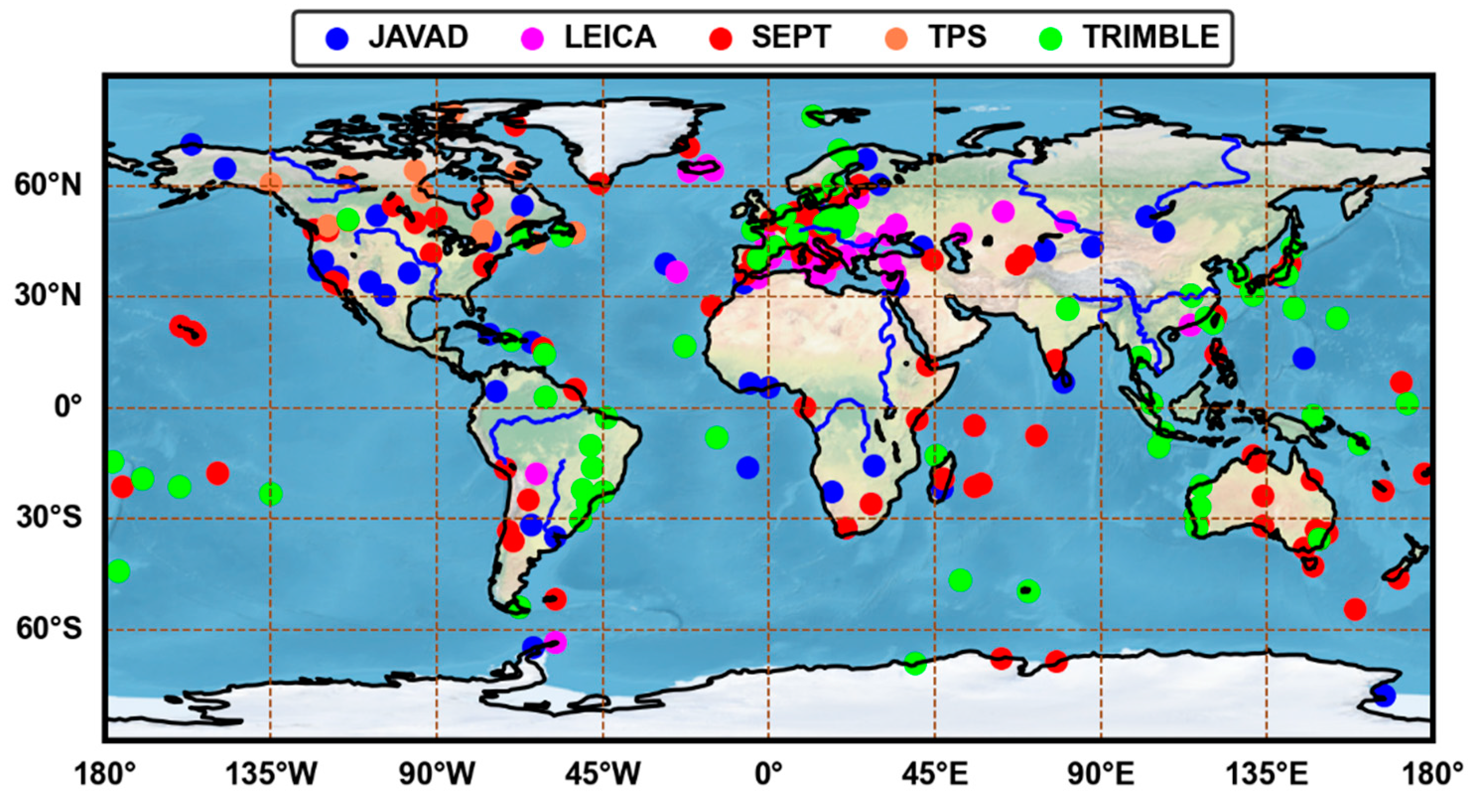
With the rapid development of the international GNSS service (IGS), a large number of GNSS stations are available. A collection of 302 stations from the MGEX, depicted in Figure 1, is used in this paper. The observations are downloaded from the IGS data center, during a period of a week from DOY 45 to 51, 2021. These stations, equipped with different types of receivers and antennas, are restricted to JAVAD, LEICA, Septentrio (SEPT) and TPS, as well as TRIMBLE. Additionally,

Table 1. Receiver types and the corresponding numbers.

Manufacturer	Hardware Type	Num
JAVAD	TR_G3TH	3
	TRE_3	10
	TRE_3 DELTA	29
	TRE_3N DELTA	4
	TRE_G3TH DELTA	22
LEICA	GR10	12
	GR25	7
	GR30	8
	GR50	15
SEPT	ASTERX4	6
	POLARX4TR	5
	POLARX5	68
	POLARX5TR	25
TPS	NET-G3A	7
	NET-G5	10
TRIMBLE	ALLOY	25
	NETR9	46

presents the details of the receiver hardware and firmware types.

Table 2. Signal types with RINEX v3.04 used for SDB analyses.

Manufacturer	GPS	Galileo	BDS
JAVAD	C1C C1W C2W	C1X C5X	C2I C6I
LEICA	C1C C2W	C1C C5Q	C2I C6I
SEPT	C1C C1W C2W	C1C C5Q	C2I C6I
TPS	C1C C2W	/	/
TRIMBLE	C1C C2W	C1X C5X	C2I C6I

depicts signal types with RINEX v3.04 for different receivers and GNSS systems. It should be noted that these receivers do not only track signal types listed in Table 2 and we just list the ones that we used for SDB analyses in this contribution. Meanwhile, not all receivers have been configured to track all signal types. For instance, only a part of JAVAD and LECIA receivers can track C6I signals for BDS. Besides, there are nearly 172 stations that can track BDS-3 signals and the maximum PRN is C46. It is noteworthy that most TRIMBLE NETR9 receivers can only track signals in a range from PRN C19 to C30 for BDS-3.

2.3.2. Analyses of the Characteristics of SDBs

Based on the method introduced above, PPP was performed to obtain SDB corrections in IF and MW combination forms for each station on a daily base. The details of data processing strategies are presented in

Table 3. Details of the data processing strategies.

Term	Description
Observation	Ionospheric-free combination
Cut-off elevation angle	$7°$
Sample rate	30 s
Antenna PCO and PCV	igs14.atx
DSB products	Products provided by CODE
BDS-2 elevation-related code bias	Corrected [26]
Tropospheric delay	Saastamoinen model + GMF mapping functions [27,28]
Satellite orbit and clock	GFZ MGEX final products GBM
Estimator	Square root information filter [29]
WL phase bias estimation	WL ambiguities from MW combination [12]
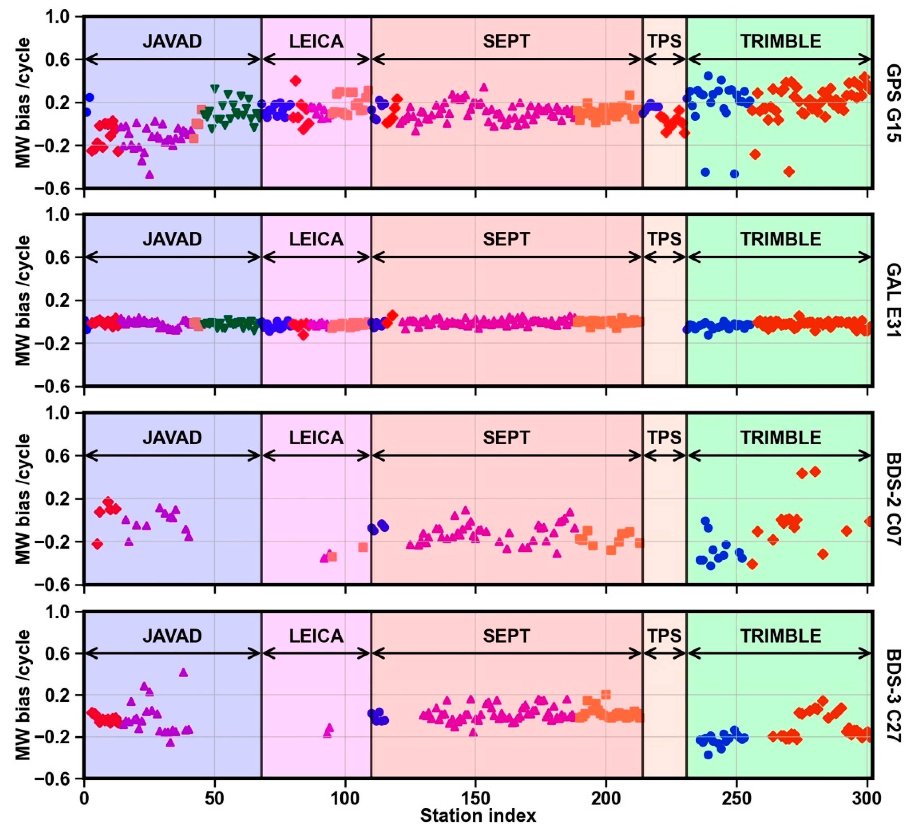
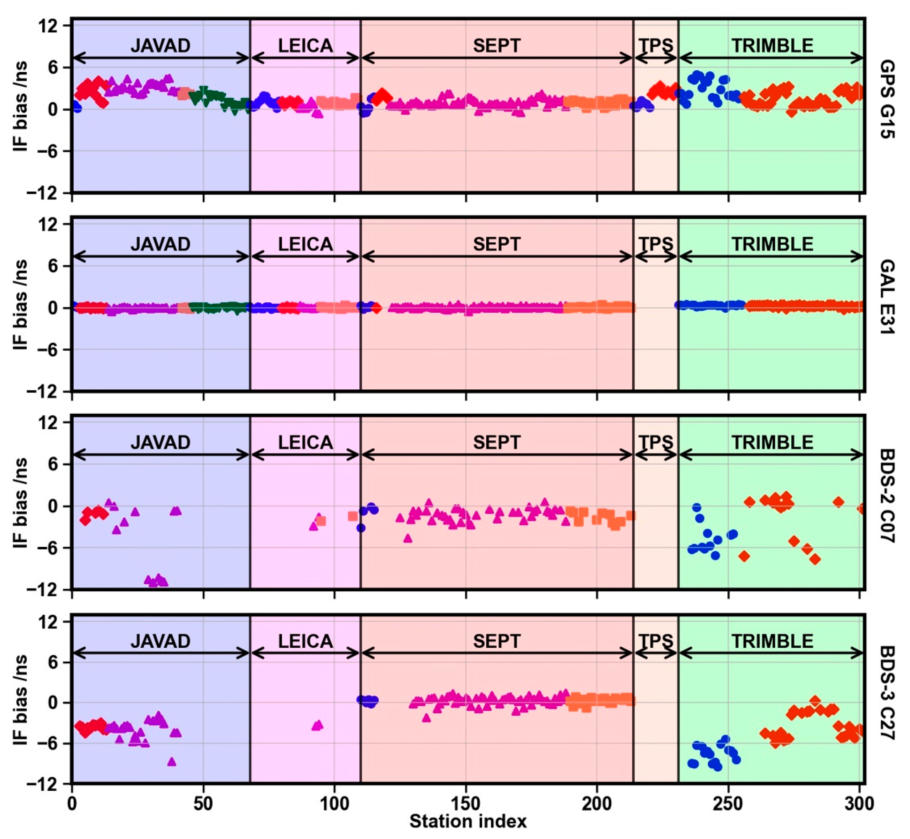
NL phase bias estimation	Using the IF ambiguity and fixed WL integer ambiguity [4]

. Considering that reference stations need have as many satellites as possible to observe, different reference stations were chosen for different systems. So, we selected stations ALGO, ALBH, SIN1 and KIRU for GPS, Galileo, BDS-2 and BDS-3 as reference stations, respectively. Thereafter, we obtained the daily MW and IF SDB corrections for each station and then averaged them from DOY 45 to 51, 2021. As presented in Figure 2 and Figure 3, the SDBs are divided into different groups. Different shapes and colors represent different hardware types.

Obviously, these SDBs are consistent with the receiver types. As shown in Figure 2 and Figure 3, we notice that the maximum SDBs for the MW combination can reach 0.66 cycles, while they can even reach 10 ns for the IF combination. There are few SDBs for Galileo, while a lot for GPS, BDS-2 and BDS-3. Furthermore, the same type of receiver responds differently to different systems. Some suggestions have been given that SDBs can be separated into different groups by manufacturers [17,19,22]. Nonetheless, for other systems except Galileo, the inconsistency also exists among receivers with identical hardware types or even versions. As presented in Figure 2 and Figure 3, JAVAD and TRIMBLE receivers have poor consistencies, and we cannot obtain corrections simply by categories. It is noteworthy that SEPT receivers remain in good consistencies for GPS, Galileo and BDS-3, while for BDS-2 in poor consistencies. Hence, we recommend that for GPS and BDS-3, all LEICA receivers be classified as one group, while all SEPT receivers, except SEPT ASTERX4, be divided into one group and all SEPT ASTERX4 receivers be classified into another group. Then, TPS receivers can be classified by hardware types, and each JAVAD and TRIMBLE receiver can correspond to one correction value. For Galileo, due to its excellent consistencies among receivers, they can simply be grouped by manufacturers. However, for BDS-2, due to its poor consistencies among receivers, we suggest that each receiver correspond to one correction value.

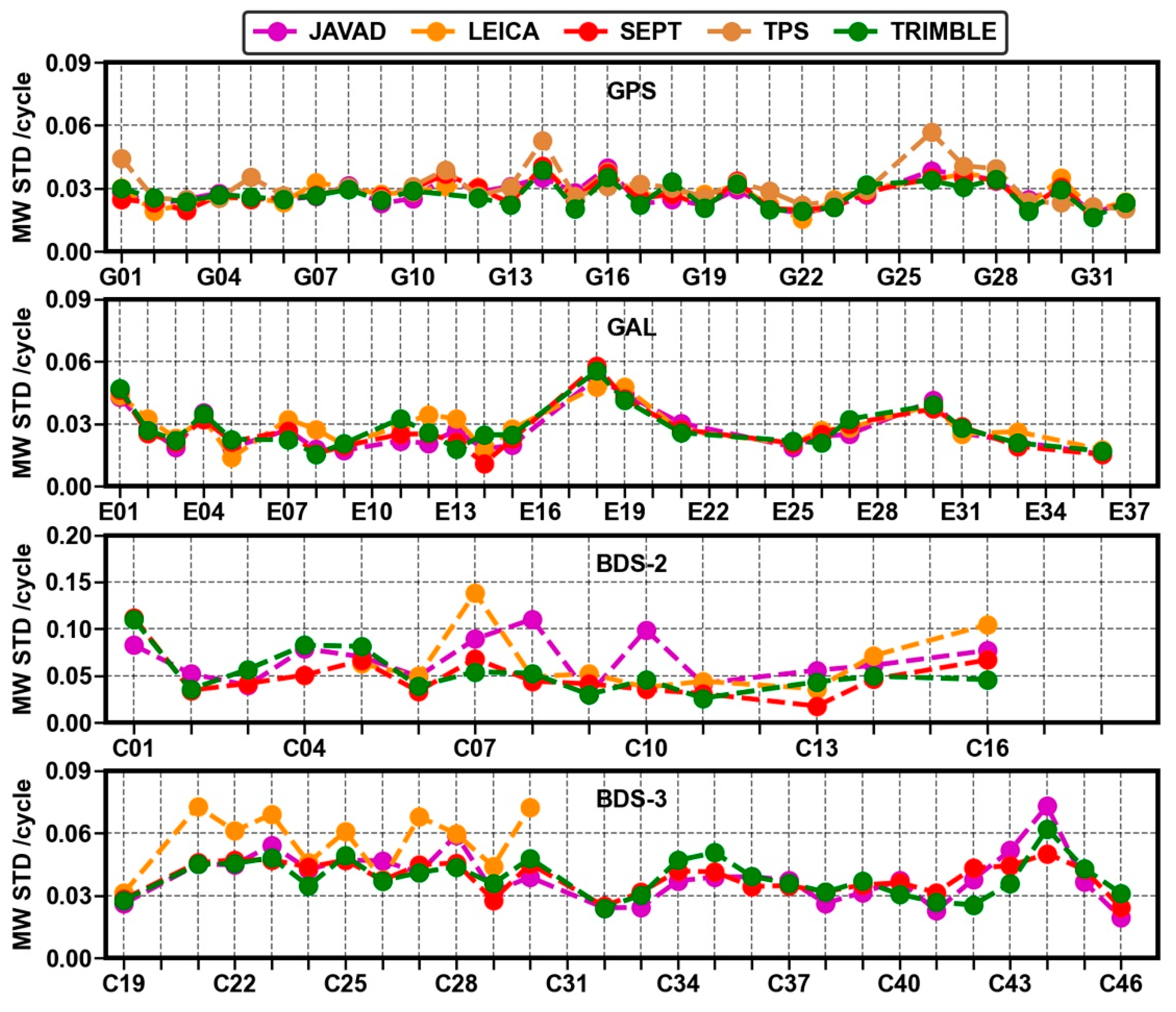
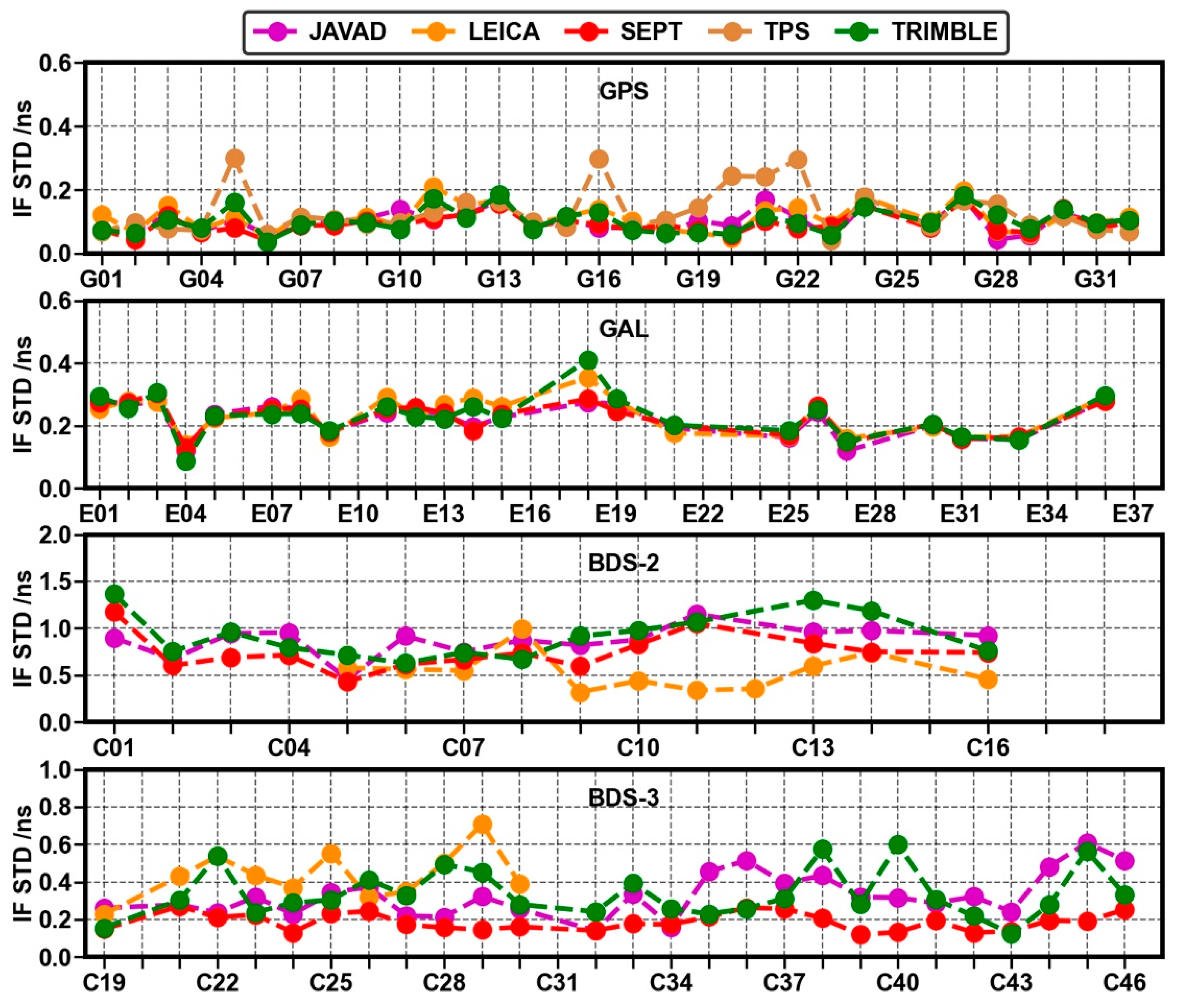
Regarding the stability of the SDBs, Figure 4 and Figure 5 show the average standard deviations (STDs) of the MW and IF SDBs across 7 days for GPS, Galileo, BDS-2 and BDS-3, respectively. In general, the SDBs are quite stable and can be further available for bias correction products. The STDs of the SDBs for GPS and Galileo are smaller than those for BDS. Additionally, the STDs of the IF SDBs are larger than those of the MW SBDs due to its larger noise amplification factor. It is noted that the comprehensive performance of SEPT receivers is the best among all types of receivers.

3. Experiments and Results

To compensate for SDBs among different types of receivers, we classified receivers as mentioned above, and took the average of the 7 daily biases as correction products. In this section, we applied the SDB corrections to WL and NL phase bias estimations and evaluated the performance from 4 aspects, including the consistency among different networks, the ambiguity fixing rates and the stability of phase bias series, as well as ambiguity residual distributions.

In this part, we first chose different networks and the corresponding reference receiver for different GNSS systems, respectively. Next, for the standard strategy (without SDB calibrations) and improved strategy (with SDB calibrations), we compared and evaluated their effects on phase bias estimation.

Considering the number and distribution, as well as the comprehensive performance of each type of receiver, we chose all SEPT receivers as a reference network. Other stations networks are presented in

Table 4. Network strategies of phase bias estimation.

System	Cases	Manufacturers	Number Available
GPS	Case 1	SEPT	104
	Case 2	TRIMBLE	71
	Case 3	TRIMBLE and JAVAD	139
Galileo	Case 1	SEPT	104
	Case 2	TRIMBLE	66
	Case 3	TRIMBLE and JAVAD	139
BDS-2	Case 1	SEPT	89
	Case 4	various types of receivers	134
BDS-3	Case 1	SEPT	89
	Case 3	TRIMBLE and JAVAD	79
	Case 4	various types of receivers	170

. Compared with GPS and Galileo, the number of stations available to track BDS-2/3 signals is smaller. Therefore, station networks for multi-system differ from each other.

3.1. WL Phase Bias Estimation

As analyzed in the previous section, the SDBs greatly affect the effectiveness of WL phase bias estimation based on the MW combination. Several experiments were carried out as follows.

3.1.1. The Consistency of Phase Bias Estimation among Different Networks

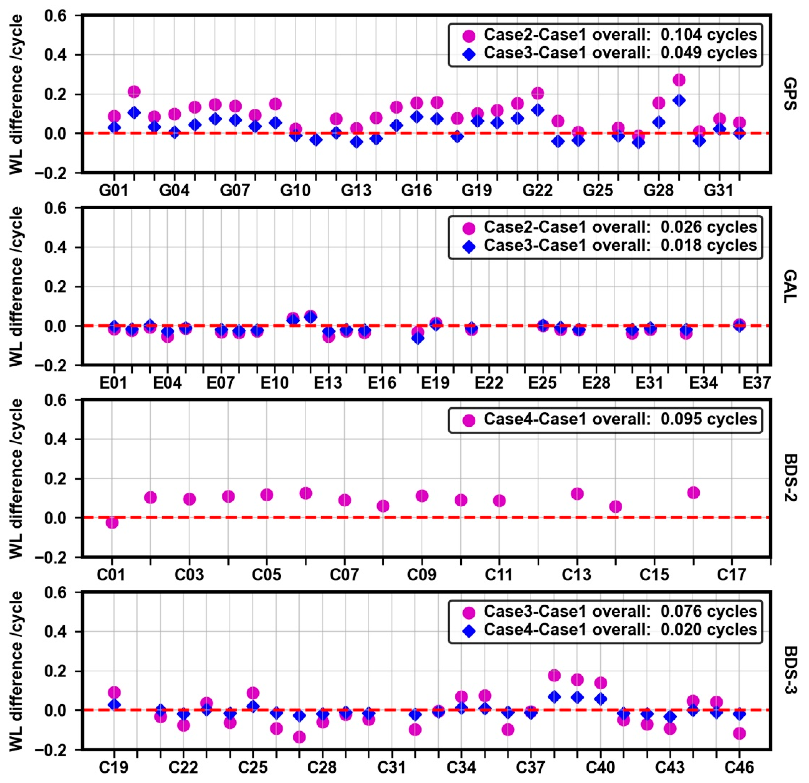
We estimated the daily phase biases with different networks from DOY 45 to 51, 2021 in total. Meanwhile, to remove systematic bias among different strategies, we selected G25, E24, C12 and C20 as reference datums, respectively. The characteristics of the satellite phase biases differences among different network strategies without the calibration, relative to Case 1, are presented in Figure 6. The overall deviation $d_{overall}$ of WL phase biases between different networks is determined as follows

$$d_{overall}=\frac{{\displaystyle \sum _{s=1}^n\left|d_{phase}^s\right|}}{n}$$

(12)

where $d_{phase}^s$ denotes satellite phase bias differences estimated between different networks with the unified benchmark; $n$ represents the valid number of satellites. $d_{overall}$ can reflect the overall degree of deviations among phase bias estimations from different networks, and if $d_{overall}$ is smaller, it demonstrates that the consistencies of phase bias products are better.

We notice that only Galileo shows the best agreement, and for GPS, BDS-2 and BDS-3, there are significant deviations between phase bias estimations among different networks. In Case 2, half of GPS satellites have deviations larger than 0.1 cycles, and the largest can even reach 0.26 cycles. The overall deviation of all GPS satellites is 0.104 cycles. In Case 3, consisting of TRIMBLE and JAVAD receivers, the deviations of GPS satellites decrease, but the overall deviation of all satellites still remains within 0.17 cycles. For Galileo, the deviations of all satellites are below 0.05 cycles and the overall deviations of the two strategies are 0.026 and 0.018 cycles, indicating excellent consistency among different receivers. For BDS-2, almost all the satellites have deviations close to 0.1 cycles, except the C01 satellite, and the overall deviation remains at 0.095 cycles. For BDS-3, there are five satellites with deviations larger than 0.1 cycles in Case 3. Additionally, the largest deviation among all satellites can even reach up to 0.18 cycles, and the overall deviation of all BDS-3 satellites is 0.076 cycles. When mixed types of receivers are used in Case 4, the deviations of almost all BDS-3 satellites decrease and are within 0.1 cycles.

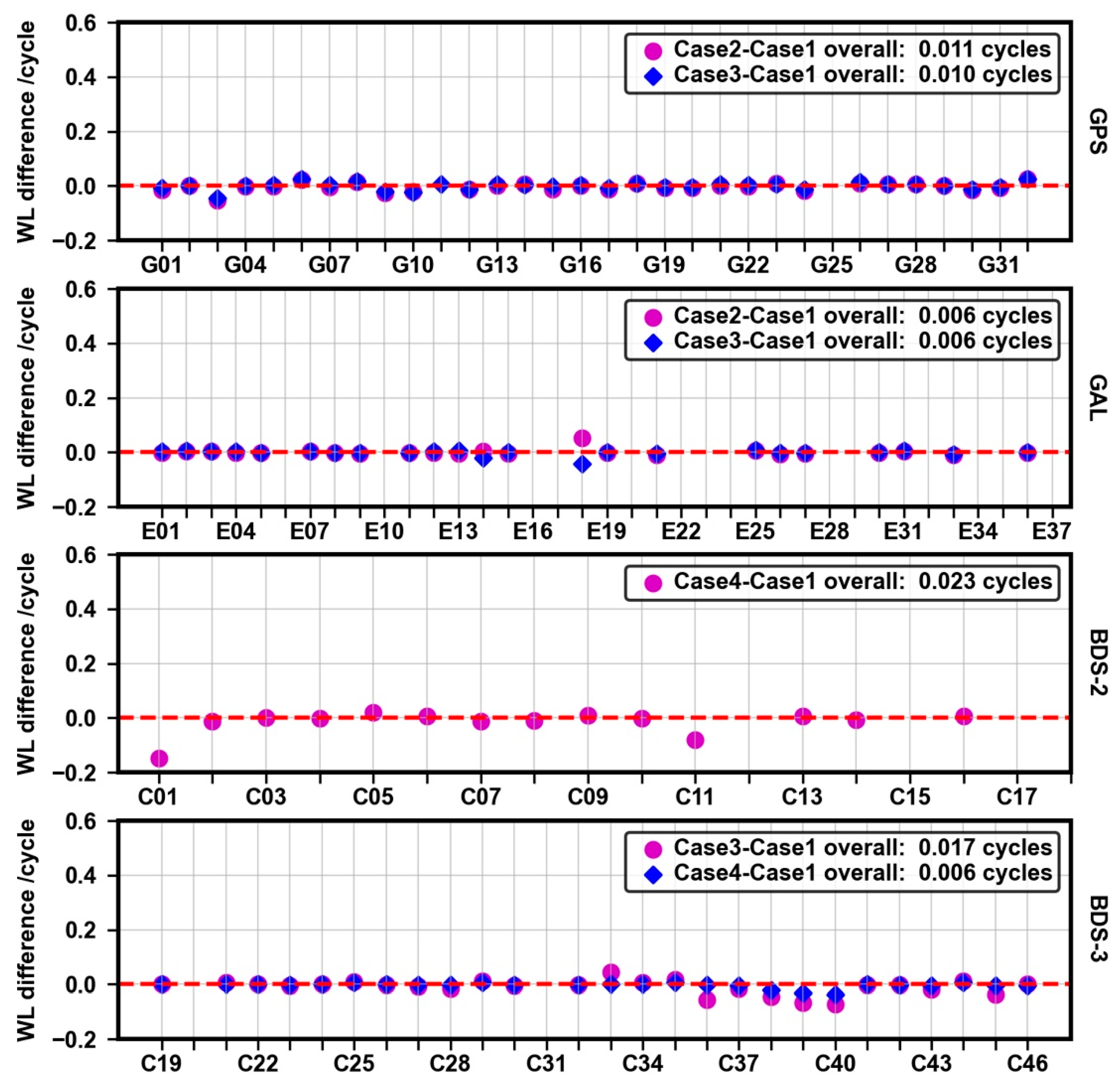
After applying the calibration, the performance of the improved case is presented in Figure 7. In Cases 2 and 3, the deviations of almost all GPS satellites are below 0.025 cycles. The overall deviations of the two cases are 0.011 and 0.010 cycles, respectively, with improvements of 89% and 80%. For Galileo, as mentioned before, it shows the best agreement and SDBs have limited influence on the WL phase bias estimation. However, the calibration still has a certain effect where the overall deviations are both reduced to 0.006 cycles for Cases 2 and 3, and improve by approximately 80% and 67%, respectively. For BDS-2, we notice that the deviations of almost all BDS-2 satellites, except C01 and C11 satellites, are with 0.02 cycles, and the overall deviation improves by approximately 76%, reduced to 0.023 cycles. For BDS-3, in Case 3, there are five satellites with a bias close to −0.05 cycles and other deviations basically approach zero. Additionally, it is obvious that in Case 4, the deviations of all BDS-3 satellites are near zero, showing the great performance of the calibration.

3.1.2. WL Ambiguity Fixing Rates

The WL phase bias estimation is performed, and in this experiment, the threshold of a fixing decision is simply set to ±0.1 cycles. The ambiguity fixing rate is determined as follow [19]:

$$P_{success, Type}=\frac{n_{fixed, Type}}{n_{all}}·100\%$$

(13)

where $n_{fixed, Type}$ denotes the number of WL or NL ambiguities fixed successfully; $n_{all}$ represents the number of all ambiguities involved in the calculation. In the following experiments, for brevity, we only chose Case 4 as a test network, equipped with mixed types of receivers.

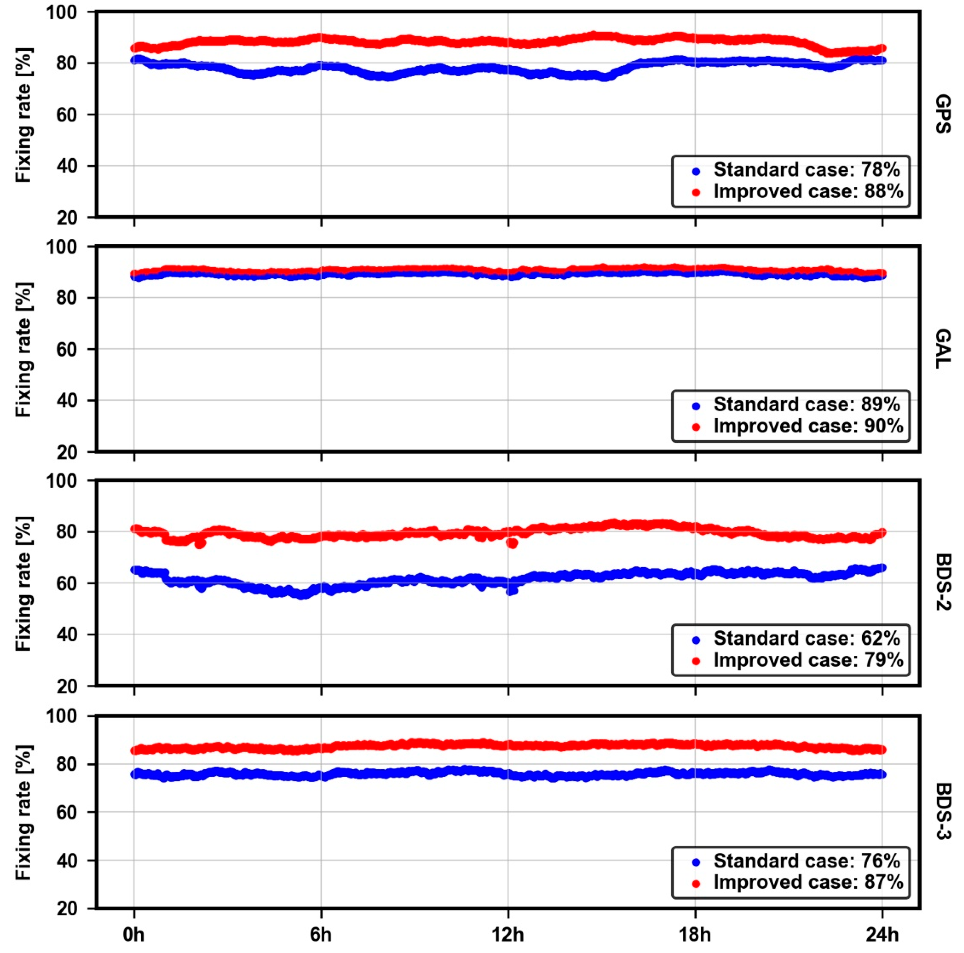
The seven-day average WL ambiguity fixing rates are presented in Figure 8. In general, after the calibration, the fixing rate of each system improves. For GPS, it is obvious that the fixing rate increases from 78% to 88%, an improvement of 13%. For Galileo, due to the excellent consistency among different receivers, the performance of the calibration is limited, but it still demonstrates an improvement of 1%. For BDS-2 and BDS-3, the fixing rates yield a massive improvement of approximately 27% and 14%, respectively.

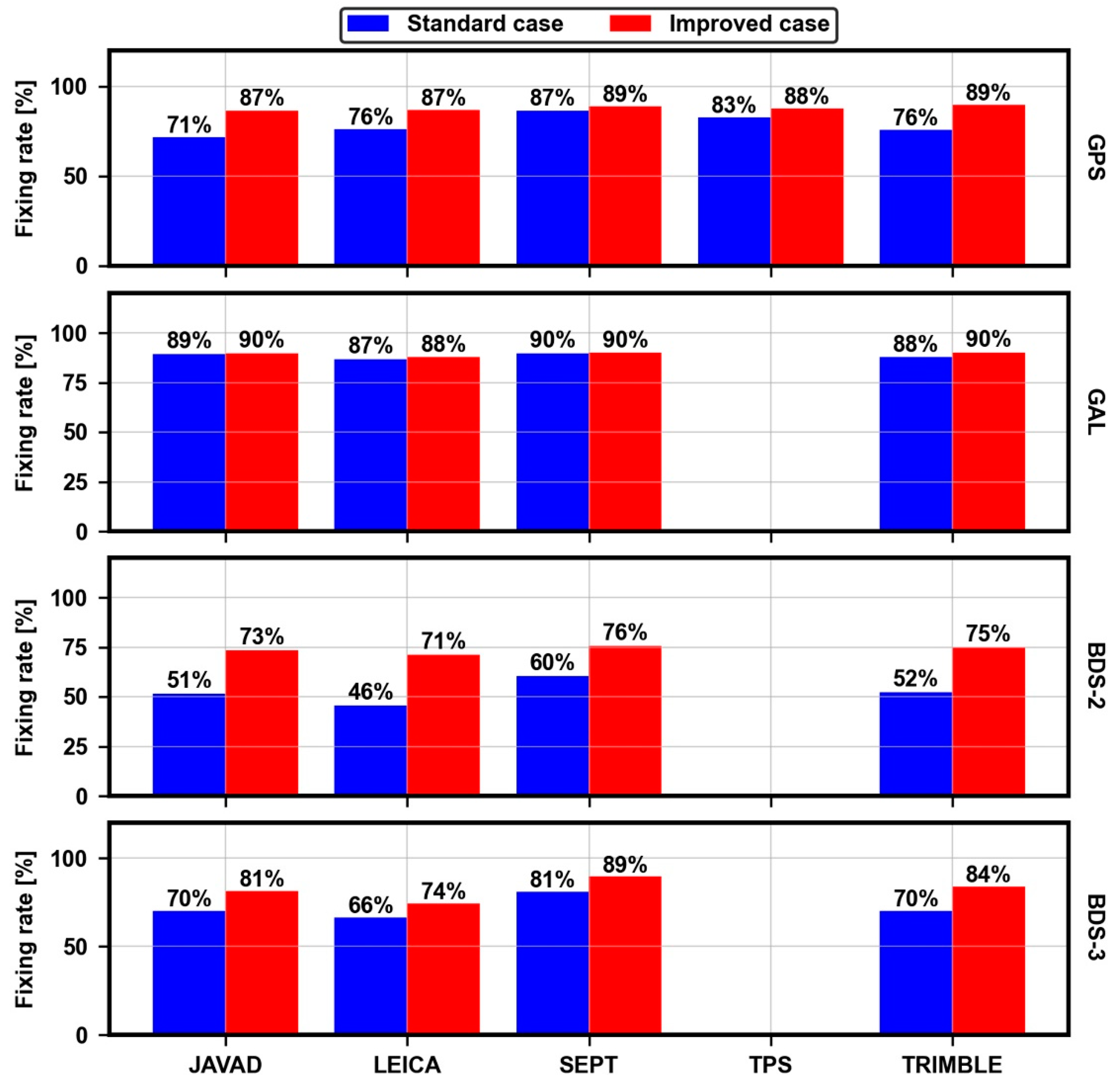
The WL ambiguity fixing rates of each receiver type for the standard case and improved case are shown in Figure 9. For GPS in the WL phase bias estimation without calibrations, the fixing rates of JAVAD, LEICA and TRIMBLE are below 76%, while those of other types, SEPT and TPS, reach more than 83%. After the calibration, the fixing rate of each type significantly improves, reaching more than 87%. Furthermore, the fixing rates of both JAVAD and TRIMBLE greatly improve by 23% and 17%, respectively. For Galileo, the performance of the calibration is not obvious for all types of receivers, where the maximum improvement is only 3%. For BDS-2, the fixing rate of each receiver type massively improves. The fixing rates of JAVAD, LEICA, SEPT and TRIMBLE for the standard case are 51%, 46%, 60% and 52%, respectively, while for the improved case reach 73%, 71%, 76% and 75%, respectively. For BDS-3, before the calibration, the overall fixing rate of each type is almost within 70%. After the calibration, the fixing rates of JAVAD, LEICA, SEPT and TRIMBLE reach 81%, 74%, 89% and 84%, respectively.

3.1.3. The Stability of WL Phase Bias Series

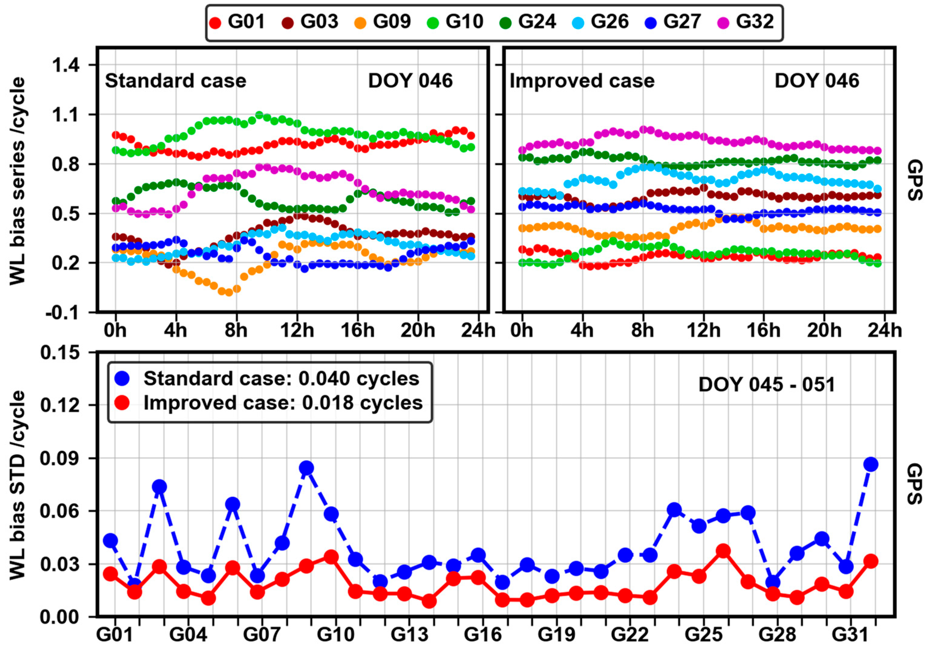
For brevity, we choose some GPS satellites randomly and their WL phase bias series on DOY 46, 2021 for the standard case and improved case are presented in half-hour intervals in Figure 10. Additionally, Figure 10 also depicts the average STDs of all GPS satellites across 7 days from DOY 45 to 51, 2021.

It is obvious that before the calibration, the stability of these GPS satellites chosen is significantly poor, and the maximum STD among GPS satellites is close to 0.08 cycles. After the calibration, these GPS satellites all show good stability, and the maximum STD is reduced to 0.038 cycles. In general, the calibration makes WL phase biases more stable, and the overall STD is reduced from 0.040 to 0.018 cycles, an improvement of approximately 55%.

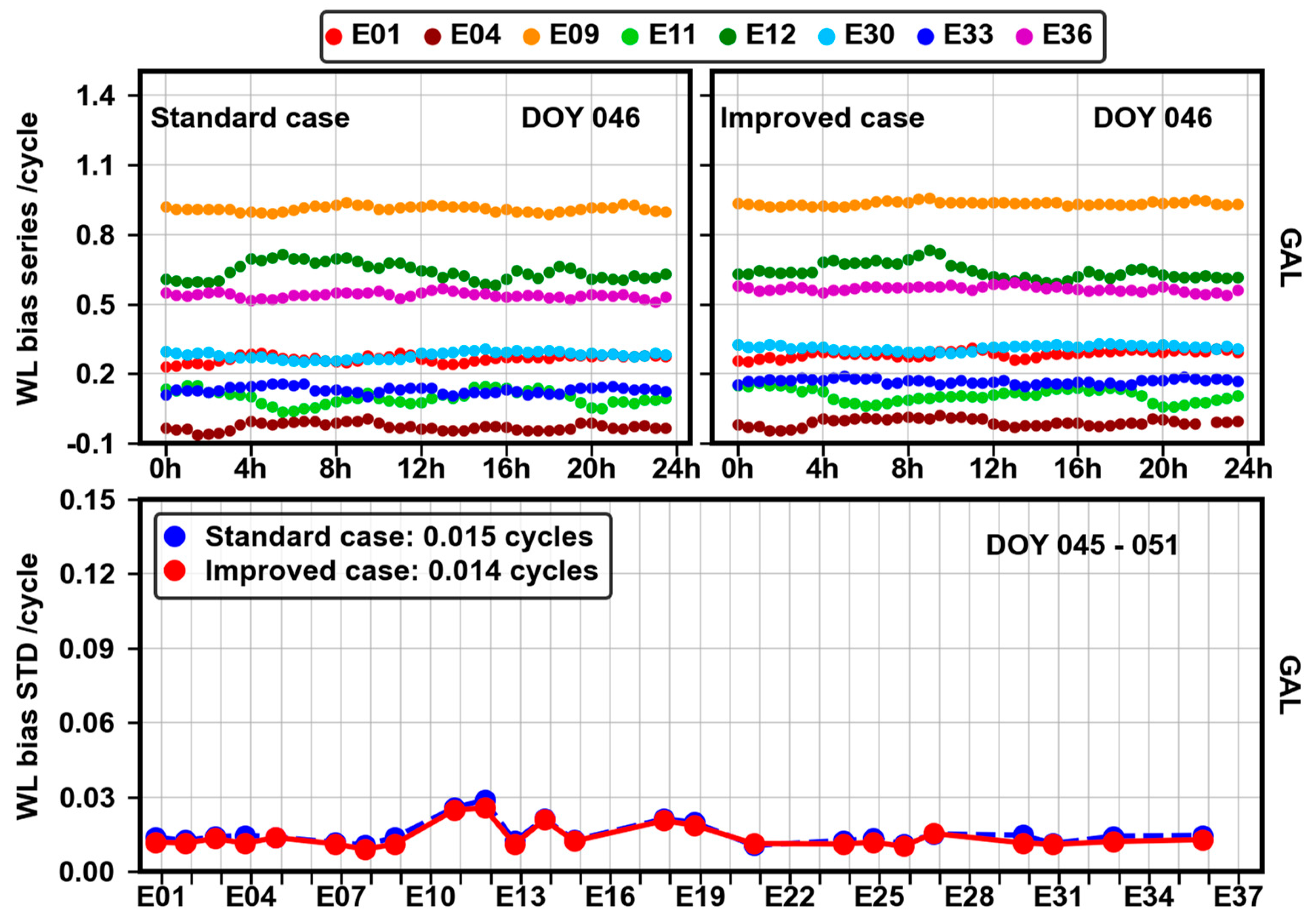
For Galileo, SDBs have limited impacts on the phase bias estimation. Regardless of whether the calibration is applied, Galileo WL phase bias series are significantly stable, and the overall STD is around 0.015 cycles, as presented in Figure 11.

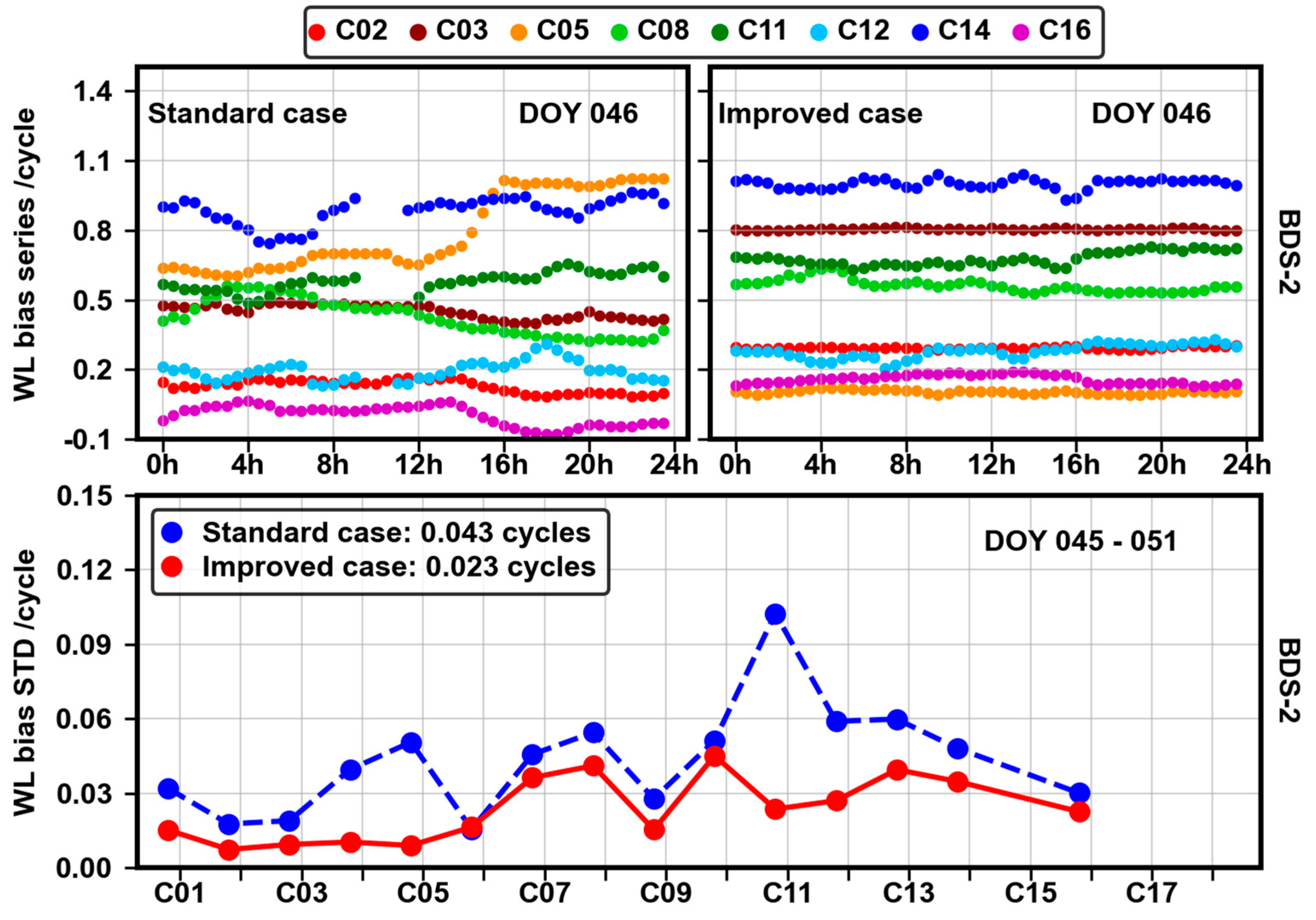
Figure 12 presents that before the correction, BDS-2 WL phase biases have the worst stability and the maximum STD among all satellites can reach 0.102 cycles. Even worse, these SDBs can cause the discontinuity in WL phase bias series, as the C11 and C14 satellites show. After the calibration, all BDS-2 satellites are in good stability and their discontinuities of the WL phase bias series are eliminated. Additionally, the STDs of all satellites are within 0.046 cycles and the overall STD has an improvement of 47%.

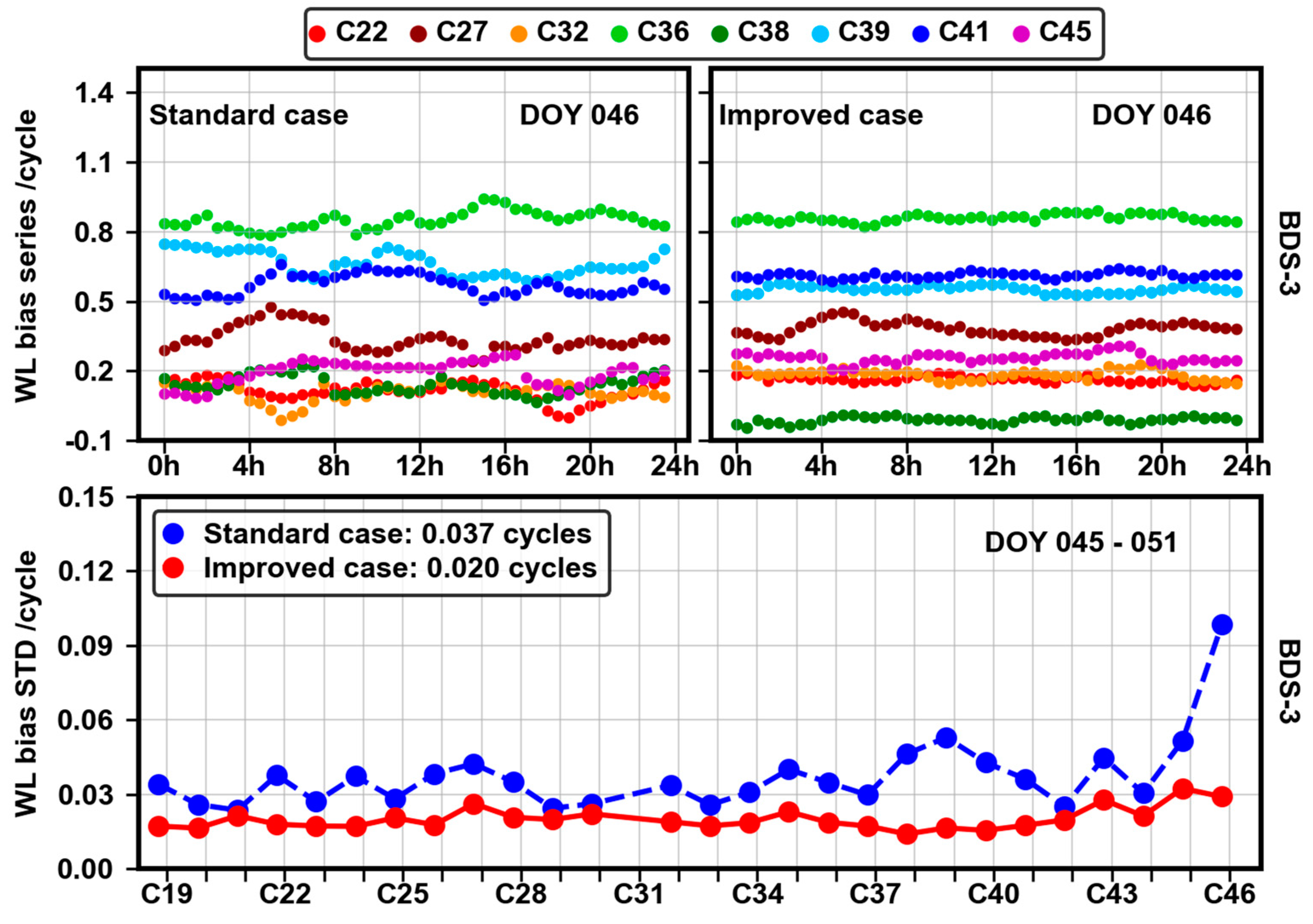
As shown in Figure 13, the maximum STD among BDS-3 satellites reaches 0.1 cycles. It is obvious that after the calibration, the BDS-3 WL phase bias series can become relatively smooth, and the STDs of all satellites are within 0.032 cycles. Furthermore, the average STD is reduced from 0.037 to 0.020 cycles, an improvement of approximately 46%.

In general, before the calibration, except for Galileo, WL phase biases for the other systems are almost in poor stability and, even worse for BDS-2, there might be some discontinuities in the WL phase bias series. However, when the calibration is applied, their WL phase bias stability improves greatly, and the corresponding discontinuities are eliminated.

3.1.4. Residual Distributions

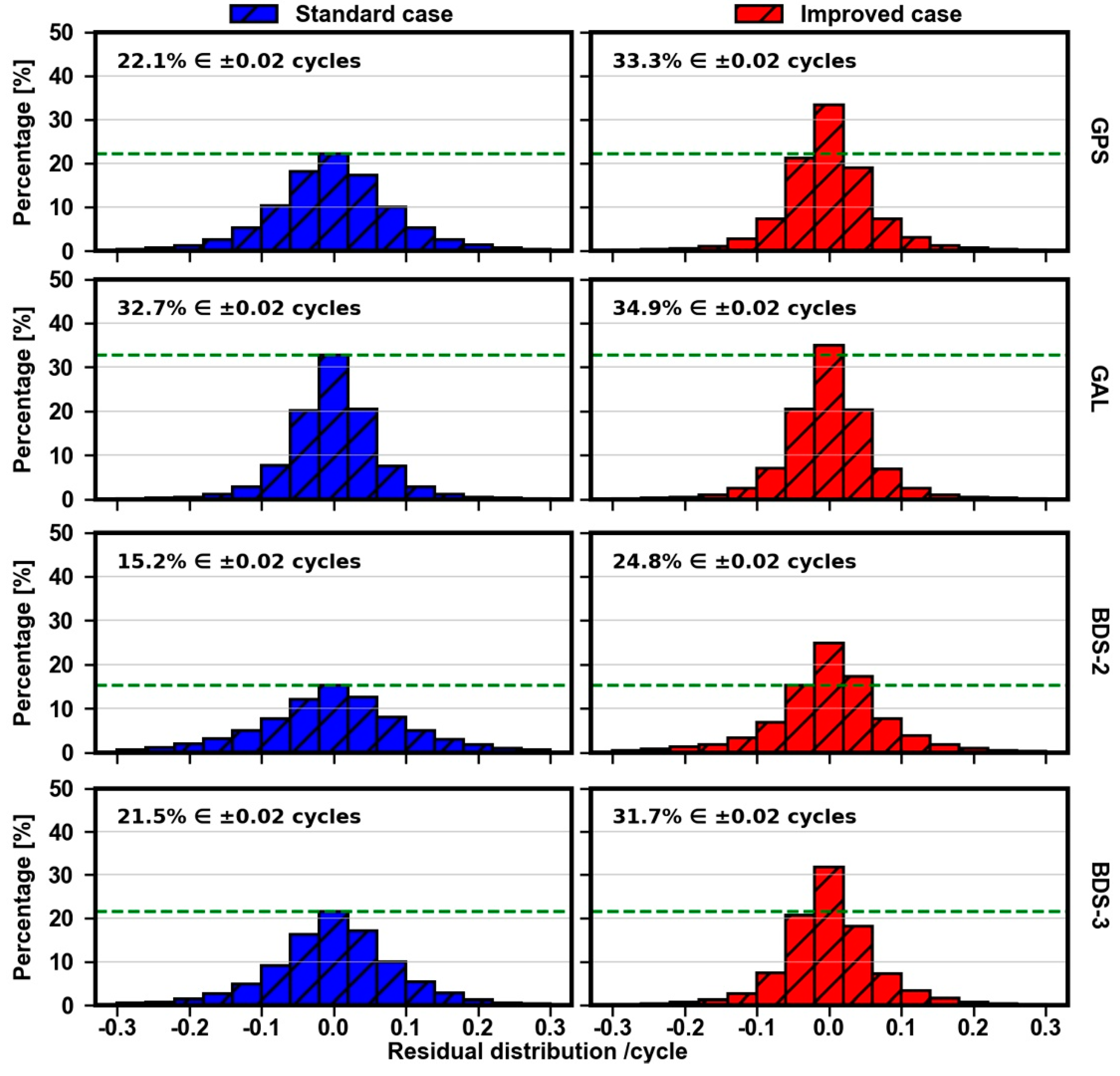
The residual distributions of WL ambiguities for the standard case and improved case, presented in Figure 14, can reflect the quality of phase bias estimation. For GPS, before the calibration, residuals within ±0.02 cycles only account for 22.1%, and there are quite a few residuals distributed in ranges beyond ±0.1 cycles. After the calibration, the number of residuals within ±0.02 cycles are larger, accounting for 33.3%. For Galileo, the calibration has a limited impact. Residuals within ±0.02 cycles before and after the calibration account for 32.7% and 34.9%, respectively. Additionally, regardless of whether the calibration is applied, almost all residuals are concentrated in ranges within ±0.1 cycles. For BDS-2, after the calibration, the proportion of residuals within ±0.02 cycles improve from 15.2% to 24.8%. Furthermore, the number of residuals beyond ±0.1 cycles decrease greatly. For BDS-3, before the calibration, residuals within ±0.02 cycles account for 21.5% and there are still a few residuals distributed in ranges beyond ±0.1 cycles. However, after the calibration, the proportion of residuals within ±0.02 cycles improve greatly, reaching 31.7%.

3.2. NL Phase Bias Estimation

The NL phase bias estimation is related to satellite clock and DSB products, while the SDBs are ignored in the existing products. In this paper, the SDB corrections in Section 3 actually absorb the deviations of satellite DSBs and can directly eliminate the impacts on satellite DSBs. Nonetheless, the deviations of satellite clocks cannot be simply dealt with. To eliminate the effect of the SDBs on the satellite clocks, we must recalculate the satellite clocks with the calibration of these SDBs. Then, based on the products re-estimated, the performance of NL phase bias estimation is evaluated. Here we adopt the FUSING software for the satellite clock estimation, for the detailed information of satellite clock estimation, we refer to [30].

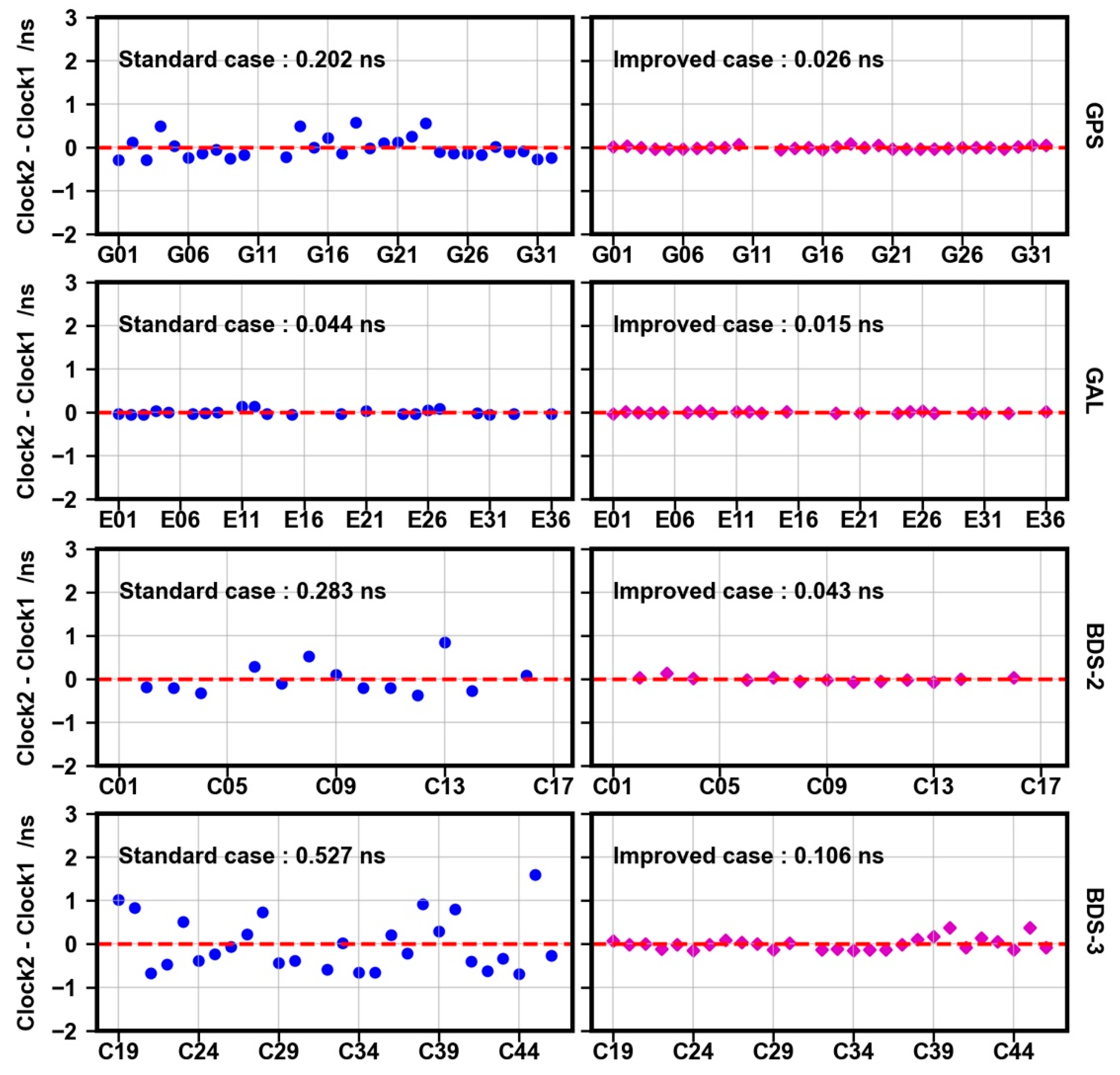
As presented in

Table 5. Processing strategies of satellite clock estimation.

Clock Cases	Manufacturers	Available Number
Clock 1	SEPT	104
Clock 2	Mixed types of receivers, including JAVAD, LEICA, SEPT, TPS and TRIMBLE	120

, two different networks are chosen to estimate the satellite clocks. One of them, consisting of all SEPT receivers, is selected as the reference product, and the other consists of mixed types of receivers. We took the average satellite clock differences relative to Clock 1, presented in Figure 15. To remove systematic bias, we aligned the results to the average satellite clock for each GNSS system.

In general, satellite clocks are greatly influenced by these SDBs. For GPS, the maximum of clock differences without the calibrating can reach 0.583 ns, while with the calibrating, the maximum decreases to 0.082 ns. Additionally, the average clock difference decreases from 0.202 to 0.026 ns, an improvement of 87%. For Galileo, the impact of SDBs is limited. Regardless of whether the calibration is applied, the clock differences of all satellites are close to zero. However, the average clock difference still yields an improvement of 66%. For BDS-2, the satellite clock differences are larger than those of GPS and Galileo. The maximum can reach 0.841 ns and the overall clock difference is approximately 0.283 ns before the calibration. After the calibration, the overall clock difference yields an improvement of approximately 85%. For BDS-3, the maximum among satellite clock differences before the calibration reaches 1.587 ns, while approximately 0.383 ns after the calibration. The overall clock difference decreases from 0.527 to 0.106 ns, an improvement of 80%.

3.2.1. The Consistency of Phase Bias Estimation among Different Networks

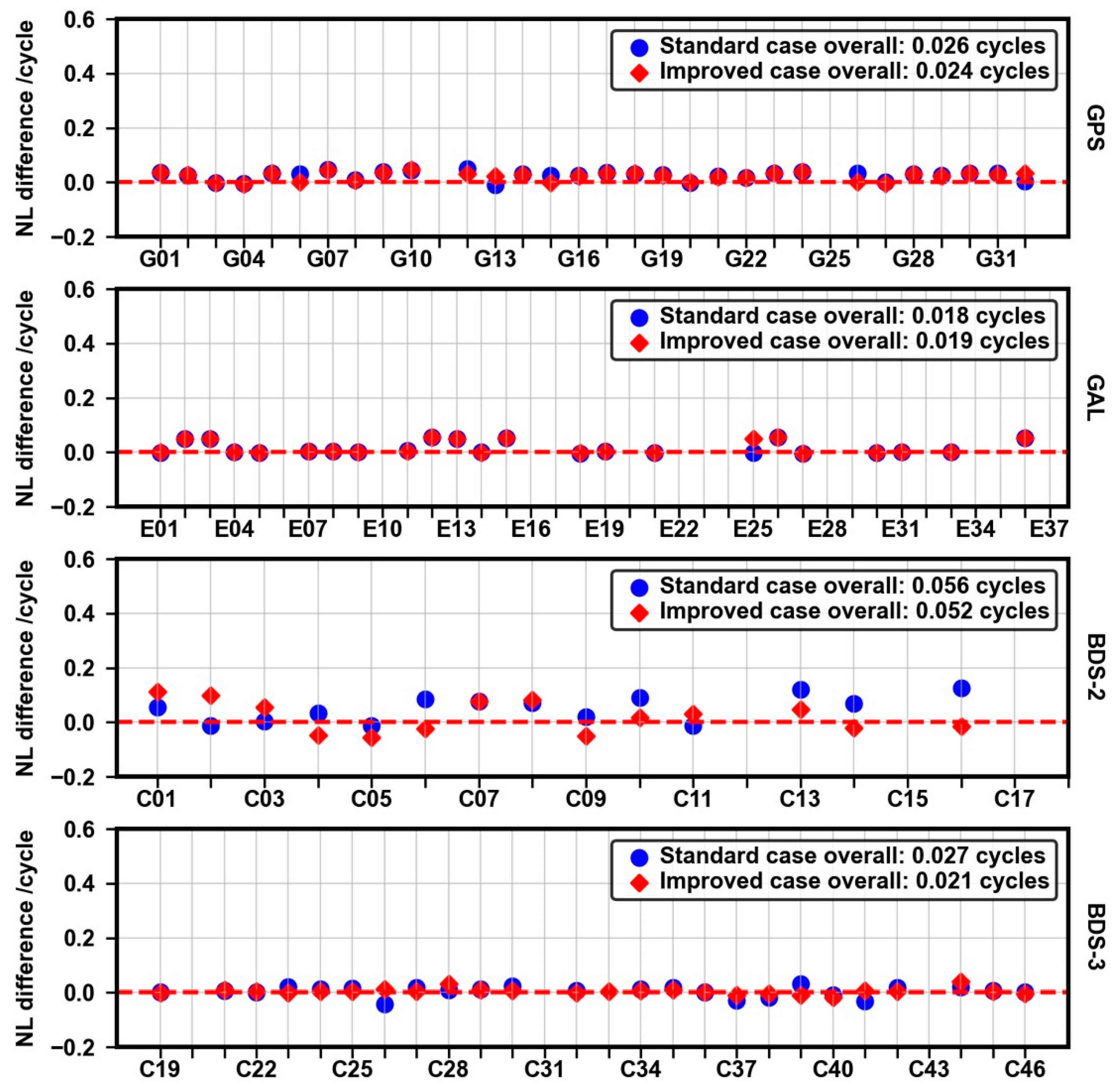
We selected Cases 1 and 4, listed in Table 4, and calculated the NL phase bias differences between the two cases for the standard case and improved case. G25, E24, C12 and C20 are chosen as reference satellites for GPS, Galileo, BDS-2 and BDS-3, respectively.

Figure 16 plots the characteristics of the satellite phase bias differences of different networks relative to Case 1 for the standard case and improved case. NL phase bias differences for each GNSS system except BDS-2 exhibit few deviations. For BDS-2, although a few satellites exhibit deviations close to 0.1 cycles, the overall NL difference remains within 0.056 cycles and it does not change much before and after the calibration. Therefore, we concluded that these SDBs do not influence the consistency of NL phase biases.

3.2.2. Ambiguity Fixing Rates

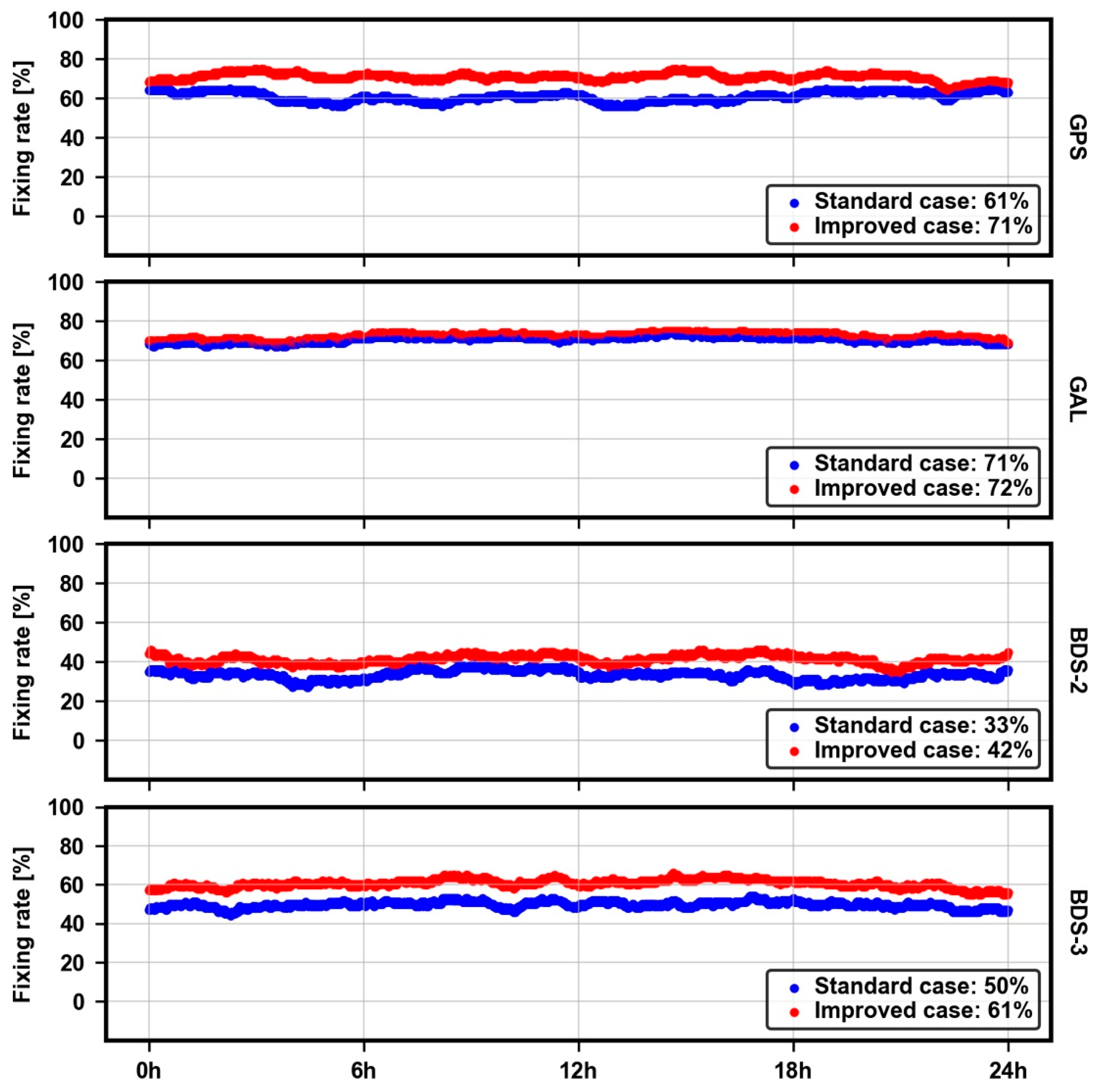
From an inhomogeneous network Case 4, we calculated the seven-day average NL ambiguity fixing rates for each GNSS system for the standard case and improved case. The threshold of a fixing decision for NL ambiguities is the same as WL ambiguities, which is simply set to ±0.1 cycles.

According to Equation (13), the NL ambiguity fixing rates across seven days are calculated, which are depicted in Figure 17. For GPS, after the calibration, the NL overall fixing rate increases from 61% to 71%. For Galileo, there is rarely no improvement. For BDS-2, the calibration makes the fixing rate reach 42%, while it only reaches 33% without SDB calibrations. Ultimately, for BDS-3, the calibration still works, which can make the fixing rate increase form approximately 50% to 61%.

3.2.3. The Stability of NL Phase Bias Series

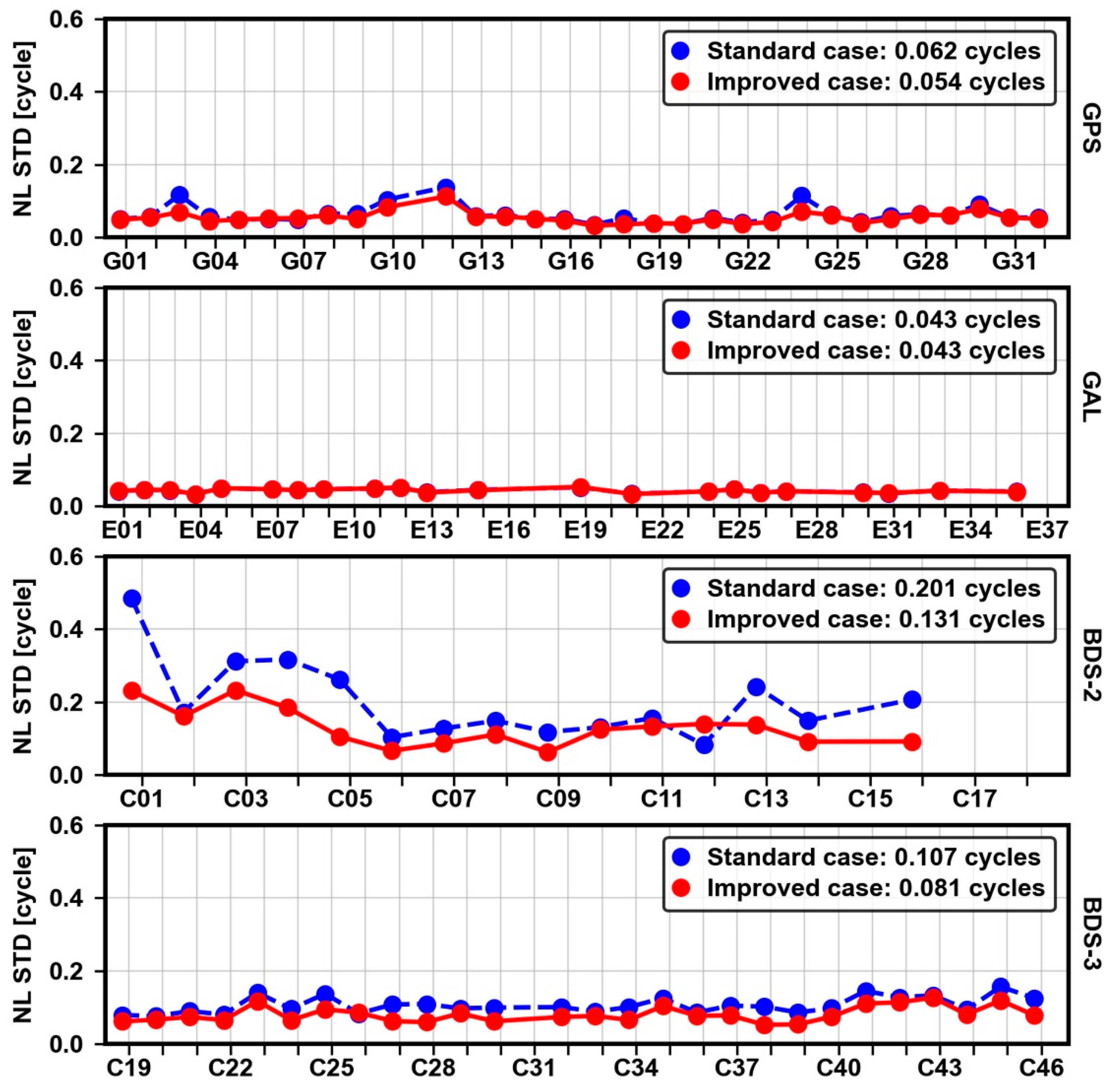
Considering that the temporal changes of NL phase bias series are relatively large, it is difficult to compare the temporal diagrams directly. Therefore, we calculated and compared the average STDs of NL phase bias series from DOY 45 to 51, 2021.

Figure 18 depicts the STDs of the NL phase bias series without and with the calibration. In general, each system, except BDS-2, has good stability. Before the calibration, the overall average STDs of NL phase bias series for GPS and Galileo are within 0.062 cycles, while close to 0.11 cycles for BDS-3. For BDS-2, the stability of the NL phase bias series is relatively poor, and the overall average STD can reach 0.201 cycles. Especially for some BDS-2 satellites, the STDs of the NL phase bias series exceed 0.3 cycles. The reason is that the fixing number for BDS-2 is relatively small, and it causes the discontinuity in NL phase biases. After the calibration, the overall average STD for GPS is reduced from 0.062 to 0.054 cycles, an improvement of approximately 13%. For Galileo, the improvement of the calibration is small. Because the increase in the NL ambiguity fixing number is sufficiently small, thus limiting the effect. For BDS-2, after the calibration, the overall average STD of the NL phase bias series is reduced to 0.131cycles, an improvement of approximately 35%. Similarly, for BDS-3, the overall average STD decreases from 0.107 to 0.081 cycles, an improvement of 24%.

3.2.4. Residual Distributions

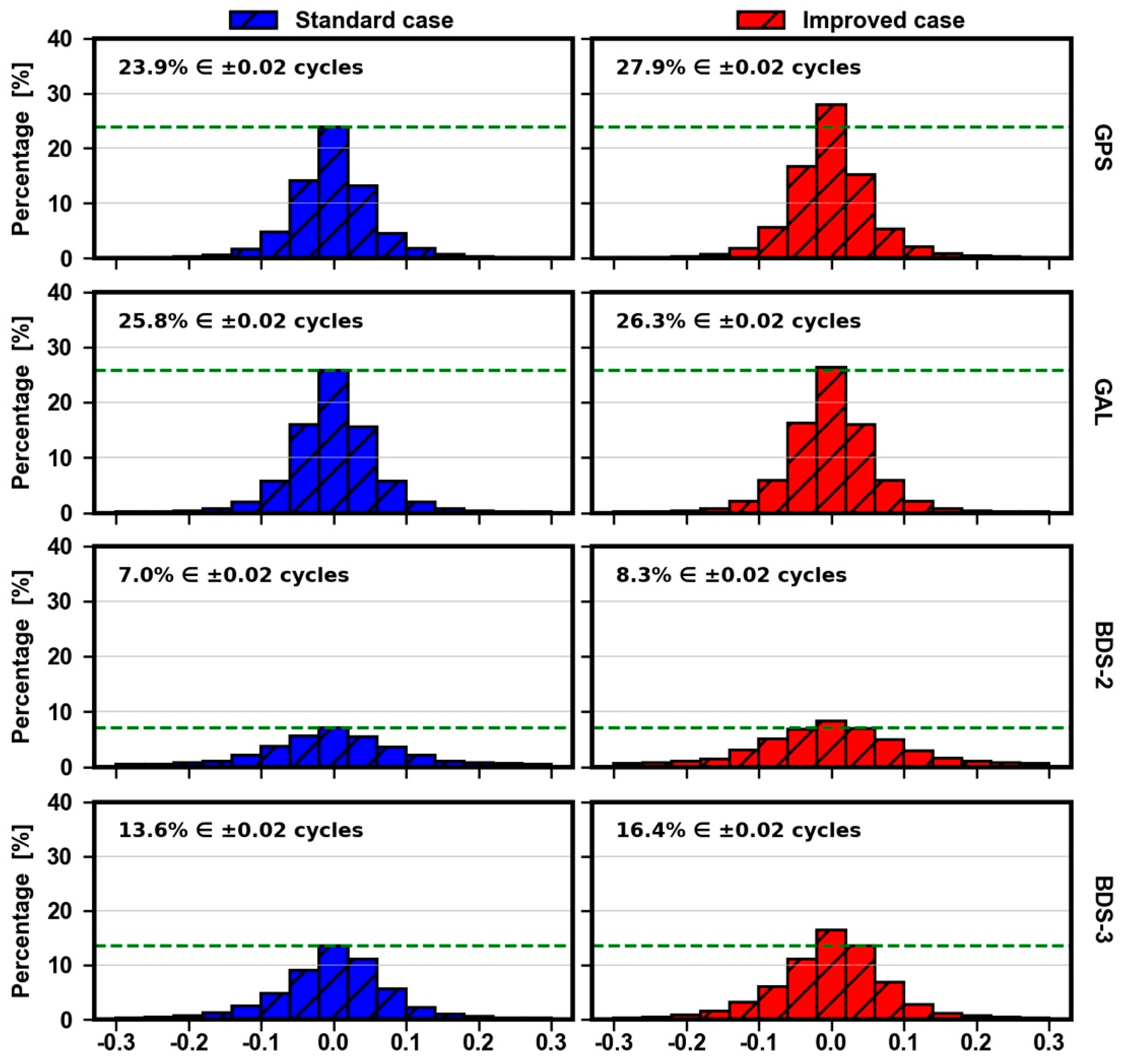
The residual distributions of NL ambiguities for the standard case and improved case are depicted in Figure 19. For GPS, after the calibration, the proportion of NL ambiguity residuals with ±0.02 cycles increases from 23.9% to 27.9%, which yields an improvement of 17%. Additionally, more residuals are concentrated in ranges within ±0.1 cycles. For Galileo, the performance of the calibration is not obvious, and the increase of residuals within ±0.02 cycles is little. For BDS-2, after the calibration, the number of ambiguity residuals within ±0.02 cycles improves by approximately 19%, accounting for 8.3%. Similarly, for BDS-3, after the calibration, the proportion of NL ambiguity residuals which are concentrated in ranges within ±0.02 cycles can account for 16.4% and improve massively by 21%. In addition, the number of ambiguity residuals beyond ±0.1 cycles decreases, which reflects that the corresponding ambiguity fixing rate improves.

4. Discussion

Receiver-related SDBs play an important role in precise data processing and recently some research has been carried out. However, there is no comprehensive and systematic study for WL and NL phase bias estimations.

In this contribution, an experimental validation has been carried out with 302 stations from the MGEX, including JAVAD, LEICA, SEPT and TPS, as well as TRIMBLE receivers. GPS C1C, C1W and C2W signals, Galileo C1X, C1C, C5X and C5Q signal, and BDS C2I and C6I signals are used to analyze SDBs among 5 manufacturers. We find that these SDBs which can reach 0.66 cycles and 10 ns for MW and IF combination cannot be ignored. Meanwhile, we notice that SDBs are stable during a period of time, and they can be further applied to calibrate relevant biases to improve phase bias estimation.

The experiment demonstrates that these SDBs are related to receiver types. The responses from SDBs of different receiver types to different GNSS systems differ from each other. Among them, SDBs for Galileo are significantly smaller and have limited impacts. Nonetheless, other GNSS systems show larger SDBs, and SDBs for BDS-3 are relatively smaller than those for BDS-2, as well as their impacts. In addition, among all types of receivers, we notice that SPET receivers show the best consistency and performance. Therefore, we suggest that the corresponding corrections are not simply classified by manufacturers or hardware types and that the classification depend on the specific performance of each receiver type for each GNSS system. This differs from other scholars’ research. First, considering excellent consistencies among different types of receivers for Galileo, it is appropriate that the SDB corrections can be directly grouped by manufacturers. Next, for GPS and BDS-3, all LEICA receivers and all SEPT receivers, except SEPT ASTERX4, should be divided into two groups, while SEPT ASTERX4 receivers should form one group. According to hardware types, TPS receivers can be grouped directly. Due to the particularly wide variation between JAVAD receivers, each JAVAD receiver needs to correspond to one correction, as do TRIMBLE receivers. Ultimately, considering BDS-2, no matter for which type of receivers, the differences between them are significant, and it is appropriate and necessary that each receiver needs to correspond to one correction for BDS-2.

The experimental results from DOY 45 to 51, 2021 demonstrate that the SDBs yield great impacts on phase bias estimation. After SDB calibrations, WL phase bias differences among different networks for GPS, Galileo, BDS-2 and BDS-3 decrease by approximately 89%, 77%, 76% and 78%, respectively. In addition, the WL ambiguity fixing rates for GPS, BDS-2 and BDS-3 improve significantly by 13%, 27% and 14%, respectively, while for Galileo, due to its small SDBs, it only yields a slight improvement. With improvements of WL ambiguity fixing rates, the NL ambiguity fixing rates further improve. Similar to WL ambiguities, there is scarcely any improvement for Galileo, while for GPS, BDS-2 and BDS-3 they show great improvements of 16%, 27% and 22%, respectively. On the other hand, applying the calibration can make phase bias series more stable and ambiguity residuals more concentrated. The STDs of WL phase bias series for GPS, Galileo, BDS-2 and BDS-3 improve by approximately 55%, 7%, 47% and 46%, respectively, while those of NL phase bias series for GPS, BDS-2 and BDS-3 improve by approximately 13%, 35% and 24%, respectively. As for the residual distributions, after the calibration, more WL and NL ambiguity residuals are concentrated in ranges within ±0.02 cycles. The improvements of WL ambiguity residuals within ±0.02 cycles for GPS, Galileo, BDS-2 and BDS-3 can reach approximately 51%, 7%, 63% and 47%, respectively, while those of NL ambiguity residuals can reach approximately 17%, 2%, 19% and 21%, respectively.

5. Conclusions

Due to the difference of the correlator and the front-end design among different types of receivers, receiver related SDBs exist, which has great importance in GNSS precise data processing. In this contribution, based on a large data set from the MGEX network, we analyze the characteristics of SDBs and obtain the corresponding corrections by the calibration method proposed, and further apply them to WL and NL phase bias estimations.

We evaluate the effects of SDBs on WL and NL phase bias estimations and the performance of SDB calibration methods from several aspects. This research proves that there are few effects for Galileo, but there is a significant influence for GPS and BDS. Besides, to some extent, for PPP-AR on the user side, the SDBs are also supposed to be considered. Such biases of PPP users should consist of phase bias estimation and if not calibrated, the ambiguity fixing will also be affected.

Ultimately, based on the results of this work and other relevant research, it should be noted that SDBs must be taken into account and calibrated when inhomogeneous stations are used in future work.