Improving Leaf Area Index Retrieval Using Multi-Sensor Images and Stacking Learning in Subtropical Forests of China

Abstract

The leaf area index (LAI) is a key indicator of the status of forest ecosystems that is important for understanding global carbon and water cycles as well as terrestrial surface energy balances and the impacts of climate change. Machine learning (ML) methods offer promising ways of generating spatially explicit LAI data covering large regions based on optical images. However, there have been few efforts to analyze the LAI in heterogeneous subtropical forests with complex terrain by fusing high-resolution multi-sensor data from the Sentinel-1 Synthetic Aperture Radar (SAR), Sentinel-2 Multi Spectral Instrument (MSI), and Advanced Land Observing Satellite-1 digital elevation model (DEM). Here, forest LAI mapping was performed by integrating the MSI, SAR, and DEM data using a stacking learning (SL) approach that incorporates distinct predictions from a set of optimized individual ML algorithms. The method’s performance was evaluated by comparison to field forest LAI measurements acquired in Xingguo and Gandong of subtropical China. The results showed that the addition of the SAR and DEM images using the SL model compared to the inputs of only optical images reduced the mean absolute error (MAE) and root mean square error (RMSE) by 26% and 18%, respectively, in Xingguo, and by 12% and 8%, respectively, in Gandong. Furthermore, the combination of all images had the best prediction performance. SL was found to be more robust and accurate than conventional individual ML models, while the MAE and RMSE were decreased by 71% and 64%, respectively, in Xingguo, and by 68% and 59%, respectively, in Gandong. Therefore, the SL model using the three-source data combination produced satisfied prediction accuracy with the coefficients of determination (R²), MAE, and RMSE of 0.96, 0.17, and 0.28, respectively, in Xingguo and 0.94, 0.30, and 0.47, respectively, in Gandong. This study revealed the potential of the SL algorithm for retrieving the forest LAI using multi-sensor data in areas with complex terrain.

1. Introduction

Subtropical forests cover approximately 26% of China’s land area and play an important role in preserving plant and animal biodiversity, regulating terrestrial carbon cycles, preventing land degradation, and fostering regional and global ecological balance [1,2,3]. From the 1950s to the 1990s, soil erosion, wildfires, deforestation, and over-cultivation led to severe forest degradation in southern China [4]. To reverse this trend, China initiated a Grain-for-Green Project in the late 20th century [5]. As a result, forests in this region have been restored and vegetation cover and productivity have gradually increased [6]. Monitoring forest dynamics requires precise measurement of the spatial and geographical distributions of forest biophysical characteristics [7]. The leaf area index (LAI), defined as one-half of the total leaf area per unit ground area, is a vital physiophysical parameter for characterizing forest structure because it is used to estimate forest biomass, health, longevity, and productivity [8]. Additionally, the LAI is a key input for the ecosystem-level modeling of global climate change, carbon fluxes, water recycling, photosynthesis, and rainfall interception [6,7,8,9,10].

Retrieving the LAI from remote sensing data based on the environmental parameters employed by the empirical models was widely used for a spatially explicit estimation of the forest LAI at large scales due to its time- and labor-saving and non-destructive properties [7,9,11]. Commonly, LAI retrieval with empirical methods is based on optical data [12], since optical images provide valuable 2D information on forest phenology and type, leaf pigmentation, health, and structure, all of which are strongly related to the LAI [8,12]. However, because of the heterogeneity of the forest structures and terrain, they are incapable of capturing the vertical structure of the forest and stand conditions, which can cause saturation problems, particularly in high-density forest cover and complicated terrain circumstances [13,14]. For this reason, LAI retrieval has been improved by incorporating Synthetic Aperture Radar (SAR) and digital elevation model (DEM) data in recent studies [14,15]. The SAR is a weather-independent microwave-based imaging method that provides information on the orientation of forest canopy and tree stems, making these data particularly helpful for forest LAI retrieval [14,16,17]. However, the SAR signal is sensitive to soil moisture, topography, and data saturation [17,18]. The DEM data obtained by single-band radar remote sensing can be used to characterize surface topography and hydrology, which is helpful in understanding the spatial variation in vegetation growth, biomass, and canopy structure parameters. However, the DEM data are usually less useful for estimating variation in the LAI in areas with flat terrain [15]. As each type of data has its own strengths and limitations, combining optical, SAR, and DEM data could be a powerful method for retrieving information on the forest LAI using remote sensing [14,15,17].

Most previous studies combining optical and SAR data for LAI analysis have focused on cropland [19], temperate forest [20], and grassland ecosystems [13]. Lu and He [15] estimated the grassland LAI using a fusion of three data sources with widely varying spatial resolutions, namely, the Wordview-2 (2 m), Sentinel-1 (10 m), and DEM (20 m). However, this approach proved to be inefficient at accurately capturing vegetation heterogeneity and uneconomical scenarios at large scales. The Sentinel 1 and 2 and Advanced Land Observing Satellite-1 (ALOS-1) DEM instruments increase the scope for the monitoring and mapping of the LAI in heterogeneous forests because they provide detailed surface information with a higher spatial resolution than other freely available remote sensing instruments with a global spatial scale. Unfortunately, the retrieval of forest LAI data by the fusion of these three data sources has been underexplored, and it is not clear how well such fusion strategies perform in complex terrain areas despite their potential to improve our understanding of forest ecosystems.

The increasing availability of multi-source remote sensing data has prompted the development of several data analysis solutions. Machine learning (ML) methods such as random forests (RF) [21], artificial neural networks (ANN) [22], KNN [23], Cubist [21], Gaussian process regression (GPR) [23], and support vector regression (SVM) [22] have been widely used to quantitatively explore the complex relationships between remote sensing data and the LAI. Unlike physical models, the empirical models generated using these ML algorithms require little a priori knowledge and often describe the nonlinear relationship between remote sensing data and the LAI, particularly when applied to multi-source data [23,24]. However, the regression capabilities of ML methods differ, and the robustness of the models that they generate depends strongly on the sample size and quality, study area, and data sources. Consequently, there is no general consensus as to which ML method is best for LAI estimation. Stacking learning (SL) is one of the most recently introduced machine learning techniques and was recently found to outperform conventional ML strategies for retrieving vegetation parameters [10,24,25,26]. SL is an ensemble method in which a meta-learning model is used to integrate information from a set of different base learners. The main advantage of SL is its ability to expend the hypothesis space of the fitting function, which increases the model’s generalizability and accuracy. SL has proven to be particularly useful in cases involving small sample sizes with variables having low correlation [26]. A group of SL models has been developed and successfully used to monitor static and dynamic forest traits including forest change [27], forest canopy height [28], vegetation cover [29], growing stem volume [30], and aboveground biomass [25]. The use of SL was shown to increase the accuracy when compared to the use of individual ML methods because it uses both simple numerical information from instruments and the outputs of low-level models as input data [26,31]. However, SL models for estimating the forest LAI are underdeveloped.

The subtropical forests in southern China are highly sensitive to pests, climate variability, anthropogenic disturbances, and geological hazards [32]. Additionally, the available LAI data with coarse resolution (e.g., MODIS LAI product) may not be accurate enough, due to the fragmented topography and complex landscape variations across the study areas. Consequently, their LAI is quite variable, and its estimation is challenging. We, therefore, investigated the retrieval of the forest LAI in southern China using the SL algorithm and drawing on the high-resolution remote sense images of the Sentinel-1 (SAR), Sentinel-2 (MSI), and ALOS-1 DEM. The specific objectives of this study were to (1) determine and compare the relationships of the forest LAI with backscatter coefficients and texture data from C-band SAR, the topographical parameters from the L-band DEM, and the spectral indices from the MSI, as well as their combinations; (2) test the potential of SL models for improving the forest LAI estimation, and (3) generate accurate high-resolution forest LAI maps of the studied areas and provide informative data to support forest protection and soil and water conservation management. We hypothesized that the strategy of multi-source remote sensing data with the SL algorithm would enable more accurate LAI mapping than single-source individual ML models.

2. Materials and Methods

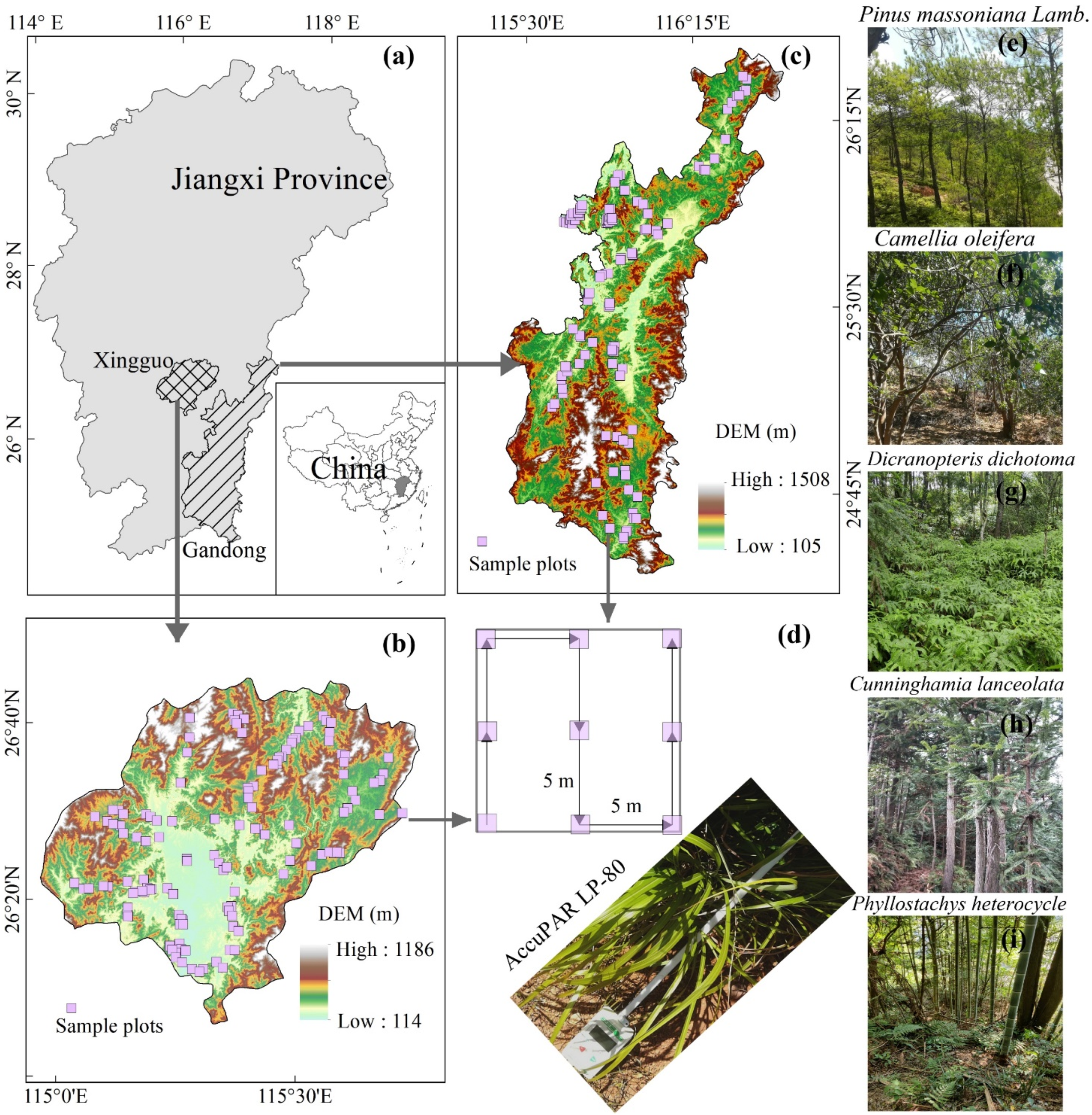
2.1. Study Areas

The two areas of Xingguo, 3211 km² (from 115°01′ E, 26°03′ N to 115°52′ E, 26°41′ N), and Gandong, 11,689 km² (from 115°09′ E, 25°32′ N to 116°38′ E, 26°36′ N), in the southern part of Jiangxi Province, China, were chosen for this study (Figure 1). These areas have similar forest types, land use patterns, topographies, and weather patterns. Both study areas include mountains, hills, and valleys, and are characterized by rugged and fragmented terrain with elevations ranging from 1055 to 1508 m. They have a medium subtropical monsoon climate with an average annual temperature ranging from 18.1 to 19.7 °C and an average annual precipitation of 1522.3 to 1919.6 mm [33], with frequent clouds, rain, and fog. Small areas of primary forest exist on the less accessible high mountains, but most of the existing forests are plantation and secondary forests [34]. The dominant plant species in the study areas are Pinus massoniana Lamb., Camellia oleifera, Dicranopteris dichotoma, Cunninghamia lanceolata, and Phyllostachys heterocycle.

2.2. Data

2.2.1. In Situ LAI Measurements

The field measurements of LAI of Xingguo and Gandong were collected from 23–29 November 2019, and 11–20 August 2020, respectively. Static values of field LAI were measured in the two study areas to examine the portability of the proposed ensemble strategy. Stratified random sampling was conducted within the forest landscape, topography, and physical accessibility of the areas, with the rule that the forest landscape should be homogeneous within each sample plot [23]. The types of forest landscape are defined according to the age of vegetation recovery and canopy structure [33,34]. Five types of forest landscapes are classified as (1). Tree-shrub-grass: forests consisting of tall trees (TSG), shrubs, and herbs; (2). Tree-grass: forests consisting mainly of trees and herbs (TG); (3). Shrub-grass: forests consisting mainly of shrubs and herbs (SG); (4). Non-wood product forest (NWP): forest producing fruit, edible oilseeds, etc.; (5). Bamboo forests (BB). Finally, 135 sample plots covering different forest landscape types were obtained in both Xingguo and Gandong (Figure 1b,c). The size of each square plot was approximately 10 m × 10 m, and their geographic locations were recorded based on their center coordinates using a handheld global positioning system (GPS) receiver. Field LAI measurements were measured at 0.2 m above the ground in each plot using a portable AccuPAR LP-80 photosynthetically active radiation meter [35]. For each plot, we performed three above-canopy observations in a nearby unshaded area to provide reference readings to minimize the impact of variation due to variation in incoming radiation. Nine below-canopy LAI observations were then collected and averaged to obtain an LAI value for the plot [11,35] (Figure 1d).

The LAI measured in the study areas varied from 0.36 to 10.85 m² m⁻², with means of 3.25 m² m⁻² in Xingguo and 4.32 m² m⁻² in Gandong (Figure 2a,b). NWP forests had the lowest LAI values, with mean values of 1.92 and 1.87 m² m⁻² in Xingguo and Gandong, respectively, while BL forests had the highest LAI values, with mean values of 5.24 and 3.92 m² m⁻² in Xingguo and Gandong, respectively.

2.2.2. Sentinel-1 Data and Preprocessing

SAR derivatives such as texture, patterns, and structural features provide unique opportunities for capturing physical properties of the forest scene can improve LAI mapping [14,15]. Two scenes of Sentinel-1B images covering Xingguo County and four scenes of Sentinel-1B images covering Gandong were downloaded from the Copernicus Open Access Center (https://scihub.copernicus.eu/, accessed on 1 November 2021). All of the downloaded data were acquired in IW (Interferometric Wide swath) mode in the GRDH (Ground Range Detected in High Resolution) processing (

Table 1. The Sentinel-1 and 2 imagery utilized in this study.

Study Area	Sensor	Remote Sensing Images	Product Type	Sensing Date	Season
Xingguo	Sentinel-1B	SAR	GRDH/IW	16 November 2019	Winter
				23 November 2019
	Sentinel-2B	MSI	S2MSI1C	06 December 2019
				13 December 2019
				06 December 2019
Gandong	Sentinel-1B	SAR	GRDH/IW	15 July 2020	Summer
				21 July 2020
	Sentinel-2B	MSI	S2MSI1C	13 July 2020
				19 August 2020
				30 July 2020
				30 July 2020

). For each SAR image scene, speckle filtering, radiometric calibration, terrain correction, and geocoding were performed using SNAP (version 6.0, European Space Agency) [36,37]. The backscatter intensities of VV (horizontal transmit-horizontal channel) and VH (horizontal transmit-vertical channel bands) were then generated based on mean values for 3 × 3 pixel windows.

Texture measures derived from the SAR band have great potential in vegetation monitoring because they can provide information on the structure and physical properties of the land surface [38]. We obtained the texture feature using the Grey Level Co-occurrence Matrix (GLCM) [39], which is defined by the joint probability density of pixels in two positions; it reflects both the distribution of the brightness and the distribution of pixels with identical or similar brightness [38]. A set of texture feature indices were extracted from the final VV and VH bands, including correlation texture, contrast texture, homogeneity texture, dissimilarity texture, variance texture, entropy texture, energy texture, and mean texture [38,39] (

Table 2. Remote sensing indices from ALOS-1DEM, Sentinel-1 SAR, and Sentinel-2 MSI for forest LAI mapping.

Sensor	Types	Indices	Definition
Sentinel-1	Backscatter	VH	Normalized backscatter coefficient of VH channel (dB)
		VV	Normalized backscatter coefficient of VV channel (dB)
		V/H	VV/VH
		VV_CON	Contrast, measure the statistics derived from the GLCM
	Texture	VV_DIS	Dissimilarity
		VV_IDM	Inverse difference moment
		VV_ASM	Angular second moment
		VV_ ENT	Entropy
		VV_AVG	Mean
		VV_COR	Correlation
		VH_CON	Same with above-mentioned texture
		VH_DIS
		VH_IDM
		VH_ASM
		VH_ ENT
		VH_AVG
		VH_COR
		ARVI	Atmospherically resistant vegetation index, (B8 − B5 − y(B5 − B1))/(B8 + B5 − y(B5 − B1))
Sentinel-2	Vegetation indices	CI	Coloration Index, (B4 − B2)/B4
		DVI	Difference vegetation index, B8 − B4
		NDVI	Normalized difference vegetation index, (B8 − B4)/(B8 + B4)
		GNDVI	Green normalized difference vegetation index, (B8a − B3)/(B8a + B3)
		IPVI	Infrared percentage vegetation index, B8/2(B8 + B4) × (NDVI + 1)
		IRECI	Inverted red-edge chlorophyll index, (B7 − B4)/(B5/B6)
		MSAVI	Modified soil-adjusted vegetation index, B8 + 0.5 − [(2B8 + 1)2 − 8(B8 − B5)]0.5
		MSAVI2	Modified soil-adjusted vegetation index 2, B8 + 0.5 − [(2B8 + 1)2 − 8(B8 − B4)]0.5
		PVI	Perpendicular vegetation index, 1/(α0.5 + 1) × (B8a – αr − β)
		SAVI	Soil adjusted vegetation index, (B8 − B4)/(B8 + B5 + L) × (1 + L)
		TNDVI	Transformed NDVI, [(B8a − B4)/(B8a + B4) + 0.5]0.5
		WDVI	Weighted difference vegetation index, B8a − αB5, α = nir soil/red soil
		RVI	Simple ratio vegetation index, B8/B4
		RI	Normalized difference red/green redness index, (B4 − B3)/(B4 + B3)
		MTCI	Meris terrestrial chlorophyll index, (B6 − B5)/(B5 − B4)
		REIP	REIP Red-edge infection point index, 700 + 40 × [(B4 + B7)/2− B5]/(B6−B5)
		NDVI2	Normalized difference vegetation index 2, (B12 − B8)/(B12 + B8)
		RDVI	Renormalized difference vegetation index, (B8 − B4)/[(B8 + B4)0.5]
		MSBI	Misra soil brightness index, 0.406B3 + 0.600B4 + 0.645B6 + 0.643B8a
ALOS-1 DEM	Topographical parameters	TWI	Topographic wetness index
		ELE	Elevation
		SLO	Slope
		ASP	Aspect
		PRC	Profile curvature
		PLC	Plan curvature
		RLS	Relief of land surface
		TWI	Topographic wetness index
		SPI	Stream power index
		SL	Slope length, a factor calculated by Universal Soil Loss Equation
		TRI	Terrain ruggedness index

).

2.2.3. Sentinel-2 Data and Preprocessing

The Sentinel-2 mission carries two Multi Spectral Instruments (MSIs) that samples 13 bands at three spatial resolutions (10, 20, and 60 m), providing wide-swath multispectral images [13,20]. The Level 2A (Bottom Of Atmosphere) Sentinel-2B reflection images covering Xingguo and Gandong were collected from the Copernicus Sentinel Scientific Data Hub (Table 1). The MSI data employed in this study were those with the least cloud cover and the imaging time closest to the time of ground LAI measurement over the LAI plots. For all MSI images, the 20 and 60 m bands were resampled to a resolution of 10 m using the cubic method on the SNAP platform [40]. Then, 20 commonly used spectral indices (Table 2) were extracted from each reflectance image of the study area.

2.2.4. ALOS-1 DEM Data

The Panchromatic Remote Sensing Stereo Mapping Instrument was an active microwave sensor using the L-band for global elevation mapping onboard the ALOS launched by JAXA, which operated from 2006 to 2011 [41]. The ALOS-1 DEM product was proven to provide highly accurate information on land surface topography [42]. ALOS DEM data for the study area with a spatial resolution of 12.5 m was collected from the Alaska Satellite Facility (https://search.asf.alaska.edu/, accessed on 1 November 2021). The downloaded DEM data were processed by image stitching and cropped to cover only the study area, then 11 terrain attributes were extracted using SAGAGIS (http://www.saga-gis.org/en/index.html, accessed on 1 November 2021). All DEM-derived variables were registered in Universal Transverse Mercator (UTM) Zone 50 N based on the WGS-84 coordinate system and resampled to a spatial resolution of 10 m for compatibility with the pre-processed Sentinel-1 and 2 series.

2.3. Variable Selection and Variables Importance

A total of 62 variables were extracted in this work (Table 2). Collinearity among predictors could increase the uncertainty of predictive models; therefore, variable selection was necessary. Variables with a non-significant association with LAI (p > 0.05) and strongly correlated variables of the same type (r < 0.8) were, therefore, removed [17,43].

The importance of each variable in mapping forest LAI was investigated using permutation feature importance (PFI). PFI is a random forest-based measurement tool for interpreting the relevance of features of interest to the performance of machine learning models [44]. Briefly, it generates random noise to replace a feature, with the random noise values being generated by shifting the values of the original predictors [45]. RF regression is then performed to measure the average loss in model accuracy (root mean square error, RMSE) as each feature is shuffled, yielding the importance of each variable. The PFI analysis was performed using the iml package of the R statistical computing environment.

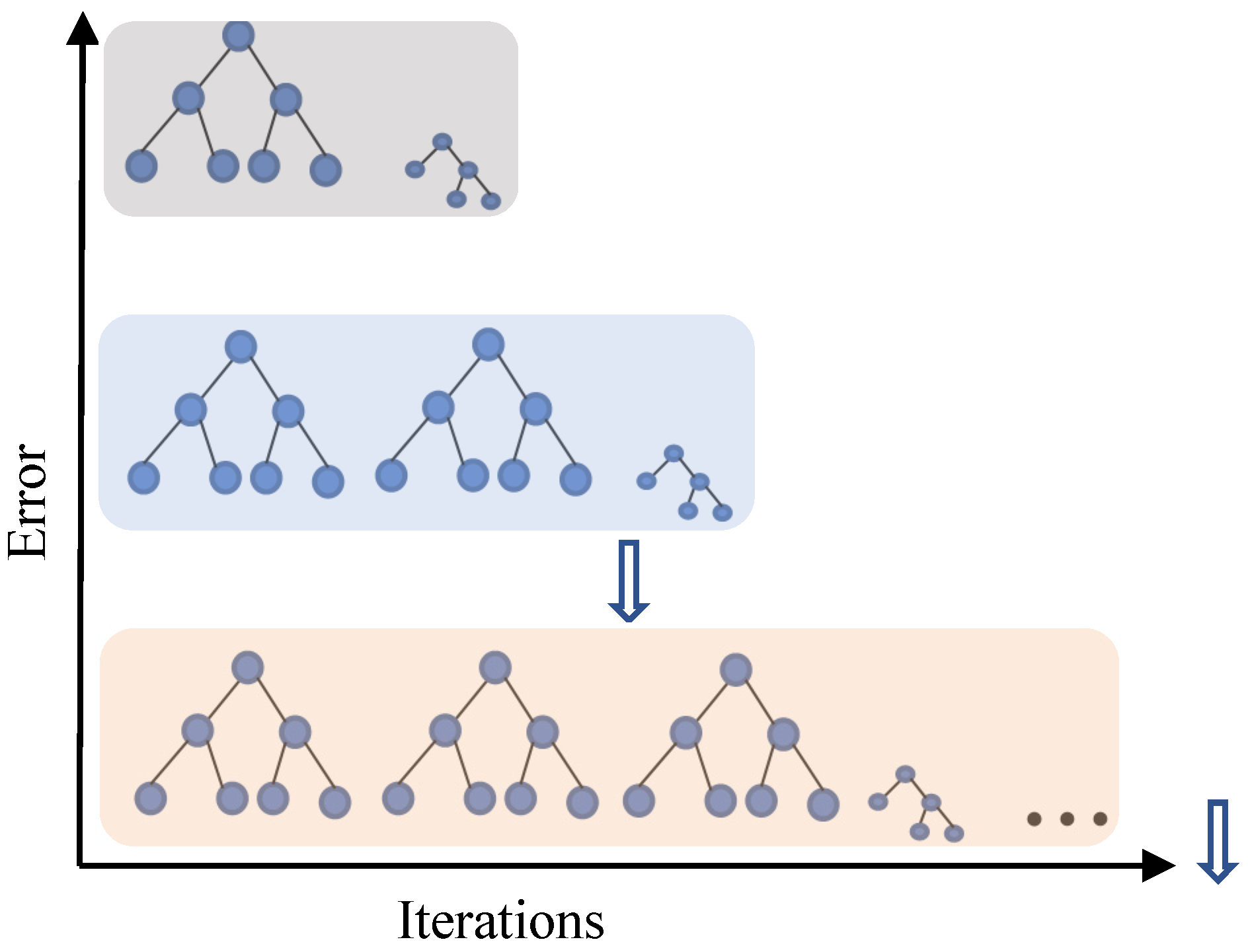
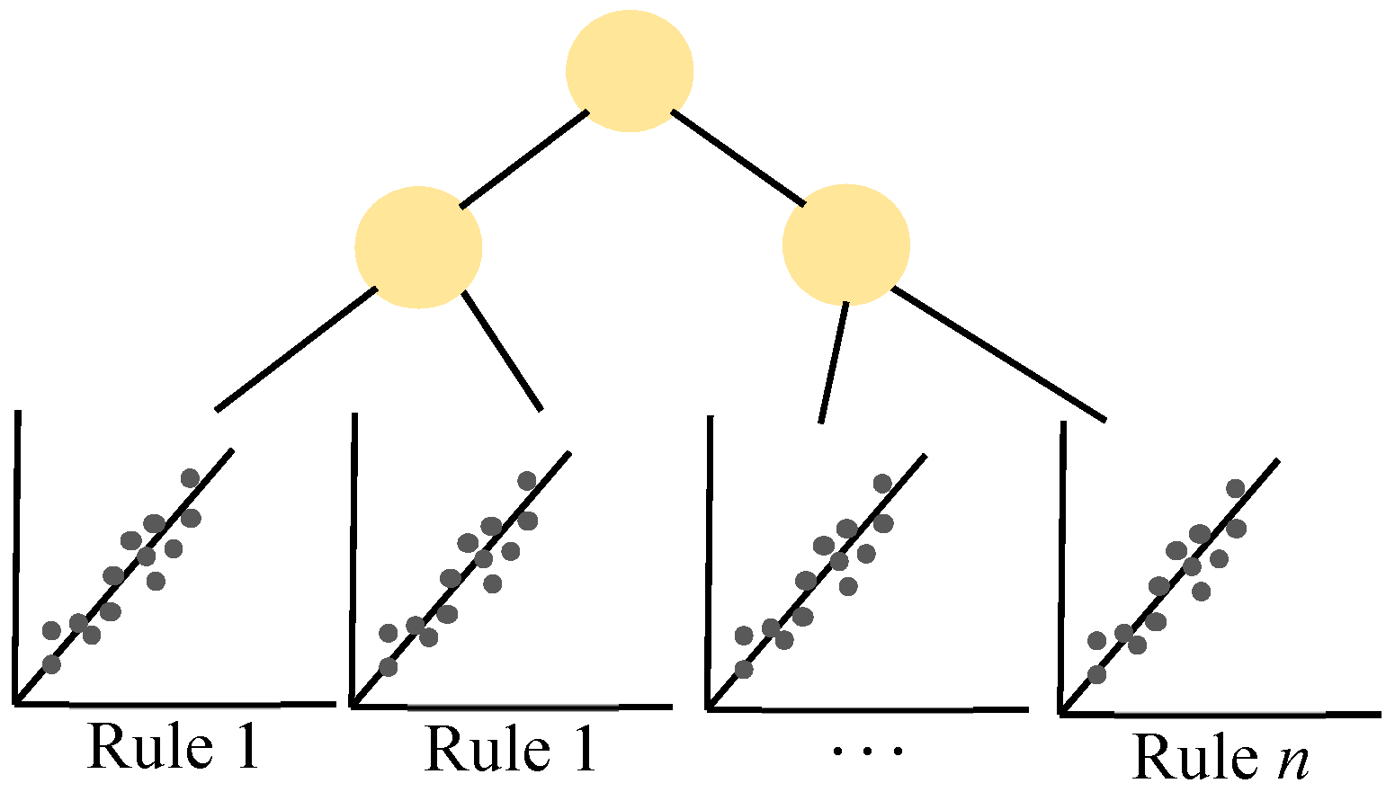
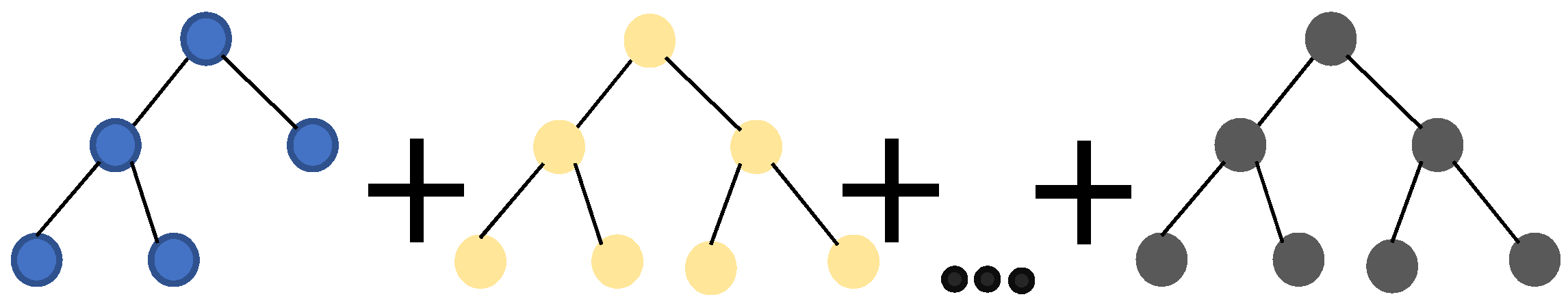
2.4. Stacking Learning

SL is a hierarchical learning method with a lower level comprising a set of base learners and a higher level of meta-learners [46]. It differs from conventional ML methods in that it is not a specific algorithm but a free ensemble scheme that allows the merging of multiple base learners into a new model via a stacking rule; both the stacking rule and the set of base learners may be chosen freely [31]. Typically, a meta-feature dataset is created using a set of base learners at level 0 that generate initial predictions from raw data using various ML algorithms. The meta-learner at level 1 then functions as a generalizer, making final predictions of the response and correcting for biases in the new input features through aggregation. A diverse set of level 0 base learners, including SVM, ANN, GPR, Cubist, KNN, Classification and Regression Trees (CART), AdaBoost Classification Trees (ABCT), Extreme Learning Machine (ELM), Boosted Regression Tree (BRT), and EXtreme Gradient Boosting machines (XGBoost), were used to generate the basic regressions used to build new input features for the SL model. RF was then used at level 1 to produce the final forest LAI estimate. As high-dimensional statistical methods, these models are capable of handling complex nonlinear relationships, as illustrated in Figure A1, Figure A2, Figure A3, Figure A4, Figure A5, Figure A6, Figure A7, Figure A8, Figure A9, Figure A10 and Figure A11 andbriefly described in Appendix A.

2.5. Forest LAI Mapping

As the field LAI sampling intervals and the spatial resolution of the processed remote sensing variables were found to be consistent at a scale of 10 m, we built SL models at the 10-meter scale using multi-source satellite images to map the spatial patterns of forest LAI across the study areas. Forest LAI modeling was performed using the machine learning library of the R programming platform according to the workflow shown in Figure 3.

2.5.1. Tuning the Hyperparameters for the Stacking Learning Models

Hyperparameters are used to configure ML models. Before evaluating and comparing the learners, the hyperparameters of each algorithm were optimized using a grid search method with 10-fold cross validation [47]. The key tuning parameters and their possible ranges for each learner are shown in

Table 3. Hyperparameters tuned and their configurations for each algorithm.

Algorithm	R Package	Hyperparameters Tuned	Range
CART	rpart	cp, the complexity parameter.	0.048
Cubist	cubist	committees, the number of committee models.	1–100
		neighbors, the number of neighbors used to correct the model predictions.	0–10
BRT	GBM	n.trees, the number of trees to fit.	50–1000
		interaction.depth, the number of splits in each tree.	1–20
		shrinkage, the rate at which the model descends along the gradient.	0.01–1
		n.minobsinnode, the minimum number of observations of the terminal node of the tree.	1–50
RF	randomForest	ntree, the number of trees to grow into a forest.	50–1000
		mtry, the number of variables to be considered at each split.	1–30
XGBoost	xgboost	nrounds, the maximum number of iterations.	1–1000
		max_depth, the depth of the tree.	1–10
		eta, the learning rate.	0.01–0.5
		gamma, prevents overfitting.	0–1
		colsample_bytree, the number of variables supplied to a tree.	0.1–1
		min_child_weight, the minimum number of instances required in a child node.	0–3
ANN	nnet	size, the number of units in the hidden layer.	1–10
		decay, parameter for weight decay.	0.001–0.05
KNN	caret	k, number of neighbors considered.	1–20
SVM	e1071	sigma, scaling parameters of the hypothetical Laplace distribution.	0.01–0.5
		C, the regularization term in the Lagrange formulation	1–10
GPR	kernlab	degree, parameter for the Polynomial kernel “polydot”.	1–10
		scale, parameter for the Polynomial kernel “polydot”.	0.001–0.5
ELM	elmNN	nhid, number of hidden Units, numeric.Activation Function (actfun, character)	1–100
		actfun, activation function.	linear
ABCT	adaboost	mstop, number of boosting iterations.	50–1000
		AIC prune.	yes

. It is also essential to determine the number of base learners (NBL) in the SL model that give the optimal structure, because the structure of the SL model influences the precision and training time. To explore the sensitivity of the SL model’s performance to the NBL, several experiments were conducted to measure prediction accuracy using different ML ensembles. Whenever the number of base learners was changed, the worst-performing base learner was removed and the others were reserved for stacking; for example, when the NBL was set to 2, the first two regressors were selected as base learners.

2.5.2. Model Accuracy Assessment

To evaluate the capabilities of SL approaches and compare the performance of SAR, MSI, and DEM data (and their combinations) for forest LAI estimation, six groups of variables were used as regression model inputs. First, six groups of predictor variables derived from the Sentinel-1 (SAR), Sentinel-2 (MSI), and ALOS DEM (DEM) datasets were defined as follows: SAR, DEM, MSI, MSI + SAR, MSI + DEM, and MSI + SAR + DEM. LAI estimation models based on each variable group were then trained and evaluated using a ten-fold cross-validation approach [48]. In ten-fold cross-validation, the measured data sets are randomly split into 10 equally or similarly sized segments, of which 9 are combined and used as a training set, while the tenth is used as the testing set. This process is repeated ten times, with a different segment being used as the testing set on each occasion. Additionally, the train-test splits are the same for each regression model. The accuracy of the models’ predictions was evaluated by computing statistical measures based on the difference between the measured and predicted LAI, namely, the coefficient of determination (R²), mean error (ME), and root mean squared error (RMSE), calculated using Equations (1)–(3), respectively.

$$R^2=1-\frac{{\displaystyle {\sum }_{i=1}^n{\left(y_i-{\widehat{y}}_i\right)}^2}}{{\displaystyle {\sum }_{i=1}^n{\left(y_i-\overline{y}\right)}^2}}$$

(1)

$$MAE={\displaystyle \sum _{i=1}^n\frac{\left|y_i-{\widehat{y}}_i\right|}{n}}$$

(2)

$$RMSE=\sqrt{{\displaystyle \sum _{i=1}^n\frac{{\left(y_i-{\widehat{y}}_i\right)}^2}{n}}}$$

(3)

Here, $\widehat{y}$ is the estimated LAI value obtained using the model, y_i is the corresponding observed LAI value, $\overline{y}$ is the mean observed LAI, and n is the number of samples used for validation. Multiple data sources and SL techniques were used to create LAI products with a spatial resolution of 10 m to capture the fine spatial heterogeneity of subtropical forests.

3. Results

3.1. Correlation Analysis and Variable Selection

On the basis of Pearson correlation analysis, 23 variables were selected to estimate the forest LAI in Xingguo and Gandong, respectively (

Table 4. Correlation coefficients for the measured LAI and selected variables derived from the ALOS-1 and Sentinel-1 and 2 datasets. ** and * indicate cases with p values below 0.01 and 0.05, respectively.

Group	Types	Variable	Xingguo	Gandong
ALOS-1	Topographic parameters	LS	0.27 *	0.44 **
		SLO	0.28 *	0.46 **
		ELE	0.36 **	0.47 **
		TWI	−0.30 **	−0.32 **
Sentinel-1	Backscatter	VH	0.24 *	0.20 *
	Texture	VH_cor	0.30 *	0.24 *
		VH_Mean	0.29 **	0.19 *
		VV_Ene	0.33 **	0.20 *
		VV_Max	0.27 **	0.19 *
Sentinel-2	Soil indices	RI	−0.43 **	−0.30 *
		CI	−0.72 **	−0.58 **
	Vegetation indices	ARVI	0.61 **	0.73 **
		DVI	0.36 **	0.43 **
		GNDVI	0.62 **	0.66 **
		IPVI	0.54 **	0.71 **
		IRECI	0.29 *	0.72 **
		MSAVI	0.26 *	0.53 **
		MSAVI2	0.28 *	0.55 **
		NDVI	0.79 **	0.70 **
		PVI	0.56 **	0.43 **
		SAVI	0.27 *	0.56 **
		TNDVI	0.55 **	0.68 **
		WDVI	0.25 *	0.52 **

). Of the topographic variables, LS, SLO, ELE, and TWI were significantly correlated with the LAI at the 0.01 level and above. Of the SAR-derived variables, texture features correlated more strongly with the LAI than the backscattered intensity from the C-band of the VH. The LAI was significantly and positively correlated with VH_Cor and VH_Mean. The LAI during winter (Xingguo) was sensitive to the backscattering coefficient of the VH, VV_Asm, and VH_Var, while the LAI during summer (Gandong) was more sensitive to VV_Ene and VV_Max. This indicates that the variation in the backscattering intensity and phase difference explain the effect of seasonal variation on the LAI. Among the vegetation spectral indices, NDVI, GNDVI, and ARVI had the highest correlation with the LAI in Xingguo during winter, while ARVI, IRECI, IPVI, and NDVI showed the strongest correlation with the LAI in Gandong during the summer. The vegetation indices showed stronger correlations than the soil indices. Additionally, the r values for the DEM- and SAR-derived variables were lower than those for the MSI variables.

3.2. Evaluation and Comparison of Different Models and Datasets

Figure 4 shows how the performance of the SL models (evaluated in terms of the R², RMSE, and MAE) varied with the NBL; the average model accuracy initially increased with the NBL but then stabilized. The best predictive performance for the LAI in Xingguo was obtained using SL models taking the DEM, SAR, MSI, SAR + MSI, DEM + MSI, and DEM + SAR + MSI predictor variable groups as inputs with NBL values of 10, 10, 8, 8, 7, and 7, respectively. The best predictions of the LAI in Gandong were obtained with the same groups using NBL values of 8, 8, 8, 7, 7, and 7, respectively.

For the inputs of the DEM, SAR, MSI, DEM + MSI, SAR + MSI, and DEM + SAR + MSI variables, the validation indices of SL models predicting the LAI in Xingguo: the R² improved by 173%, 335%, 24%, 23%, 23%, and 21%, respectively; the MAE decreased by 51%, 49%, 66%, 67%, 66%, and 71%, respectively; and the RMSE decreased by 44%, 40%, 61%, 62%, 59%, and 64%, on average, respectively, compared to individual ML models (

Table 5. The accuracies of accuracy comparison of the different machine learning models in Xingguo and Gandong.

Inputs	Model	Xingguo			Gandong
		R2	MAE	RMSE	R2	MAE	RMSE
DEM	ANN	0.27	1.15	1.40	0.13	1.87	2.34
	KNN	0.20	1.15	1.39	0.11	1.89	2.29
	SVM	0.18	1.19	1.47	0.16	1.76	2.27
	GPR	0.31	1.15	1.39	0.17	1.81	2.24
	CART	0.28	1.23	1.52	0.11	1.92	2.37
	BRT	0.30	1.12	1.36	0.14	1.97	2.44
	Cubist	0.30	1.12	1.37	0.15	1.84	2.31
	XGBoost	0.29	1.27	1.54	0.15	2.18	2.40
	ABCT	0.32	1.08	1.32	0.17	1.85	2.22
	ELM	0.28	1.11	1.34	0.13	1.86	2.30
	SL	0.72	0.56	0.79	0.57	1.12	1.54
Sentinel-1 (SAR)	ANN	0.11	1.19	1.51	0.08	2.06	2.58
	KNN	0.11	1.17	1.46	0.08	1.88	2.32
	SVM	0.12	1.18	1.48	0.11	1.94	2.41
	GPR	0.20	1.17	1.44	0.15	1.84	2.26
	CART	0.13	1.24	1.56	0.11	2.01	2.45
	BRT	0.19	1.12	1.43	0.10	1.95	2.41
	Cubist	0.18	1.17	1.45	0.12	2.05	2.47
	XGBoost	0.17	1.32	1.64	0.09	2.04	2.29
	ABCT	0.21	1.11	1.40	0.14	1.89	2.29
	ELM	0.19	1.17	1.46	0.11	2.01	2.45
	SL	0.66	0.60	0.89	0.62	1.07	1.46
Sentinel-2 (MSI)	ANN	0.81	0.74	0.76	0.81	0.93	1.26
	KNN	0.72	0.66	0.84	0.71	1.25	1.33
	SVM	0.73	0.72	1.01	0.74	1.10	1.37
	GPR	0.77	0.89	1.25	0.76	1.15	1.27
	CART	0.64	1.01	1.28	0.75	1.15	1.41
	BRT	0.81	0.61	0.70	0.81	0.89	1.14
	Cubist	0.80	0.59	0.81	0.82	0.87	1.11
	XGBoost	0.79	0.64	0.77	0.81	1.01	1.27
	ABCT	0.82	0.58	0.78	0.84	0.79	1.03
	ELM	0.80	0.61	0.79	0.82	0.97	1.29
	SL	0.95	0.23	0.34	0.95	0.34	0.51
DEM + MSI	ANN	0.82	0.49	0.67	0.82	0.89	1.20
	KNN	0.73	0.64	0.84	0.73	1.01	1.30
	SVM	0.75	0.67	0.92	0.76	1.08	1.25
	GPR	0.79	0.86	1.09	0.80	1.14	1.18
	CART	0.67	0.98	1.26	0.75	1.26	1.38
	BRT	0.81	0.53	0.68	0.82	0.86	1.12
	Cubist	0.81	0.58	0.76	0.82	0.83	1.10
	XGBoost	0.80	0.59	0.76	0.82	0.99	1.19
	ABCT	0.83	0.48	0.65	0.84	0.78	1.02
	ELM	0.82	0.51	0.67	0.84	0.90	1.20
	SL	0.96	0.20	0.30	0.95	0.33	0.50
SAR + MSI	ANN	0.81	0.58	0.67	0.81	0.92	1.23
	KNN	0.73	0.65	0.84	0.72	1.09	1.31
	SVM	0.74	0.68	0.92	0.74	1.08	1.34
	GPR	0.78	0.87	1.14	0.80	1.14	1.18
	CART	0.66	1.00	1.26	0.75	1.53	1.39
	BRT	0.81	0.54	0.69	0.82	0.87	1.13
	Cubist	0.80	0.59	0.80	0.82	0.86	1.11
	XGBoost	0.80	0.59	0.77	0.81	1.01	1.24
	ABCT	0.82	0.48	0.65	0.84	0.79	1.03
	ELM	0.81	0.52	0.67	0.82	0.92	1.23
	SL	0.95	0.21	0.33	0.94	0.33	0.52
DEM + SAR + MSI	ANN	0.83	0.48	0.67	0.82	0.88	1.18
	KNN	0.75	0.62	0.81	0.79	0.97	1.27
	SVM	0.77	0.65	0.91	0.76	1.03	1.14
	GPR	0.81	0.84	1.08	0.82	1.05	1.18
	CART	0.69	0.98	1.24	0.75	1.26	1.29
	BRT	0.82	0.52	0.67	0.82	0.85	1.11
	Cubist	0.81	0.54	0.73	0.83	0.83	1.09
	XGBoost	0.81	0.59	0.75	0.82	0.95	1.13
	ABCT	0.83	0.47	0.64	0.84	0.78	1.01
	ELM	0.84	0.51	0.65	0.83	0.86	1.15
	SL	0.96	0.17	0.28	0.96	0.30	0.47

). Similarly, the validation indices of the SL model for predicting the LAI in Gandong: the R² improved by 311%, 492%, 21%, and 19%, respectively; the MAE decreased by 41%, 46%, 66%, 65%, 67%, and 68%; and the RMSE decreased by 34%, 39%, 59%, 58%, 57%, and 59%, on average, respectively. Overall, the SL models achieved higher prediction accuracy than the ten individual ML models. This indicates that the SL model fits better than the individual ML model regardless of the input variables, and therefore, SL has good prospects for retrieving the forest LAI.

Among the three types of predictor variables, the MSI derivatives obtained a higher prediction accuracy than the SAR and DEM data. For example, when predicting the LAI in Xingguo, the validation indices for the MSI variables were as follows: the R², the MAE, and the RMSE in the range of 0.64 to 0.95, 0.23 to 1.01, and 0.34 to 1.28, respectively, while those for the DEM variables were as follows: the R², the MAE, and the RMSE in the range of 0.20 to 0.72, 0.56 to 1.27, and 0.79 to 1.52, respectively, and those for the SAR variables were as follows: the R², the MAE and the RMSE in the range of 0.11 to 0.66, 0.60 to 1.32, and 0.89 to 1.64, respectively. For the LAI estimation, overall, the DEM data yielded better predictions than SAR.

For all the models, the incorporation of the SAR and MSI data improved the prediction accuracy (Table 5). There are overestimations and underestimations found for some of the sample plots for the single-source models both in Xingguo and Gandong (Figure 5 and Figure 6). Given the same model, compared with those from the inputs of single-source data, the lower uncertainty was obtained by using the dual- or triple-source data. Specifically, the addition of the SAR variables using the SL model compared to the use of only the MSI data reduced the MAE and RMSE by 9% and 3%, respectively, in Xingguo and by 3% and 2%, respectively, in Gandong. Similarly, with the addition of the DEM variables, the MAE and RMSE of the SL model were reduced by 13% and 12%, respectively, in Xingguo, and by 3% and 2%, respectively, in Xingguo. The highest prediction accuracy was achieved when the DEM, SAR, and MSI images were applied together. Correspondingly, the MAE and RMSE of the SL model based on triple-source data were reduced by 26 and 18%, respectively, in Xingguo, and by 12% and 8%, respectively, in Gandong. These improvements were also verified using individual ML models.

3.3. Variable Importance

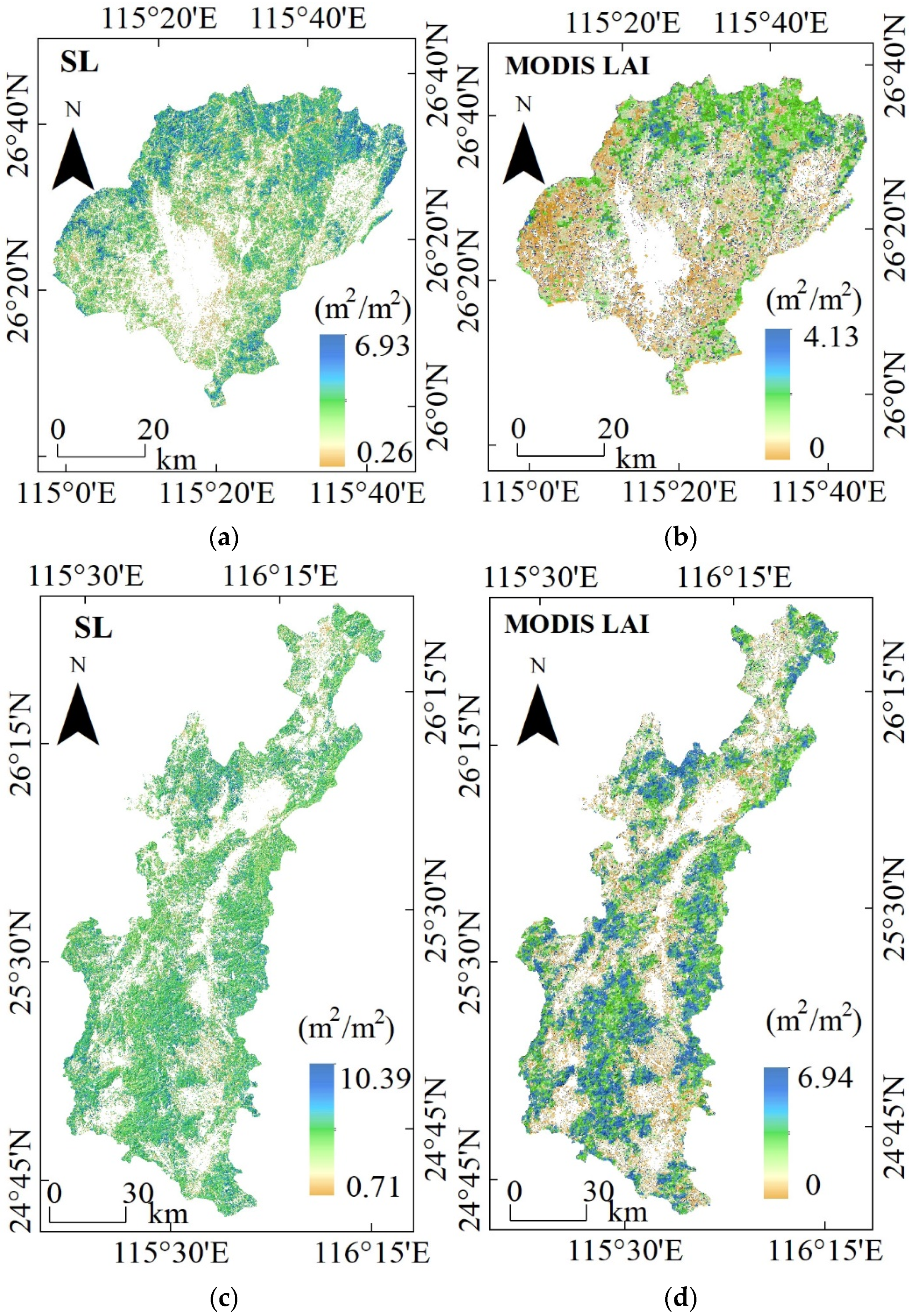
The relative importance of each variable obtained from the PFI algorithm is shown in Figure 7. The top three most important variables influencing the variation of the LAI in both Xingguo and Gandong were the MSI variables, indicating that optical imagery was the most important contributor to predicting the LAI. For the LAI variation in Xingguo during the winter, the MSI variables (65.61% relative importance) were the most important explanatory variables, followed by the topographic variables (18.48%). The MSI and DEM variables explained 68.67 and 16.21% of the LAI variation in Gandong during summer, respectively. While the SAR variables were ranked in the bottom five in terms of importance, they explained 15.91 and 15.12% of the spatial variation of the LAI in Xingguo and Gandong, respectively. Moreover, the contributions of the DEM and SAR variables to the LAI variations during winter are higher than those to the LAI variations during summer.

3.4. LAI Maps

The LAI maps were generated using the average of 100 runs of the SL model based on the combination of all the predictors. Additionally, the standard deviation (SD) was calculated to assess the prediction uncertainty. A strong LAI spatial variation can be observed in Figure 8. The highest LAI predictions were found in the northern part of Xingguo and the southern part of Gandong. These parts of the study areas were mainly native forests, displaying higher elevation and with a lower erosion susceptibility, which favors forest growth and explains the high LAI. For the predicted LAI in Xingguo, the mean and SD were 3.02 and 0.06 m²/m², respectively, and for the predicted LAI in Gandong, the mean and SD were 4.05 and 0.08 m²/m², respectively. The low value of SD for the 100th predicted LAI indicates that the SL models using a combination of the SAR, DEM, and MSI variables have stable prediction capabilities. The maps of the predicted LAI had a similar spatial pattern to the MODIS LAI (MYD15A2H, with a resolution of 500 m) product (Figure A12 in Appendix B), indicating that the LAI predictions presented in this study are reliable.

4. Discussion

4.1. Roles of Sentinel-1 and 2 and ALOS-DEM in Forest LAI Estimation

Correlation coefficients (Table 3), variable importance calculations (Figure 7), and measures of predictive model performance were used to evaluate the contributions of the MSI, SAR, and DEM data to the LAI estimation (Table 4, Figure 5 and Figure 6). In accordance with previous studies, the MSI was more useful than the SAR and DEM for the LAI estimation, providing a wider range of the predicted LAI values. This is likely because the MSI data consist of optical sensor readings; spectral indices from the narrow-band, red-edge, and SWIR spectral regions are sensitive to green vegetation and are useful for retrieving forest phenology, physiology, and structure [13,23,28]. However, the MSI suffers from data saturation due to the forest canopy’s shading of solar radiation in thick forest zones, which causes the MSI to a record horizontal vegetation structure more effectively than vertical biophysical characteristics [49]. As a result, there is limited heterogeneity in the spectral index data for stands with high LAIs (LAI > 7) [49,50] such as those of the studied forests, which have complex structures with a multistoried canopy architecture and high vegetation cover [16].

SAR variables provide the poorest predictive performance. This was primarily attributed to saturation of the SAR-derived backscatter coefficients [17]. Volume scattering is usually the dominant source of plant backscatter, and the tree canopy contributes the most volume scattering [14,51]. Therefore, as forest cover increases, the sensitivity of the SAR signal to understory forests and soil is significantly reduced. The observed LAI values in the study region are generally above three, which is likely to represent the saturation threshold for the C-band SAR backscatter [52]. The low saturation value for the C-band SAR data is due to the long wavelength and long pulse duration of the C-band, which results in high contamination by speckle noise [17]. This suggests that the SAR-derived texture characteristics are more useful than the backscatter coefficient for forecasting the forest LAI [17,53].

The DEM variables outperformed the SAR variable for the LAI prediction because the topography is more relevant to the LAI in the studied area than the SAR variables (Table 3). Forest structure parameters could be quantitatively modeled by topographic derivatives, and therefore, there could be significant relationships between the DEM variables and the forest LAI [54]. The most important DEM variables for large-scale mapping the spatial variability of the LAI in subtropical forests were found to be Slope, ELE, TWI, and LS. ELE and Slope can reflect the accessibility of human interference and the development of microclimates, which, in turn, affect the distribution of forest communities [18,34]. TWI is a sensitive indicator of soil water content, and can also slow down organic matter decomposition and, thus promote vegetation growth [33,34]. LS can capture soil erosion risk at different landscape positions where overland flow and slope dominate the soil scouring processes and is correlated with the distribution of forest and the LAI [18,33]. The study areas are distinguished by a high proportion of mountains and hills, as well as relatively large topographic variations. To some extent, topography controls soil fertility variations and geological hazard susceptibility as a constraint on forest distribution and the LAI variations [54].

Thus, this study demonstrated that using multi-sensor data for the LAI prediction yields better predictive performance than using optical data alone and also reduces the uncertainty of the predictive model.

4.2. Usefulness of Stacking Learning Models for Forest LAI Quantification

As a novel ML technique, SL is particularly flexible in incorporating the different strengths of individual ML models. This study revealed its general superiority in estimating the forest LAI using multiple input variables under different climate regimes. The high predictive performance of the SL methods was attributed to the diversity of base learners that were used and the choice of effective incorporation rules [31]. As noted by Schwenker [26], training data alone cannot provide sufficient information to identify a single best learner, necessitating the stacking of several base learners. A varied set of base learners provides a greater opportunity to correct for biases arising from individual models and reduces the dependence on sample size [24,26].

We also found that the NBL significantly affected the SL model performance. However, many previous prediction studies [25,27,28,29,30] did not attempt to optimize the NBL when generating SL models. In this work, the best NBL for estimating the LAI was determined through a comparative analysis of SL models (Figure 4), which revealed that the use of too many or too few base learners reduced the accuracy of SL models. Indeed, the greater the NBL is, the greater the chance is of the overfitting of the SL model [26,55]. This suggests that picking an appropriate number and type of base learner is preferable to randomly selecting base learners for the construction of accurate SL models.

The improved accuracy of the SL technique allows the use of low-correlation variables as separate functions for model fitting [24,26]. Therefore, spectral and grayscale data for individual pixels can be combined with information on heterogeneity and coerced to fit more reliable nonlinear relationship models for the forest LAI estimation based on either individual indices or raw bands. This allows another important goal of using low-correlation variables to be achieved, namely, mining more valuable knowledge to enhance model accuracy (Figure 5a,b and Figure 6a,b). In addition, the performance of the SL model is also affected by the meta learner that is used to fit the base learners. Therefore, we recommend using specific experimental data to calibrate and select the optimal meta learner to improve the accuracy of the LAI estimation.

5. Conclusions

This work investigated the potential of integrating multi-sensor imagery from the Sentinel-1, Sentinel-2, and ALOS-1 DEM using the SL machine learning algorithm, for retrieving the forest LAI in the subtropical forests of southern China. The evaluations using field LAI measurements showed that the proposed framework offered an encouraging performance. It was found that combining the DEM and SAR data with the MSI images improves the accuracy while reducing the uncertainty when compared to analyses based on only optical data. The spectral indices from the MSI images were the key variables for capturing the spatial variability of the forest LAI. Topographic parameters from the DEM are more important than the C-band SAR back scatterers and their texture features. The SL algorithm can be considered as one of the most adaptable ML algorithms for further research on the LAI estimation. Not only were the relationships between the LAI observations and environmental covariates quantified by various individual ML models preserved based on the meta-learner, but the algorithm greatly improved the prediction performance when used as a regression method. The proposed combined strategy of multi-model, multi-source remote sensing data reduces this structural uncertainty and therefore provides greater robustness and reliability than individual models and single-source data in retrieving and mapping the forest LAI.

References

1. Zhou, G.; Houlton, B.Z.; Wang, W.; Huang, W.; Xiao, Y.; Zhang, Q.; Liu, S.; Cao, M.; Wang, X.; Wang, S. Substantial reorganization of China’s tropical and subtropical forests: Based on the permanent plots. Glob. Change Biol. 2014, 20, 240–250. [Google Scholar] [CrossRef] [PubMed]
2. Harris, N.L.; Gibbs, D.A.; Baccini, A.; Birdsey, R.A.; De Bruin, S.; Farina, M.; Fatoyinbo, L.; Hansen, M.C.; Herold, M.; Houghton, R.A. Global maps of twenty-first century forest carbon fluxes. Nat. Clim. Change 2021, 11, 234–240. [Google Scholar] [CrossRef]
3. Mori, A.S.; Dee, L.E.; Gonzalez, A.; Ohashi, H.; Cowles, J.; Wright, A.J.; Loreau, M.; Hautier, Y.; Newbold, T.; Reich, P.B. Biodiversity-productivity relationships are key to nature-based climate solutions. Nat. Clim. Change 2021, 11, 543–550. [Google Scholar] [CrossRef]
4. Wenhua, L. Degradation and restoration of forest ecosystems in China. For. Ecol. Manag. 2004, 201, 33–41. [Google Scholar] [CrossRef]
5. Chen, Y.; Wang, K.; Lin, Y.; Shi, W.; Song, Y.; He, X. Balancing green and grain trade. Nat. Geosci. 2015, 8, 739–741. [Google Scholar] [CrossRef]
6. Tong, X.; Brandt, M.; Yue, Y.; Ciais, P.; Jepsen, M.R.; Penuelas, J.; Wigneron, J.-P.; Xiao, X.; Song, X.-P.; Horion, S. Forest management in southern China generates short term extensive carbon sequestration. Nat. Commun. 2020, 11, 129. [Google Scholar] [CrossRef]
7. Soudani, K.; François, C.; Le Maire, G.; Le Dantec, V.; Dufrêne, E. Comparative analysis of IKONOS, SPOT, and ETM+ data for leaf area index estimation in temperate coniferous and deciduous forest stands. Remote Sens. Environ. 2006, 102, 161–175. [Google Scholar] [CrossRef] [Green Version]
8. Chen, J.M.; Rich, P.M.; Gower, S.T.; Norman, J.M.; Plummer, S. Leaf area index of boreal forests: Theory, techniques, and measurements. J. Geophys. Res. Atmos. 1997, 102, 29429–29443. [Google Scholar] [CrossRef]
9. Lama, G.F.C.; Crimaldi, M.; Pasquino, V.; Padulano, R.; Chirico, G.B. Bulk drag predictions of Riparian Arundo donax stands through UAV-acquired multispectral images. Water 2021, 13, 1333. [Google Scholar] [CrossRef]
10. Box, W.; Järvelä, J.; Västilä, K. Flow resistance of floodplain vegetation mixtures for modelling river flows. J. Hydrol. 2021, 601, 126593. [Google Scholar] [CrossRef]
11. Yan, G.; Hu, R.; Luo, J.; Weiss, M.; Jiang, H.; Mu, X.; Xie, D.; Zhang, W. Review of indirect optical measurements of leaf area index: Recent advances, challenges, and perspectives. Agric. For. Meteorol. 2019, 265, 390–411. [Google Scholar] [CrossRef]
12. Haboudane, D.; Miller, J.R.; Pattey, E.; Zarco-Tejada, P.J.; Strachan, I.B. Hyperspectral vegetation indices and novel algorithms for predicting green LAI of crop canopies: Modeling and validation in the context of precision agriculture. Remote Sens. Environ. 2004, 90, 337–352. [Google Scholar] [CrossRef]
13. Wang, J.; Xiao, X.; Bajgain, R.; Starks, P.; Steiner, J.; Doughty, R.B.; Chang, Q. Estimating leaf area index and aboveground biomass of grazing pastures using Sentinel-1, Sentinel-2 and Landsat images. ISPRS J. Photogramm. Remote Sens. 2019, 154, 189–201. [Google Scholar] [CrossRef] [Green Version]
14. Vreugdenhil, M.; Wagner, W.; Bauer-Marschallinger, B.; Pfeil, I.; Teubner, I.; Rüdiger, C.; Strauss, P. Sensitivity of Sentinel-1 backscatter to vegetation dynamics: An Austrian case study. Remote Sens. 2018, 10, 1396. [Google Scholar] [CrossRef] [Green Version]
15. Lu, B.; He, Y. Leaf area index estimation in a heterogeneous grassland using optical, SAR, and DEM data. Can. J. Remote Sens. 2019, 45, 618–633. [Google Scholar] [CrossRef]
16. Selkowitz, D.J.; Green, G.; Peterson, B.; Wylie, B. A multi-sensor lidar, multi-spectral and multi-angular approach for mapping canopy height in boreal forest regions. Remote Sens. Environ. 2012, 121, 458–471. [Google Scholar] [CrossRef]
17. Chen, L.; Wang, Y.; Ren, C.; Zhang, B.; Wang, Z. Assessment of multi-wavelength SAR and multispectral instrument data for forest aboveground biomass mapping using random forest kriging. For. Ecol. Manag. 2019, 447, 12–25. [Google Scholar] [CrossRef]
18. Debastiani, A.B.; Sanquetta, C.R.; Corte, A.P.D.; Pinto, N.S.; Rex, F.E. Evaluating SAR-optical sensor fusion for aboveground biomass estimation in a Brazilian tropical forest. Ann. For. Res. 2019, 62, 109–122. [Google Scholar] [CrossRef]
19. Dente, L.; Satalino, G.; Mattia, F.; Rinaldi, M. Assimilation of leaf area index derived from ASAR and MERIS data into CERES-wheat model to map wheat yield. Remote Sens. Environ. 2008, 112, 1395–1407. [Google Scholar] [CrossRef]
20. Chen, W.; Yin, H.; Moriya, K.; Sakai, T.; Cao, C. Retrieval and comparison of forest leaf area index based on remote sensing data from AVNIR-2, Landsat-5 TM, MODIS, and PALSAR sensors. ISPRS Int. J. Geo-Inf. 2017, 6, 179. [Google Scholar] [CrossRef] [Green Version]
21. Houborg, R.; McCabe, M.F. A hybrid training approach for leaf area index estimation via Cubist and random forests machine-learning. ISPRS J. Photogramm. Remote Sens. 2018, 135, 173–188. [Google Scholar] [CrossRef]
22. Li, D.; Gu, X.; Pang, Y.; Chen, B.; Liu, L. Estimation of forest aboveground biomass and leaf area index based on digital aerial photograph data in Northeast China. Forests 2018, 9, 275. [Google Scholar] [CrossRef] [Green Version]
23. Xie, R.; Darvishzadeh, R.; Skidmore, A.K.; Heurich, M.; Holzwarth, S.; Gara, T.W.; Reusen, I. Mapping leaf area index in a mixed temperate forest using Fenix airborne hyperspectral data and Gaussian processes regression. Int. J. Appl. Earth Obs. Geoinf. 2021, 95, 102242. [Google Scholar] [CrossRef]
24. Breiman, L. Stacked regressions. Mach. Learn. 1996, 24, 49–64. [Google Scholar] [CrossRef] [Green Version]
25. Alebele, Y.; Zhang, X.; Wang, W.; Yang, G.; Yao, X.; Zheng, H.; Zhu, Y.; Cao, W.; Cheng, T. Estimation of canopy biomass components in paddy rice from combined optical and SAR data using multi-target gaussian regressor stacking. Remote Sens. 2020, 12, 2564. [Google Scholar] [CrossRef]
26. Schwenker, F. Ensemble methods: Foundations and algorithms. IEEE Comput. Intell. Mag. 2013, 8, 77–79. [Google Scholar] [CrossRef]
27. Healey, S.P.; Cohen, W.B.; Yang, Z.; Brewer, C.K.; Brooks, E.B.; Gorelick, N.; Hernandez, A.J.; Huang, C.; Hughes, M.J.; Kennedy, R.E. Mapping forest change using stacked generalization: An ensemble approach. Remote Sens. Environ. 2018, 204, 717–728. [Google Scholar] [CrossRef]
28. Jiang, F.; Zhao, F.; Ma, K.; Li, D.; Sun, H. Mapping the forest canopy height in Northern China by synergizing ICESat-2 with Sentinel-2 using a stacking algorithm. Remote Sens. 2021, 13, 1535. [Google Scholar] [CrossRef]
29. Patil, P.R.; Sivagami, M. Forest cover classification using stacking of ensemble learning and neural networks. In Artificial Intelligence and Evolutionary Computations in Engineering Systems; Springer: Singapore, 2020; pp. 89–102. [Google Scholar] [CrossRef]
30. Li, X.; Liu, Z.; Lin, H.; Wang, G.; Sun, H.; Long, J.; Zhang, M. Estimating the growing stem volume of Chinese pine and larch plantations based on fused optical data using an improved variable screening method and stacking algorithm. Remote Sens. 2020, 12, 871. [Google Scholar] [CrossRef] [Green Version]
31. Džeroski, S.; Ženko, B. Is combining classifiers with stacking better than selecting the best one? Mach. Learn. 2004, 54, 255–273. [Google Scholar] [CrossRef] [Green Version]
32. Dale, V.H.; Joyce, L.A.; McNulty, S.; Neilson, R.P.; Ayres, M.P.; Flannigan, M.D.; Hanson, P.J.; Irland, L.C.; Lugo, A.E.; Peterson, C.J. Climate change and forest disturbances: Climate change can affect forests by altering the frequency, intensity, duration, and timing of fire, drought, introduced species, insect and pathogen outbreaks, hurricanes, windstorms, ice storms, or landslides. BioScience 2001, 51, 723–734. [Google Scholar] [CrossRef] [Green Version]
33. Wang, K.; Wang, H.; Shi, X.; Weindorf, D.; Yu, D.; Liang, Y.; Shi, D. Landscape analysis of dynamic soil erosion in Subtropical China: A case study in Xingguo County, Jiangxi Province. Soil Tillage Res. 2009, 105, 313–321. [Google Scholar] [CrossRef]
34. Wen, H.; Ni, S.; Wang, J.; Cai, C. Changes of soil quality induced by different vegetation restoration in the collapsing gully erosion areas of southern China. Int. Soil Water Conserv. Res. 2021, 9, 195–206. [Google Scholar] [CrossRef]
35. Decagon Devices. AccuPAR PAR/LAI Ceptometer, Model LP-80. Operator’s Manual Version 1.0. 2003. Available online: https://www.manualslib.com/manual/1288172/Decagon-Devices-Accupar-Lp-80.html (accessed on 1 November 2021).
36. Lee, J.-S.; Jurkevich, L.; Dewaele, P.; Wambacq, P.; Oosterlinck, A. Speckle filtering of synthetic aperture radar images: A review. Remote Sens. Rev. 1994, 8, 313–340. [Google Scholar] [CrossRef]
37. Filipponi, F. Sentinel-1 GRD preprocessing workflow. Proceedings 2019, 18, 11. [Google Scholar] [CrossRef] [Green Version]
38. Simard, M.; Saatchi, S.S.; De Grandi, G. The use of decision tree and multiscale texture for classification of JERS-1 SAR data over tropical forest. IEEE Trans. Geosci. Remote Sens. 2000, 38, 2310–2321. [Google Scholar] [CrossRef] [Green Version]
39. Haralick, R.M.; Shanmugam, K.; Dinstein, I.H. Textural features for image classification. IEEE Trans. Syst. Man Cybern. 1973, SMC-3, 610–621. [Google Scholar] [CrossRef] [Green Version]
40. Akbari, E.; Darvishi, B.; Neysani, S.; Hamzeh, S.; Soufizadeh, S.; Pignatti, S. Crop mapping using random forest and particle swarm optimization based on multi-temporal Sentinel-2. Remote Sens. 2020, 12, 1449. [Google Scholar] [CrossRef]
41. Rosenqvist, A.; Shimada, M.; Ito, N.; Watanabe, M. ALOS PALSAR: A pathfinder mission for global-scale monitoring of the environment. IEEE Trans. Geosci. Remote Sens. 2007, 45, 3307–3316. [Google Scholar] [CrossRef]
42. Tadono, T.; Ishida, H.; Oda, F.; Naito, S.; Minakawa, K.; Iwamoto, H. Precise global DEM generation by ALOS PRISM. ISPRS Ann. Photogramm. Remote. Sens. Spat. Inf. Sci. 2014, 2, 71. [Google Scholar] [CrossRef] [Green Version]
43. Xu, L.; Shi, Y.; Fang, H.; Zhou, G.; Xu, X.; Zhou, Y.; Tao, J.; Ji, B.; Xu, J.; Li, C. Vegetation carbon stocks driven by canopy density and forest age in subtropical forest ecosystems. Sci. Total Environ. 2018, 631, 619–626. [Google Scholar] [CrossRef]
44. Fisher, A.; Rudin, C.; Dominici, F. All models are wrong, but many are useful: Learning a variable’s importance by studying an entire class of prediction models simultaneously. J. Mach. Learn. Res. 2019, 20, 1–81. [Google Scholar]
45. Breiman, L. Random forests. Mach. Learn. 2001, 45, 5–32. [Google Scholar] [CrossRef] [Green Version]
46. Wolpert, D.H. Stacked generalization. Neural Netw. 1992, 5, 241–259. [Google Scholar] [CrossRef]
47. Hutter, F.; Lücke, J.; Schmidt-Thieme, L. Beyond manual tuning of hyperparameters. Künstliche Intell. 2015, 29, 329–337. [Google Scholar] [CrossRef]
48. Stone, M. Cross-validatory choice and assessment of statistical predictions. J. R. Stat. Soc. Ser. B Methodol. 1974, 36, 111–133. [Google Scholar] [CrossRef]
49. Tillack, A.; Clasen, A.; Kleinschmit, B.; Förster, M. Estimation of the seasonal leaf area index in an alluvial forest using high-resolution satellite-based vegetation indices. Remote Sens. Environ. 2014, 141, 52–63. [Google Scholar] [CrossRef]
50. Chen, J.M. Optically-based methods for measuring seasonal variation of leaf area index in boreal conifer stands. Agric. For. Meteorol. 1996, 80, 135–163. [Google Scholar] [CrossRef]
51. Ni-Meister, W.; Jupp, D.L.; Dubayah, R. Modeling lidar waveforms in heterogeneous and discrete canopies. IEEE Trans. Geosci. Remote Sens. 2001, 39, 1943–1958. [Google Scholar] [CrossRef] [Green Version]
52. Luo, P.; Liao, J.; Shen, G. Combining spectral and texture features for estimating leaf area index and biomass of maize using Sentinel-1/2, and Landsat-8 data. IEEE Access 2020, 8, 53614–53626. [Google Scholar] [CrossRef]
53. Chauhan, S.; Darvishzadeh, R.; Lu, Y.; Boschetti, M.; Nelson, A. Understanding wheat lodging using multi-temporal Sentinel-1 and Sentinel-2 data. Remote Sens. Environ. 2020, 243, 111804. [Google Scholar] [CrossRef]
54. Scholten, T.; Goebes, P.; Kühn, P.; Seitz, S.; Assmann, T.; Bauhus, J.; Bruelheide, H.; Buscot, F.; Erfmeier, A.; Fischer, M. On the combined effect of soil fertility and topography on tree growth in subtropical forest ecosystems—A study from SE China. J. Plant Ecol. 2017, 10, 111–127. [Google Scholar] [CrossRef]
55. Jordan, M.I.; Mitchell, T.M. Machine learning: Trends, perspectives, and prospects. Science 2015, 349, 255–260. [Google Scholar] [CrossRef] [PubMed]
56. Amit, Y.; Geman, D. Shape quantization and recognition with randomized trees. Neural Comput. 1997, 9, 1545–1588. [Google Scholar] [CrossRef] [Green Version]
57. Meyer, D.; Leisch, F.; Hornik, K. The support vector machine under test. Neurocomputing 2003, 55, 169–186. [Google Scholar] [CrossRef]
58. Chen, T.; Guestrin, C. Xgboost: A scalable tree boosting system. In Proceedings of the 22nd ACM SIGKDD International Conference on Knowledge Discovery and Data Mining, San Francisco, CA, USA, 13–17 August 2016; pp. 785–794. [Google Scholar] [CrossRef] [Green Version]
59. Pham, T.D.; Yokoya, N.; Xia, J.; Ha, N.T.; Le, N.N.; Nguyen, T.T.T.; Dao, T.H.; Vu, T.T.P.; Pham, T.D.; Takeuchi, W. Comparison of Machine learning methods for estimating mangrove above-ground biomass using multiple source remote sensing data in the red river delta biosphere reserve, Vietnam. Remote Sens. 2020, 12, 1334. [Google Scholar] [CrossRef] [Green Version]
60. Jain, A.K.; Mao, J.; Mohiuddin, K.M. Artificial neural networks: A tutorial. Computer 1996, 29, 31–44. [Google Scholar] [CrossRef] [Green Version]
61. Neinavaz, E.; Skidmore, A.K.; Darvishzadeh, R.; Groen, T.A. Retrieval of leaf area index in different plant species using thermal hyperspectral data. ISPRS J. Photogramm. Remote Sens. 2016, 119, 390–401. [Google Scholar] [CrossRef]
62. Elith, J.; Leathwick, J.R.; Hastie, T. A working guide to boosted regression trees. J. Anim. Ecol. 2008, 77, 802–813. [Google Scholar] [CrossRef] [PubMed]
63. Minasny, B.; McBratney, A.B. Regression rules as a tool for predicting soil properties from infrared reflectance spectroscopy. Chemom. Intell. Lab. Syst. 2008, 94, 72–79. [Google Scholar] [CrossRef]
64. Chirici, G.; Mura, M.; McInerney, D.; Py, N.; Tomppo, E.O.; Waser, L.T.; Travaglini, D.; McRoberts, R.E. A meta-analysis and review of the literature on the k-Nearest Neighbors technique for forestry applications that use remotely sensed data. Remote Sens. Environ. 2016, 176, 282–294. [Google Scholar] [CrossRef]
65. Rasmussen, C.E. Gaussian Processes in Machine Learning; Springer: Berlin/Heidelberg, Germany, 2003; pp. 63–71. [Google Scholar] [CrossRef] [Green Version]
66. Strobl, C.; Malley, J.; Tutz, G. An introduction to recursive partitioning: Rationale, application, and characteristics of classification and regression trees, bagging, and random forests. Psychol. Methods 2009, 14, 323. [Google Scholar] [CrossRef] [PubMed] [Green Version]
67. Rätsch, G.; Onoda, T.; Müller, K.-R. Soft margins for AdaBoost. Mach. Learn. 2001, 42, 287–320. [Google Scholar] [CrossRef]
68. Huang, G.-B.; Zhu, Q.-Y.; Siew, C.-K. Extreme learning machine: Theory and applications. Neurocomputing 2006, 70, 489–501. [Google Scholar] [CrossRef]
Figure 1. (a) Locations of the study areas; (b) the sampling points are displayed in the DEM images in Gandong; (c) the sampling sites are displayed in the DEM images in Xingguo; (d) field sampling strategy for measurements of LAI below canopy; and (ei) figures of the dominant plant species.
Remotesensing 14 00148 g001
Figure 2. Distribution of field LAI of different forest landscape types in (a) Xingguo and (b) Gandong. TSG, SG, TG, NWP, and BB denote the types of forest landscape of tree-shrub-grass, shrub-grass, tree-grass, non-wood product forests, bamboo forests.
Remotesensing 14 00148 g002
Figure 3. Workflow for mapping LAI using SAR, MSI, and DEM imagery and stacking learning.
Remotesensing 14 00148 g003
Figure 4. Effects of the number of base learners (NBL) in the SL models on forest LAI estimation in (ac) Xingguo and (df) Gandong.
Remotesensing 14 00148 g004
Figure 5. Observed LAI versus predicted LAI using SL model calculated from the (a) SAR, (b) DEM, (c) MSI, (d) SAR + MSI, (e) DEM + MSI and (f) DEM + SAR + MSI data in Xingguo.
Remotesensing 14 00148 g005
Figure 6. Observed LAI versus predicted LAI using SL model calculated from the (a) SAR, (b) DEM, (c) MSI, (d) SAR + MSI, (e) DEM + MSI and (f) DEM + SAR + MSI data in Gandong.
Remotesensing 14 00148 g006
Figure 7. Contributions of the variable covariates to forest LAI estimation in Xingguo (a) and Gandong (b).
Remotesensing 14 00148 g007
Figure 8. Mean and standard deviation (SD) of LAI predicted from 100 runs of the SL model for (a,c) Xingguo and (b,d) Gandong.
Remotesensing 14 00148 g008