
High-Precision Digital Surface Model Extraction from Satellite Stereo Images Fused with ICESat-2 Data


Abstract
:1. Introduction
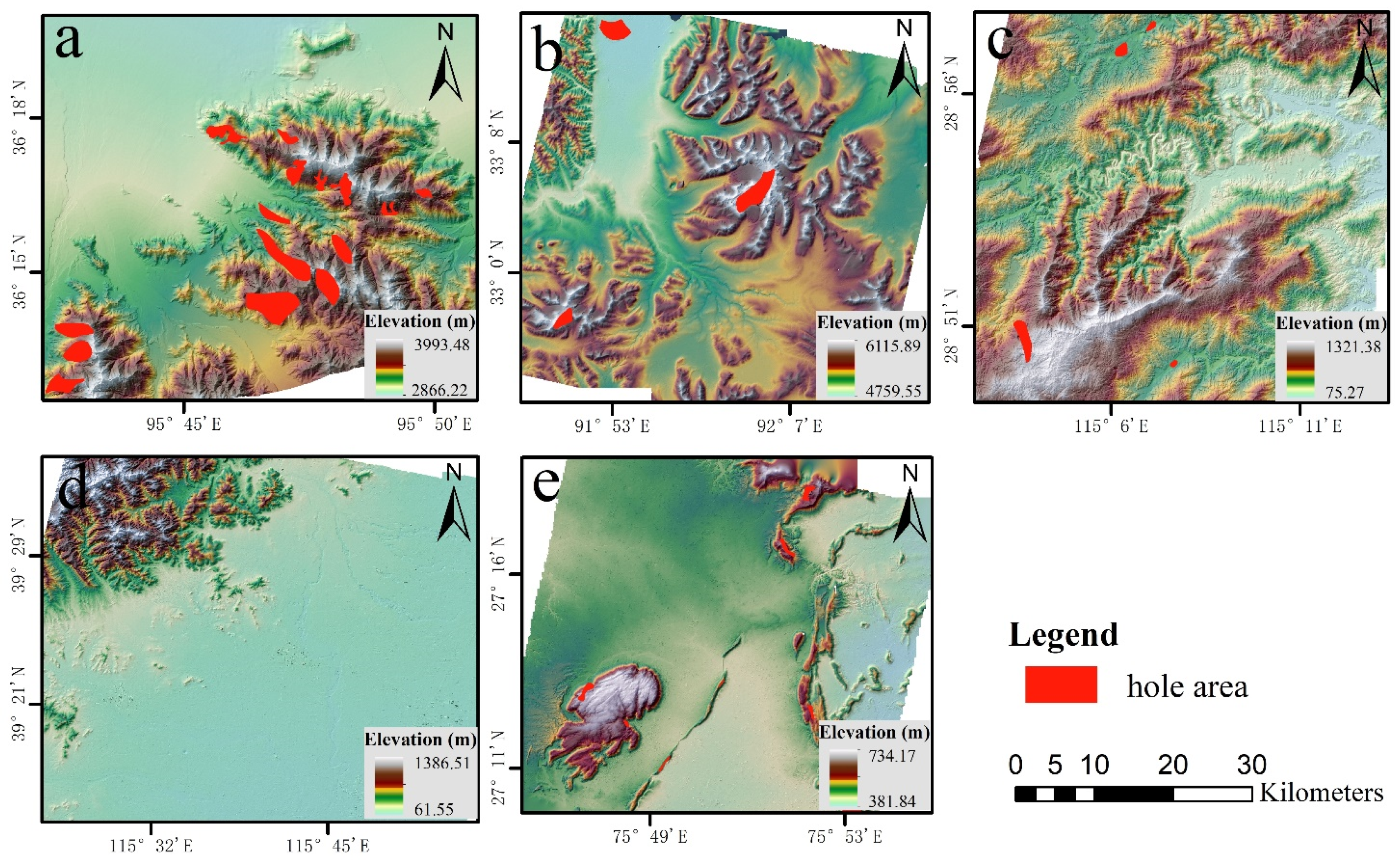
2. Research Area and Materials
3. Method
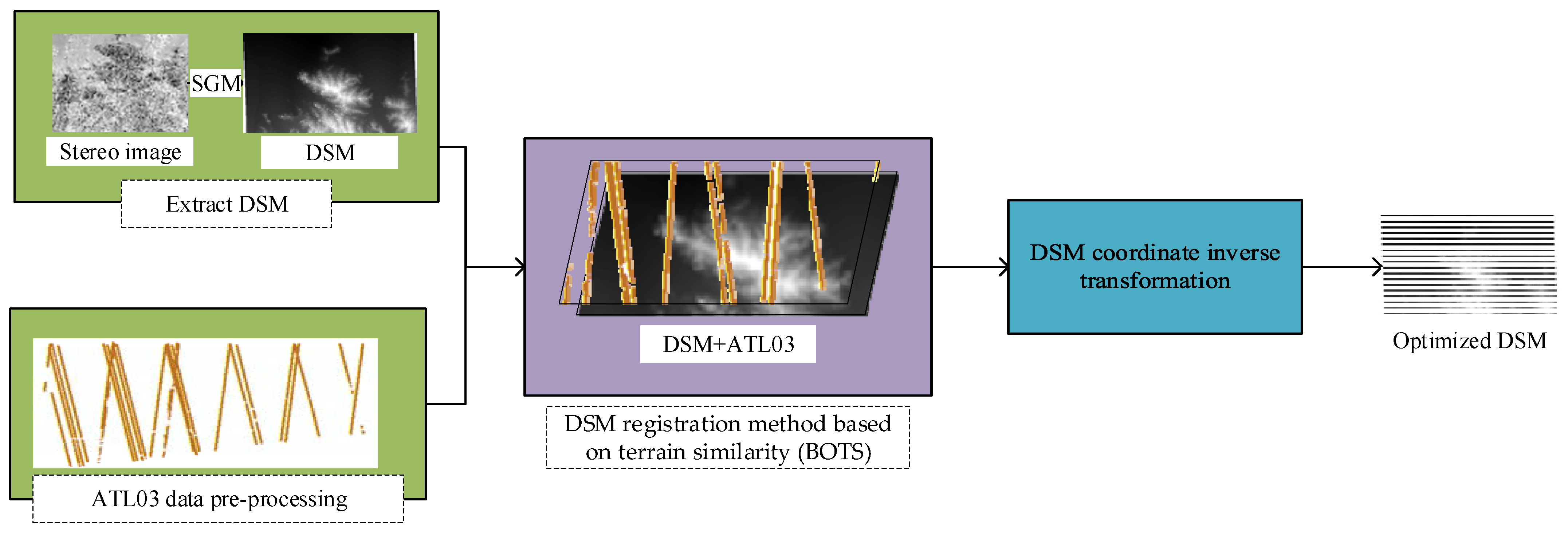
3.1. Algorithm Flow
- Step 1. Extract DSMCreate DSM with stereo images. The image geometry model adopts the rational function model (RFM). The output resolution is twice the image resolution. The DSM storage format is a regular grid, which is convenient for processing and calculation.
- Step 2. Data pre-processingExtract high-quality ATL03 photons and unify the spatial reference system among multisource data.
- Step 3. DSM registration based on terrain similarity (BOTS)Use DSM as the reference data and ATL03 as the source data to calculate the coordinate transformation parameters.
- Step 4. DSM coordinate inverse transformationTaking the DSM as the source data, use the calculated coordinate transformation parameters to inversely transform the coordinates of the DSM to improve the geometric accuracy of the DSM.
3.2. ATL03 Data Preprocessing
3.2.1. Photon Screening
3.2.2. Photon Classification
3.2.3. Photon Resampling
3.3. DSM Registration Method Based on Terrain Similarity
- (1)
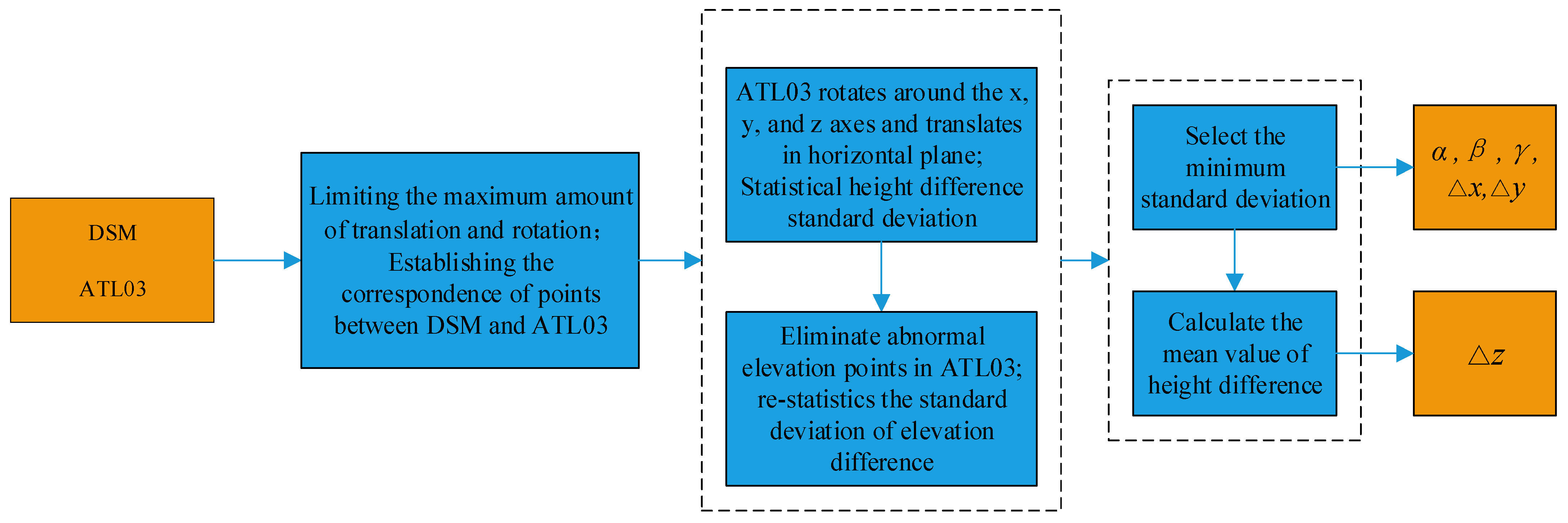
- Set the maximum translation and rotation amount. The purpose is to determine the range of horizontal movement, reduce unnecessary calculations, and improve registration efficiency. Determine the maximum horizontal moving distance by the remote sensing image accuracy and the horizontal accuracy of ICESat-2, which differs according to the image type.
- (2)
- Establish the corresponding point relationship. Use the coordinates of the ATL03 data to obtain the elevation values of these points on the DSM to form homonymous points. The height difference of homonymous points expresses the relationship between the two data sets.
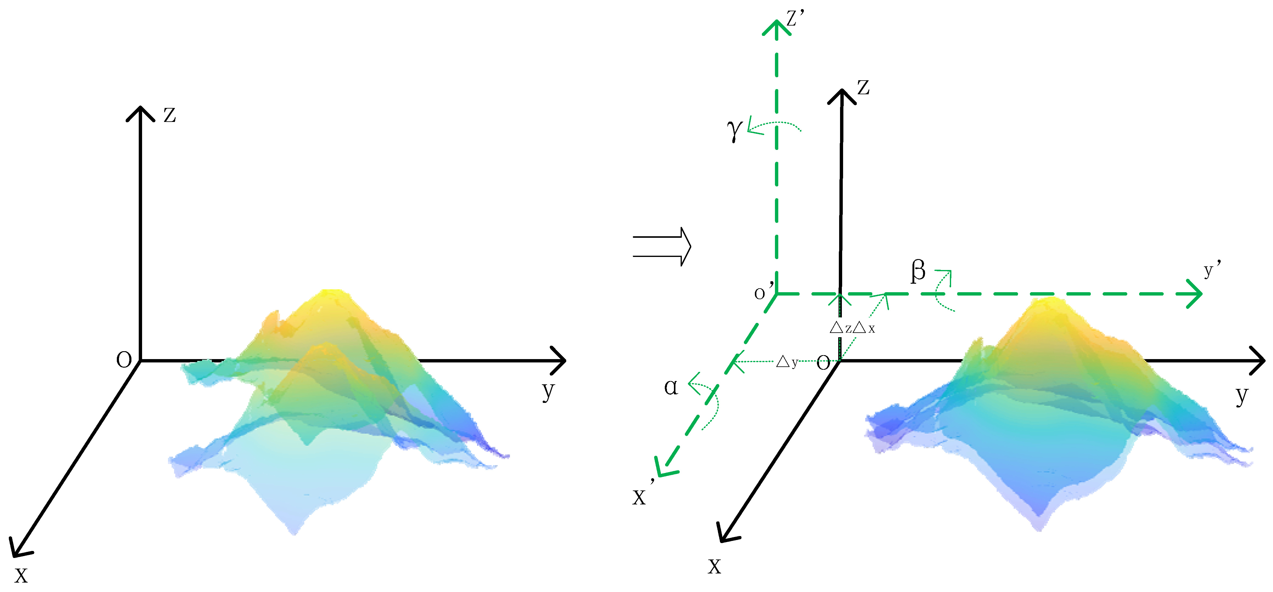
- (3)
- Using ATL03 as the source data set and satellite DSM as the reference data set, perform spatial rotation transformation around the x, y, and z axes, and perform the translation in the x-y plane. Calculate the transformed coordinate values according to Equation (1) and use Equations (2) and (3) to calculate the elevation difference standard deviation of all homonymous points.where HATL03 (i,j) and HDSM (i,j) are the elevations of the homonymous points formed by ATL03 and DSM, ∆h (i,j) is the elevation difference of homonymous points after each transformation, ∆H is the elevation difference set of homonymous points, i is the number of homonymous points, and j is the number of transformation times.where ∆hsd (j) is the elevation difference standard deviation of all homonymous points under the j-th spatial transformation of ATL03, and is the elevation difference standard deviation set of the homonymous points.
- (4)
- According to Equation (4), sequentially eliminate the abnormal elevation value data in the ATL03 data, calculate the standard deviation of the elevation difference of homonymous points again using Equations (5) and (6), and select the rotation when the standard deviation of the elevation difference is the smallest. Take the amount of translation as the optimal parameter value of α, β, γ, ∆x, ∆y. At this time, the mean value of the height difference when the standard deviation of the elevation difference is the smallest is calculated as the translation parameter ∆z in the z-axis direction.
4. Results
5. Discussion
5.1. Accuracy Analysis of BOTS Method
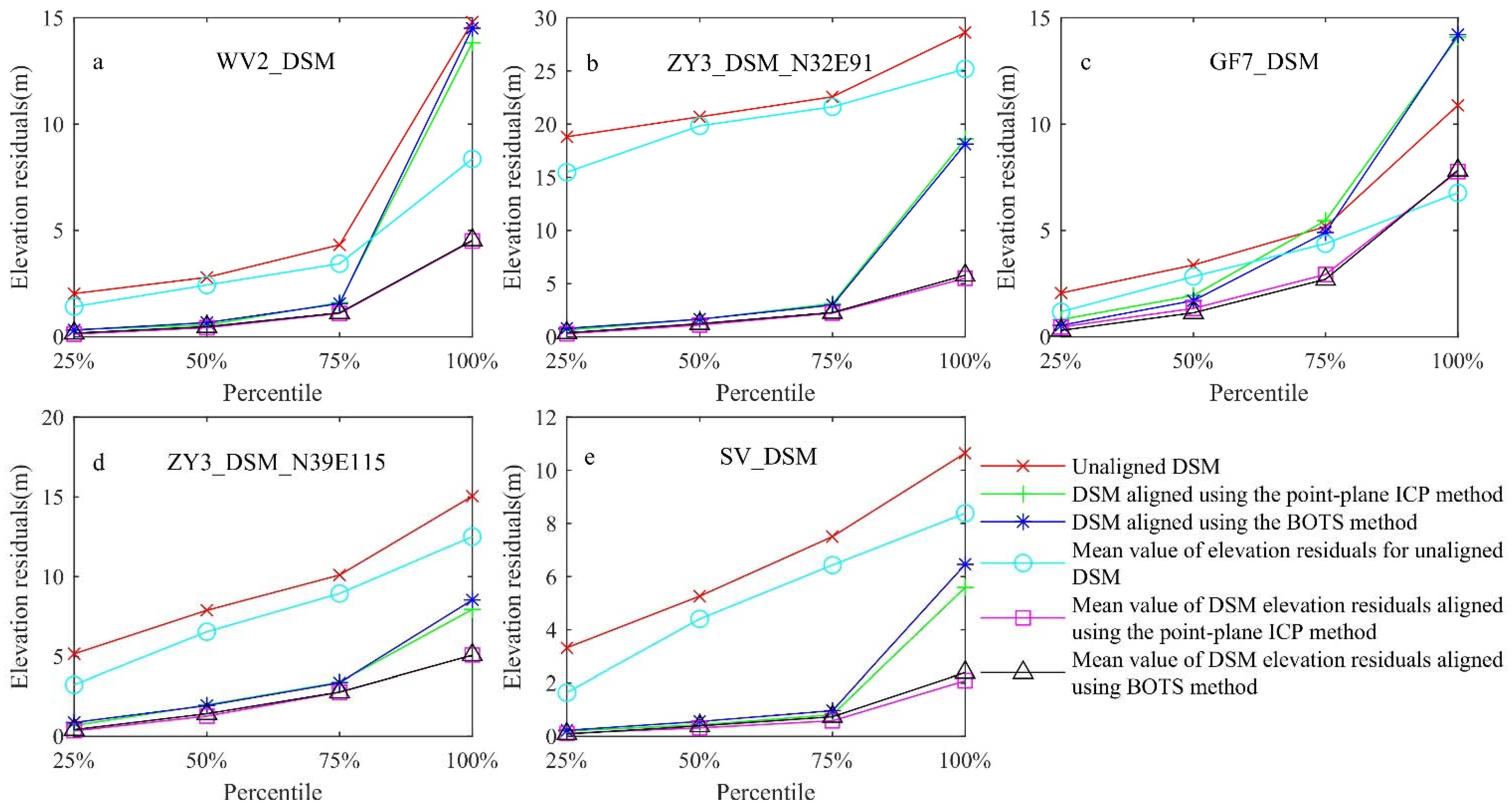
5.2. DSM Residual Error Distribution
6. Conclusions
Author Contributions
Funding
Institutional Review Board Statement
Informed Consent Statement
Data Availability Statement
Acknowledgments
Conflicts of Interest
References
- Girod, L.; Nuth, C.; Kääb, A.; McNabb, R.; Galland, O. MMASTER: Improved ASTER DEMs for Elevation Change Monitoring. Remote Sens. 2017, 9, 704. [Google Scholar] [CrossRef] [Green Version]
- Albino, F.; Smets, B.; d’Oreye, N.; Kervyn, F. High-resolution TanDEM-X DEM: An accurate method to estimate lava flow volumes at Nyamulagira Volcano (D. R. Congo). J. Geophys. Res. Solid Earth 2015, 120, 4189–4207. [Google Scholar] [CrossRef] [Green Version]
- Bisson, M.; Spinetti, C.; Andronico, D.; Palaseanu-Lovejoy, M.; Fabrizia Buongiorno, M.; Alexandrov, O.; Cecere, T. Ten years of volcanic activity at Mt Etna: High-resolution mapping and accurate quantification of the morphological changes by Pleiades and Lidar data. Int. J. Appl. Earth Obs. Geoinf. 2021, 102, 102369. [Google Scholar] [CrossRef]
- Kim, J.-W.; Lu, Z.; Qu, F.; Hu, X. Pre-2014 mudslides at Oso revealed by InSAR and multi-source DEM analysis. Geomat. Nat. Hazards Risk 2015, 6, 184–194. [Google Scholar] [CrossRef]
- Brun, F.; Berthier, E.; Wagnon, P.; Kääb, A.; Treichler, D. A spatially resolved estimate of High Mountain Asia glacier mass balances from 2000 to 2016. Nat. Geosci. 2017, 10, 668–673. [Google Scholar] [CrossRef] [PubMed]
- Cao, H.Y.; Liu, F.Q.; Zhao, C.G.; Dai, J. The study of high resolution stereo mapping satellite. Natl. Remote Sens. Bull. 2021, 25, 1400–1410. [Google Scholar] [CrossRef]
- Wang, J.; Wang, R.; Hu, X. Drift Angle Residual Corrrection Technology in Satellite Photogrammetry. Acta Geod. Cartogr. Sin. 2014, 43, 954–959. [Google Scholar] [CrossRef]
- Wang, J.; Wang, R.; Hu, X.; Su, Z. The on-orbit calibration of geometric parameters of the Tian-Hui 1 (TH-1) satellite. ISPRS J. Photogramm. Remote Sens. 2017, 124, 144–151. [Google Scholar] [CrossRef]
- Cao, J.; Yuan, X.; Gong, J.; Duan, M. The Look-angle Calibration Method for On-orbit Geometric Calibration of ZY-3 Satellite Imaging Sensors. Acta Geod. Cartogr. Sin. 2014, 43, 1039–1045. [Google Scholar] [CrossRef]
- Mi, L.D.W. A Review of High Resolution Optical Satellite Surveying and Mapping Technology. Spacecr. Recovery Remote Sens. 2020, 41, 1–11. [Google Scholar] [CrossRef]
- Anzhu, Y. Research on the Improvement of Georeferencing Accuracy of High Resolution Satellite Imagery; PLA Strategic Support Force Information Engineering University: Zhengzhou, China, 2017; Available online: http://cdmd.cnki.com.cn/Article/CDMD-90005-1018702170.htm (accessed on 1 June 2021).
- Jaud, M.; Passot, S.; Le Bivic, R.; Delacourt, C.; Grandjean, P.; Le Dantec, N. Assessing the Accuracy of High Resolution Digital Surface Models Computed by PhotoScan® and MicMac® in Sub-Optimal Survey Conditions. Remote Sens. 2016, 8, 465. [Google Scholar] [CrossRef] [Green Version]
- Ye, J.; Lin, X.; Xu, T. Mathematical modeling and accuracy testing of worldview-2 level-1B stereo pairs without ground control points. Remote Sens. 2017, 9, 737. [Google Scholar] [CrossRef] [Green Version]
- Markus, T.; Neumann, T.; Martino, A.; Abdalati, W.; Brunt, K.; Csatho, B.; Farrell, S.; Fricker, H.; Gardner, A.; Harding, D.; et al. The Ice, Cloud, and land Elevation Satellite-2 (ICESat-2): Science requirements, concept, and implementation. Remote Sens. Environ. 2017, 190, 260–273. [Google Scholar] [CrossRef]
- Babbel, B.J.; Parrish, C.E.; Magruder, L.A. ICESat-2 Elevation Retrievals in Support of Satellite-Derived Bathymetry for Global Science Applications. Geophys. Res. Lett. 2021, 48, 5. Available online: https://agupubs.onlinelibrary.wiley.com/doi/full/10.1029/2020GL090629 (accessed on 2 August 2021). [CrossRef] [PubMed]
- Chen, Y.; Zhu, Z.; Le, Y.; Qiu, Z.; Chen, G.; Wang, L. Refraction correction and coordinate displacement compensation in nearshore bathymetry using ICESat-2 lidar data and remote-sensing images. Opt. Express 2021, 29, 2411–2430. [Google Scholar] [CrossRef] [PubMed]
- Wang, S.; Alexander, P.; Wu, Q.; Tedesco, M.; Shu, S. Characterization of ice shelf fracture features using ICESat-2-A case study over the Amery Ice Shelf. Remote Sens. Environ. 2021, 255, 112266. [Google Scholar] [CrossRef]
- Lai, Y.R.; Wang, L. Monthly Surface Elevation Changes of the Greenland Ice Sheet From ICESat-1, CryoSat-2, and ICESat-2 Altimetry Missions. IEEE Geosci. Remote Sens. Lett. 2022, 19, 1–5. [Google Scholar] [CrossRef]
- Kwok, R.; Cunningham, G.F.; Kacimi, S.; Webster, M.A.; Kurtz, N.T.; Petty, A.A. Decay of the Snow Cover Over Arctic Sea Ice from ICESat-2 Acquisitions during Summer Melt in 2019. Geophys. Res. Lett. 2020, 47, e2020GL088209. [Google Scholar] [CrossRef]
- Liu, M.; Popescu, S.C.; Malambo, L. Feasibility of Burned Area Mapping Based on ICESAT-2 Photon Counting Data. Remote Sens. 2020, 12, 24. [Google Scholar] [CrossRef] [Green Version]
- Zhu, X.; Wang, C.; Nie, S.; Pan, F.; Xi, X.; Hu, Z. Mapping forest height using photon-counting LiDAR data and Landsat 8 OLI data: A case study in Virginia and North Carolina, USA. Ecol. Indic. 2020, 114, 106287. [Google Scholar] [CrossRef]
- Narine, L.L.; Popescu, S.C.; Malambo, L. Using ICESat-2 to Estimate and Map Forest Aboveground Biomass: A First Example. Remote Sens. 2020, 12, 1824. [Google Scholar] [CrossRef]
- Silva, C.A.; Duncanson, L.; Hancock, S.; Neuenschwander, A.; Thomas, N.; Hofton, M.; Fatoyinbo, L.; Simard, M.; Marshak, C.Z.; Armston, J.; et al. Fusing simulated GEDI, ICESat-2 and NISAR data for regional aboveground biomass mapping. Remote Sens. Environ. 2021, 253, 112234. [Google Scholar] [CrossRef]
- Sun, T.; Qi, J.; Huang, H. Discovering forest height changes based on spaceborne lidar data of ICESat-1 in 2005 and ICESat-2 in 2019: A case study in the Beijing-Tianjin-Hebei region of China. For. Ecosyst. 2020, 7, 704–715. [Google Scholar] [CrossRef]
- Li, W.; Niu, Z.; Shang, R.; Qin, Y.; Wang, L.; Chen, H. High-resolution mapping of forest canopy height using machine learning by coupling ICESat-2 LiDAR with Sentinel-1, Sentinel-2 and Landsat-8 data. Int. J. Appl. Earth Obs. Geoinf. 2020, 92, 102163. [Google Scholar] [CrossRef]
- Magruder, L.; Neuenschwander, A.; Klotz, B. Digital terrain model elevation corrections using space-based imagery and ICESat-2 laser altimetry. Remote Sens. Environ. 2021, 264, 112621. [Google Scholar] [CrossRef]
- Magruder, L.A.; Brunt, K.M.; Alonzo, M. Early ICESat-2 on-orbit Geolocation Validation Using Ground-Based Corner Cube Retro-Reflectors. Remote Sens. 2020, 12, 3653. [Google Scholar] [CrossRef]
- Bae, S.; Helgeson, B.; James, M.; Magruder, L.; Sipps, J.; Luthcke, S.; Thomas, T. Performance of ICESat-2 Precision Pointing Determination. Earth Space Sci. 2021, 8, e2020EA001478. [Google Scholar] [CrossRef]
- Luthcke, S.B.; Thomas, T.C.; Pennington, T.A.; Rebold, T.W.; Nicholas, J.B.; Rowlands, D.D.; Gardner, A.S.; Bae, S. ICESat-2 Pointing Calibration and Geolocation Performance. Earth Space Sci. 2021, 8, e2020EA001494. [Google Scholar] [CrossRef]
- Tian, X.; Shan, J. Comprehensive Evaluation of the ICESat-2 ATL08 Terrain Product. IEEE Trans. Geosci. Remote Sens. 2021, 59, 8195–8209. [Google Scholar] [CrossRef]
- Carabajal, C.C.; Boy, J.P. Icesat-2 altimetry as geodetic control. Int. Arch. Photogramm. Remote Sens. Spat. Inf. Sci. 2020, XLIII-B3-2020, 1299–1306. [Google Scholar] [CrossRef]
- Wang, M.; Wei, Y.; Yang, B.; Zhou, X. Extraction and Analysis of Global Elevation Control Points from ICESat-2 /ATLAS Data. Geomat. Inf. Sci. Wuhan Univ. 2021, 46, 184–192. [Google Scholar] [CrossRef]
- Yang, Q.; Wei, J.; Zheng, J.; Wang, R.; Jia, N.; Qiu, L. Comparison of interpolation methods of digital elevation model using discrete point cloud data. Sci. Surv. Mapp. 2019, 44, 16–23. [Google Scholar] [CrossRef]
- Besl, P.J.; McKay, N.D. A method for registration of 3-D shapes. IEEE Trans. Pattern Anal. Mach. Intell. 1992, 14, 239–256. [Google Scholar] [CrossRef]
- Rosenheim, D.; Torlegard, K. Three-Dimensional Absolute Orientation of Stereo Models Using Digital Elevation Models. Photogramm. Eng. Remote Sens. 1988, 54, 1385–1389. [Google Scholar]
- Zhang, T.; Cen, M.; Feng, Y. Comparison of LZD and ICP Algorithms in DEM Matching without Control Points. J. Image Graph. 2006, 11, 714–719. [Google Scholar] [CrossRef]
- Low, K.-L.; Lastra, A. Predetermination of icp registration errors and its application to view planning. In Proceedings of the Sixth International Conference on 3-D Digital Imaging and Modeling (3DIM 2007), Montreal, QC, Canada, 21–23 August 2007; pp. 73–80. [Google Scholar] [CrossRef]
- Neumann, T.; Brenner, A.; Hancock, D.; Robbins, J.; Saba, J.; Harbeck, K.; Gibbons, A.; Lee, J.; Luthcke, S. ATLAS/ICESat-2 L2A Global Geolocated Photon Data, Version 4; NASA National Snow and Ice Data Center Distributed Active Archive Center: Boulder, CO, USA, 2021. [CrossRef]
- Neumann, T.; Brenner, A.; Hancock, D.; Robbins, J.; Saba, J.; Harbeck, K.; Gibbons, A.; Lee, J.; Luthcke, S. ATLAS/ICESat-2 L2A Global Geolocated Photon Data, Version 3; NASA National Snow and Ice Data Center Distributed Active Archive Center: Boulder, CO, USA, 2020. [CrossRef]
- Khalsa, S.J.S.; Borsa, A.; Nandigam, V.; Phan, M.; Lin, K.; Crosby, C.; Fricker, H.; Baru, C.; Lopez, L. OpenAltimetry-rapid analysis and visualization of Spaceborne altimeter data. Earth Sci. Inform. 2020. [Google Scholar] [CrossRef]
- Hirschmuller, H. Accurate and efficient stereo processing by semi-global matching and mutual information. In Proceedings of the 2005 IEEE Computer Society Conference on Computer Vision and Pattern Recognition (CVPR’05), San Diego, CA, USA, 20–25 June 2005; Volume 802, pp. 807–814. [Google Scholar] [CrossRef]
- Neuenschwander, A.; Pitts, K.; Jelley, B.; Robbins, J.; Klotz, B.; Popescu, S.; Nelson, R.; Harding, D.; Pederson, D. ATLAS/ICESat-2 L3A Land and Vegetation Height, Version 4; NASA National Snow and Ice Data Center Distributed Active Archive Center: Boulder, CO, USA, 2021. [CrossRef]
- Dong, J.C.; Ni, W.J.; Zhang, Z.Y.; Sun, G.Q. Performance of ICESat-2 ATL08 product on the estimation of forest height by referencing to small footprint LiDAR data. Natl. Remote Sens. Bull. 2021, 25, 1294–1307. [Google Scholar] [CrossRef]
- Ghaderpour, E. Some equal-area, conformal and conventional map projections: A tutorial review. J. Appl. Geod. 2016, 10, 197–209. [Google Scholar] [CrossRef]
- Zabih, R.; Woodfill, J. Non-Parametric Local Transforms for Computing Visual Correspondence; Eklundh, J.-O., Ed.; Springer: Berlin/Heidelberg, Germany, 1994; pp. 151–158. [Google Scholar]
- Palaseanu-Lovejoy, M.; Bisson, M.; Spinetti, C.; Buongiorno, M.F.; Alexandrov, O.; Cecere, T. High-Resolution and Accurate Topography Reconstruction of Mount Etna from Pleiades Satellite Data. Remote Sens. 2019, 11, 2983. [Google Scholar] [CrossRef] [Green Version]
- Zhu, X.; Nie, S.; Wang, C.; Xi, X.; Hu, Z. A Ground Elevation and Vegetation Height Retrieval Algorithm Using Micro-Pulse Photon-Counting Lidar Data. Remote Sens. 2018, 10, 1962. [Google Scholar] [CrossRef] [Green Version]


| Study Area A | Study Area B | Study Area C | Study Area D | Study Area E | |
|---|---|---|---|---|---|
| Satellite | Worldview-2 | ZY-3 | GF-7 | ZY-3 | SuperView-1 |
| Spatial resolution | 0.46 m | Ndir: 2.1 m Front view: 2.5 m Back view: 2.5 m | Front view: 0.8 m Back view: 0.65 m | Ndir: 2.1 m Front view: 2.5 m Back view: 2.5 m | 0.5 m |
| Spectral band | Pan | Pan | Pan | Pan | Pan |
| Mapping accuracy without GCPs | horizontal: 2.3 m vertical: 5 m | horizontal: 10 m vertical: 5 m | horizontal: 7.2 m | horizontal: 10 m vertical: 5 m | horizontal: 9.5 m |
| Additional files | RPC | RPC | RPC | RPC | RPC |
| Heading | Number of Checkpoints | RMSE of Original DSM Elevation (m) | RMSE of DSM after BOTS Method Registration (m) | Increase Rate (%) |
|---|---|---|---|---|
| WV2_DSM | 92 | 2.6 | 0.7 | 73% |
| SV_DSM | 84 | 4.7 | 0.5 | 89% |
| GF7_DSM | 81 | 3.1 | 1.8 | 43% |
| ZY3_DSM_N32E91 | 213 | 19.2 | 1.6 | 92% |
| ZY3_DSM_N39E115 | 125 | 6.7 | 1.8 | 73% |
| DSM | Spatial Resolution | The Amount of Translation of the DSM Geometric Center in the Horizontal Direction | Difference of Translation Amount | ||||
|---|---|---|---|---|---|---|---|
| BOTS Method | ICP Method | ||||||
| North | East | North | East | ∆N | ∆E | ||
| WV2_DSM | 1 × 1 | 0 | 7.0 | 0.1 | 6.9 | −0.1 | 0.1 |
| SV_DSM | 1.5 × 1.5 | −4.5 | 13.5 | −4.7 | 12.7 | 0.2 | 0.8 |
| GF7_DSM | 1.5 × 1.5 | −1.5 | −6.0 | −0.6 | −5.3 | −0.9 | −0.7 |
| ZY3_DSM_N32E91 | 5 × 5 | −15.0 | 10.0 | −11.3 | 11.0 | −3.7 | −1.0 |
| ZY3_DSM_N39E115 | 5 × 5 | 5.0 | 0 | 5.0 | −1.8 | 0 | 1.8 |
| DSM | Using ICP-Aligned DSM (RMSE) | Using BOTS-Aligned DSM (RMSE) | RMSE Difference between BOTS and ICP |
|---|---|---|---|
| WV2_DSM | 0.678 | 0.71 | 0.031 |
| SV_DSM | 0.397 | 0.497 | 0.1 |
| GF7_DSM | 1.964 | 1.771 | −0.192 |
| ZY3_DSM_N32E91 | 1.497 | 1.556 | 0.059 |
| ZY3_DSM_N39E115 | 1.796 | 1.848 | 0.051 |
Publisher’s Note: MDPI stays neutral with regard to jurisdictional claims in published maps and institutional affiliations. |
© 2021 by the authors. Licensee MDPI, Basel, Switzerland. This article is an open access article distributed under the terms and conditions of the Creative Commons Attribution (CC BY) license (https://creativecommons.org/licenses/by/4.0/).
Share and Cite
Ye, J.; Qiang, Y.; Zhang, R.; Liu, X.; Deng, Y.; Zhang, J. High-Precision Digital Surface Model Extraction from Satellite Stereo Images Fused with ICESat-2 Data. Remote Sens. 2022, 14, 142. https://doi.org/10.3390/rs14010142
Ye J, Qiang Y, Zhang R, Liu X, Deng Y, Zhang J. High-Precision Digital Surface Model Extraction from Satellite Stereo Images Fused with ICESat-2 Data. Remote Sensing. 2022; 14(1):142. https://doi.org/10.3390/rs14010142
Chicago/Turabian StyleYe, Jiang, Yuxuan Qiang, Rui Zhang, Xinguo Liu, Yixin Deng, and Jiawei Zhang. 2022. "High-Precision Digital Surface Model Extraction from Satellite Stereo Images Fused with ICESat-2 Data" Remote Sensing 14, no. 1: 142. https://doi.org/10.3390/rs14010142