Article

Inter-Zone Differences of Convective Development in a Convection Outbreak Event over Southeastern Coast of China: An Observational Analysis

1
Xiamen Key Laboratory of Straits Meteorology, Xiamen Meteorological Bureau, Xiamen 361012, China
2
State Key Laboratory of Marine Environmental Science, College of Ocean and Earth Sciences, Xiamen University, Xiamen 361102, China
3
State Key Laboratory of Numerical Modeling for Atmospheric Science and Geophysical Fluid Dynamics (LASG), Institute of Atmospheric Physics, Chinese Academy of Sciences, Beijing 100029, China
4
Department of Atmospheric Sciences, National Taiwan University, Taipei 106319, Taiwan
*
Author to whom correspondence should be addressed.
Remote Sens. 2022, 14(1), 131; https://doi.org/10.3390/rs14010131
Submission received: 11 November 2021 / Revised: 11 December 2021 / Accepted: 21 December 2021 / Published: 29 December 2021
(This article belongs to the Special Issue Remote Sensing of Clouds and Precipitation at Multiple Scales)

Abstract

:
Among the densely-populated coastal areas of China, the southeastern coast has received less attention in convective development despite having been suffering from significantly increasing thunderstorm activities. The convective complexity under such a region with extremely complex underlying and convective conditions deserves in-depth observational surveys. This present study examined a high-impact convection outbreak event with over 40 hail reports in the southeastern coast of China on 6 May 2020 by focusing on contrasting the convective development (from convective initiation to supercell occurrences) among three adjacent convection-active zones (north (N), middle (M), and south (S)). The areas from N to S featured overall flatter terrain, higher levels of free convection, lower relative humidity, larger convective inhibition, more convective available potential energy, and greater vertical wind shears. With these mesoscale environmental variations, distinct inter-zone differences in the convective development were observed with the region’s surveillance radar network and the Himawari-8 geostationary satellite. Convection initiated in succession from N to S and began with more warm-rain processes in N and M and more ice-phase processes in S. The subsequent convection underwent more vigorous vertical growth from N to S. The extremely deep convection in S was characterized by the considerably strong precipitation above the freezing level, echo tops of up to 18 km, and a great amount of deep (even overshooting) and thick convective clouds with significant cloud-top glaciation. Horizontal anvil expansion in convective clouds was uniquely apparent over S. From N to S, more pronounced mesocyclone and weak-echo region signatures indicated high risks of severe supercell hailstorms. These results demonstrate the strong linkage between the occurrence likelihood of severe convection and associated weather (such as supercells and hailstones) and the early-stage convective development that can be well-captured by high-resolution observations and may facilitate fine-scale convection nowcasting.

Graphical Abstract

1. Introduction

Convective development is a complex function of moisture, instability, lift, and vertical wind shear that is governed by multiscale processes (e.g., [1,2]) and may show considerable variations in response to different combinations of these factors [3]. The complex nature of convective development undoubtedly increases the difficulty in convection nowcasting, particularly in terms of the location and timing of convective initiation (e.g., [4]) and the severity of convective storms (e.g., [5]). It is thus of great practical importance to glean a more comprehensive understanding of convective development across different scales (e.g., synoptic and storm scales), which fundamentally relies on thorough observational surveys.
Ground-based Doppler weather radars and geostationary meteorological satellites have been widely recognized as the most capable platforms to characterize convective processes. Radars capture the nature of convective precipitation by providing data of reflectivity (Z), radial velocity (Vr), and spectrum width (W). These data have been widely used to diagnose convective initiation (e.g., [6,7]), storm evolution (e.g., [8,9]), and wind field features (e.g., [10,11]). Additionally, radar-derived signatures, such as vertically integrated liquid water content (VIL), three-body scatter signature (TBSS), and mesocyclones, are known to be good indicators of severe convective storms or weather [12,13,14]. Unlike radars, geostationary satellites provide rapid-refresh cloud-top information for developing convective clouds, often involving newborn cumulus clouds preceding the radar-detected convective precipitation [15]. Mecikalski and Bedka [6] developed an “interest field” technique by processing multispectral data from the Geostationary Operational Environmental Satellite (GOES) to quantify convective cloud growth before convective initiation. Recently, other fields have been explored with additional spectral channels from more advanced geostationary satellites to describe various cloud-top features [16,17] and have been applied in determining not only convective initiation [18,19,20] but also storm evolution [21,22] and severity [5,23].
Numerous efforts based on radar and satellite observations have been made to reveal distinct convective characteristics across different climate regimes. When applying interest fields to nowcast convective initiation, Walker et al. [18] found that the algorithm performance varied among four independent regions across the U.S., which they partly attributed to the interregional differences in cloud growth rate and warm-rain processes resulting from differential instability and moisture content. Mecikalski et al. [24] analyzed both radar data and GOES interest fields, and they suggested that the convective growth before lightning initiation is less vigorous and dominated by more warm-rain processes in Florida relative to Oklahoma, where the environment is drier and more unstable. Chen et al. [25] showed variations in radar-observed convective initiation, growth, and organization modes with different prevailing wind regimes over contiguous North China. Huang et al. [26] conducted a satellite-based statistical survey that uncovered diverse cloud growth processes related to convective initiation over different landscapes and months over Central Eastern China. Such climatological variations in convective properties have also been deduced from Tropical Rainfall Measuring Mission (TRMM) observations (e.g., [27,28,29,30]), though the observations have been unable to capture the actual convective evolution. Overall, these studies can provide a general picture of convective features for specific climate regimes across the globe. These climatological convective features can also help understand the impacts of climate change on weather and precipitation extremes as relevant factors vary [31,32,33,34]. Beyond the climatological perspective, however, the detailed features in convective development associated with environmental variations on smaller scales (e.g., mesoscale) within a regime require further investigation, which may be more beneficial to fine-scale convection nowcasting.
The southeastern coast of China (Figure 1a), located to the west of the Taiwan Strait, is an ideal region for investigating the complexity of convective development on small scales due to its extremely complex underlying surfaces mainly distinguished by wide coastal mountains at multiple altitudes. Convective development in this region can be also complicated by the interaction between midlatitude and subtropical weather systems, especially during the transition between cold and warm seasons. Previous climatology studies have suggested that this region has been suffering a lot from severe convective weather (e.g., lightning; [35]), just as many other coastal regions in China with dense population do, and thunderstorm activities have been significantly increasing in this region [36]. However, studies of detailed convective characteristics, by well exploiting high-resolution observations, have been lacking in this complex region compared to other convection-active and densely-populated areas of coastal China (the southern coast of China is maybe the most studied one, e.g., [37,38]). Furthermore, observational evidence on the linkage between early-stage convective development and subsequent storm severity is insufficient in the southeastern coast of China, which has a subtropical climate regime. These issues largely motivated this study.
On 6 May 2020, a convection outbreak event hit the southeastern coast of China. It was the first high-impact severe weather event over this region after the onset of the 2020 warm season, and it was impressive for its production of more than 40 hail reports in the afternoon in addition to short-duration heavy rainfall (over 50 mm h−1) and dense lightning. The convection outbreak featured the successive development of multiple supercells in three adjacent zones (Figure 1b). Supercell outbreak events with intensive hail reports have been rarely documented in this region. This study was aimed to compare the convective features among these adjacent zones from the beginning of first convection until supercell occurrences. It differs from other studies (e.g., [39]) who also compared the convective features between nearby supercell storms but just focused on the relatively mature stage of the storms (e.g., cloud-top brightness temperature lower than 235 K). It is envisioned that the distinct features in the early stages of convective development may be related to subsequent storm severities and aid the early warning of severe weather.
In this study, comparisons were evaluated by jointly using observations from the region’s surveillance radar network and the Himawari-8 geostationary satellite from the perspectives of both precipitation and cloud. For complete comparisons, we explored the usage of all the three base moments (i.e., Z, Vr, and W) from the radar network observations. In particular, a new quantity derived from three-dimensional Z data is proposed to estimate the weak-echo region signature in convective storms. Multispectral interest fields derived from Himawari-8, a state-of-the-art geostationary satellite [40], were considered to cover the various cloud properties including cloud-top height, cloud optical thickness, cloud-top glaciation, particle size, and updraft strength. The combined utilization of radar- and satellite-based signatures to examine the convective initiation and growth processes in the southeastern coast of China could serve as a supplement to the limited number of relevant studies in the U.S. [24] and equatorial Africa [41].
The data used and their processing procedures are detailed in Section 2. Section 3 provides an overview of the convection outbreak event. Section 4 presents the observational differences in convective development among the three convection-active zones. Some issues are discussed in Section 5. Finally, conclusions are provided in Section 6.

2. Materials and Methods

This section presents the multisource data used in this study and the related methodology. The methodological framework for the two key remote sensing datasets used (radar and satellite datasets) is illustrated in Figure 2 and detailed as follows.

2.1. Multiple Radar Data and Their Processing Procedures

The radar data used in this study were collected by five operational radars belonging to China’s New Generation Doppler Weather Radars (CINRAD) network, along or near the southeastern coast of China (black squares in Figure 1a). All the radars have a wavelength of 10 cm (S-band) and a beam width of 1°. They operate in the VCP21 (volume coverage pattern 21) scanning mode, which takes approximately 6 min to complete a volume scan consisting of nine elevations between 0.5° and 19.5°. The three moments, i.e., Z, Vr, and W, were obtained with radial resolutions of 1, 0.25, and 0.25 km, respectively. A quality control procedure based on high-resolution terrain and W information was performed to remove the contaminated Z data due to ground and mountain clutters. The multiple radar data were mosaicked within a 6 min interval timeframe from 1200 local standard time (LST; LST = UTC + 8 h); for example, if the radar scan time was 1311 LST, then it fell into the closest 6 min time interval, i.e., 1312 LST, in the timeframe. The combination of the five radars provided a more intensive three-dimensional set of observations over the three zones than any single radar (Figure 1a), thus ensuring the reliability of the radar-based comparative results.
The mosaicked radar data were used to examine the convective characteristics via time–height diagrams and contoured frequency by altitude diagrams (CFADs). A time–height diagram shows the vertical (at 0.5 km intervals) distribution of a given variable as a function of time. CFADs display the frequency distribution of Z within a Z bin width (5 dBZ here) and a vertical interval (0.5 km here). They are often used for the composite analysis of individual storms (e.g., [24]), and they were used here to analyze the convective features within each convection-active zone as a whole. The mosaicked Z data were uniformly interpolated onto a 0.01° × 0.01° grid to produce the maximum Z image (vertical maximum in a grid) and derive the VIL and its density (the VIL divided by the echo top), according to Amburn and Wolf [12].
The TBSS and Doppler velocity dipole signatures were manually identified using Gibson-Ridge Analyst, version 2 (GR2Analyst 2.0; http://www.grlevelx.com/gr2analyst_2/, accessed on 22 May 2021). The TBSS is a region of relatively low Z that is radially aligned downrange from a high-Z core, often with near-zero Vr and noisy and overall large W [13]. Doppler velocity dipoles were determined in storm-relative velocity images when both the absolute values of outbound and inbound Doppler velocity maxima (Vr,max and Vr,min) were no less than 8 m s−1. For a velocity dipole, the rotational velocity was estimated as (Vr,maxVr,min)/2, and the azimuthal shear was estimated as (Vr,maxVr,min)/D, where D is the distance between Vr,max and Vr,min [42].

2.2. Himawari-8 Interest Fields

Observations from the Advanced Himawari Imager (AHI) onboard Himawari-8, the Japanese next-generation geostationary meteorological satellite [40], were used to derive the interest fields for describing cloud-top properties (or convective environments if cloudless). Himawari-8 is located at 140.7°E and thus has a good field of view of the study area. AHI is a multispectral (16-band) imager with 3 visible bands, 3 near-infrared bands, and 10 infrared bands. These bands have a central wavelength ranging from 0.47 to 13.3 μm, a spatial resolution at nadir between 0.5 and 2 km, and a full-disk scan interval of 10 min. In this study, we used the data with the 2 km spatial resolution for all bands, which are available via the P-Tree system of the Japan Aerospace Exploration Agency (https://www.eorc.jaxa.jp/ptree/index.html, accessed on 13 May 2021).
Based on the 16 AHI bands, a large number of interest fields are available in principle. However, many of them contain redundant information, as demonstrated in previous studies [16,17,19]. Accordingly, only six interest fields were selected in this study to describe various cloud-top properties, as summarized in Table 1. The 3.9 μm reflectance was derived from the 3.9, 10.4, and 13.3 μm brightness temperatures to remove the thermal emission portion [19,43]. Note that all the visible and near-infrared reflectances were normalized by the solar zenith angle (θ) by 1/cosθ. When considering the cloud-top properties based on the interest fields, a cloud mask was performed to discard clear-sky pixels by using a visible (0.47 μm) reflectance of less than 30%.

2.3. Other Datasets

Some additional datasets were used to examine the synoptic conditions and convective environment. They included 5 min surface observations from automatic weather stations in Fujian province and radiosonde observations at Xiamen and Fuzhou (red triangles in Figure 1a) operated by the China Meteorological Administration, hourly 0.25° × 0.25° ERA5 reanalysis data from ECMWF [44], and 1 arc-min gridded elevation and bathymetry ETOPO1 data from the U.S. National Geophysical Data Center [45].
Table 1. List of Himawari-8 interest fields selected in this study to demonstrate convective development in light of cloud-top properties, along with their definitions and physical description.
Interest FieldDefinitionPhysical Description
ρ0.470.47 μm (band 1) reflectanceCloud optical thickness
ρ3.93.9 μm (band 7) reflectanceCloud-top glaciation, particle size
BTD6.2−7.3Brightness temperature difference between 6.2 (band 8) and 7.3 (band 10) μmCloud-top height relative to upper troposphere
BT10.410.4 μm (band 13) brightness temperatureCloud-top height
BTD12.4−10.4Brightness temperature difference between 12.4 (band 15) and 10.4 (band 13) μmCloud optical thickness
Trispectral differenceBrightness temperature difference between 8.6 (band 11) and 11.2 (band 14) μm minus brightness temperature difference between 11.2 (band 14) and 12.4 (band 15) μmCloud-top glaciation

3. Overview of Convection Outbreak Event

On 6 May 2020, the convection outbreak event started right after midday and gradually dissipated into the night. The convective activities occurred at the northern periphery of the western Pacific Subtropical High (Figure 3a,b). The subtropical high center (≥5880 gpm region) dominated the southern part of the study domain and apparently moved southward over the course of convection outbreak. The northern part of the study domain was invaded by relatively cold air mass at lower troposphere (corresponds to the higher sea level pressures in Figure 4b), which was likely propagated by the northeasterly wind associated with the offshore low vortex (Figure 3a,b). The northeasterly moist (more approaching saturation) and cold air mass interacted with the southwesterly dry and warm air mass under the control of the subtropical high, resulting in a north–south-orientated shear line with large gradients in both temperature and humidity at lower levels (Figure 3c–e and Figure 4a). Locally enhanced vertical motions could also be seen nearby the shear line. These heterogeneous synoptic conditions may have contributed to different convective developments over the study domain.
Along the southeastern coast of China, the convective environment appeared to be more unstable from north to south, as demonstrated by a modified convective available potential energy (CAPE) from Xiamen sounding (as a reference for the south; Figure 5a) that was ~20% higher than that from Fuzhou sounding (as a reference for the north; Figure 5b). The environmental soundings also showed a higher level of free convection (LFC) and larger convective inhibition (CIN) in the south than in the north. The vertical wind shears for convection to develop were estimated based on the soundings’ wind profiles at 08 LST while replacing the near-surface winds with in situ 10 m winds at 1200 LST (Figure 4b). Likely due to the sea-breeze effect, there was a low-level wind shift in the south from westerly wind in the early morning (Figure 5a) to easterly wind as solar insolation was enhanced (Figure 4b) (also seen in wind profile radar and Doppler Vr images, which are not shown here). As a result, the vertical wind shears were larger in the south than in the north. For example, the surface-to-500-hPa (approximately 0–6 km) bulk wind difference at 1200 LST was ~21.2 m s−1 at Xiamen station (Figure 5a) versus 16.6 m s−1 at Fuzhou station (Figure 5b).
Figure 3. ERA5 reanalysis of geopotential heights (gpm) at 500 (black contour lines) and 850 hPa (shaded) at (a) 1200 and (b) 1400 LST. ERA5 reanalysis of winds (full bar = 4 m s−1; half bars = 2 m s−1), temperatures (°C; shaded), and relatively humidity (%; green contour lines—only 75%, 85%, and 95% contour lines are shown) at 850 hPa at (c) 1200 and (d) 1400 LST. (e) Cross-section showing temperatures (°C; shaded), relatively humidity (%; green contour lines), and winds (m s−1 for horizontal velocity and Pa s−1 for vertical velocity; vectors) along the magenta line in (c). The blue triangles in (c,d) denote the shear line location estimated by the local maxima of 850 hPa temperature gradients. The vertical velocity in (c) is multiplied by 10 for visualization.
Remotesensing 14 00131 g003
Figure 4. In situ surface weather observations of (a) 2 m temperatures (°C; shaded) and dewpoint depression (°C; green contour lines), (b) 10 m winds (direction is shaded and speed is indicated by circle size) and sea level pressure (blue lines) at 1200 LST. The dewpoint depression in (a) and sea level pressure in (b) were interpolated onto a 0.01° × 0.01° grid using the Cressman interpolation scheme [46]. Three convection-active zones are indicated by the black boxes.
Remotesensing 14 00131 g004
Figure 5. Skew-T log-P diagrams of the (a) Xiamen and (b) Fuzhou radiosondes (station locations given in Figure 1a) at 08 LST on 6 May 2020. The ambient temperature and dew point are, respectively, represented by the solid black and green lines. To obtain more representative pre-convective environments, the Xiamen and Fuzhou soundings were modified by assuming a well-mixed boundary layer using the mean surface values at the stations within the south and north convection-active zones (as in Figure 4a) at 1200 LST, respectively. The modified ambient temperatures are plotted as black dashed lines. The parcel ascent (undiluted from the surface) curves without and with sounding modification are indicated by the solid and dashed red lines, respectively. The wind profile is shown on the left side of each panel (full bar = 4 m s−1; half bars = 2 m s−1; flag = 20 m s−1). The surface-based convective available potential energy (CAPE), convective inhibition (CIN), and level of free convection (LFC) values were calculated using both the original and modified (shown in parentheses) soundings. The surface-to-500-hPa vertical wind shear (VWS) at 1200 LST was estimated based on the soundings’ wind profiles at 08 LST while replacing the near-surface winds with in situ 10 m winds at 1200 LST (Figure 4b).
Remotesensing 14 00131 g005
As seen in the sequence of radar mosaics (refer to Figure 6), the convection outbreak was characterized by successive occurrence of convective cells after its onset. Interestingly, the early-stage convective activities (i.e., Z ≥ 35 dBZ) were concentrated in three individual but adjacent areas from north to south, with a maximum center distance of less than 200 km (Figure 1b). There were also three heavy rainfall centers with maximum hourly rainfall of more than 20 mm near the three convection hotspots (Figure 1b). For the comparison analysis, three zones with almost equal areas were selected to cover the convection hotspots: the north (N; 118.0°–119.2°E, 25.5°–26.1°N), middle (M; 117.4°–118.6°E, 24.8°–25.4°N), and south (S; 117.1°–118.3°E, 24.2°–24.8°N) zones (Figure 1). The study period began at 1200 LST, before the convective initiation in all zones, and it ended at 1500 LST, after which some of the mature convective cells in different zones tended to merge together. A preliminary investigation showed the occurrence frequency of strong convection (e.g., Z ≥ 50 dBZ) and hail report number during the study period were different between zones (Figure 1b). This implies that the convective development of this convection outbreak might have distinct features in different zones, which are investigated in detail based on radar and satellite observations in next section.

4. Inter-Zone Comparison Results of Convective Development

4.1. Features of Convection and Precipitation: Three-Dimensional Radar Analyses

The comparison of the convective development among the three convection-active zones began with the radar analyses in terms of initial convection, subsequent convective development, and evolutions of vertical structure and supercell-related signatures.

4.1.1. Initial Convection

Convective activities appeared in turn from N to S. The initiation of the first convection, defined as the first occurrence of continuous aloft Z ≥ 35 dBZ [15], was observed at 1218, 1236, and 1248 LST in N, M, and S, respectively (Figure 7a1–c1). The CFADs at 1230 LST (Figure 8a1–c1) show that the N convection had mean (maximum) Z values exceeding 0 (35) dBZ at an uppermost altitude of ~9.5 (6) km, while there were barely any mean (maximum) Z values exceeding 0 (35) dBZ above the surface for M and S. From north to south, a less saturated environment (Figure 3c–e and Figure 4a) with a higher LFC and larger CIN (Figure 5) made convective initiation significantly more difficult and thus occur later. The convection originated from the mountainous areas in M and N and the coastal plain in S (Figure 1b). The interaction between the southwestward-moving shear line (Figure 3c,d) and high terrain may have acted as a triggering mechanism for the convective initiation in N and M.
After initiation, the ≥50 dBZ strong convective precipitation (SCP) appeared immediately (within ~6 min) in N and S, but it did not appear in M until ~42 min later (Figure 7a2–c2). Mainly occurring below the freezing level, the initial convection in M before 1318 LST was too shallow to produce SCP (Figure 7b1,b2). For N, the initial convection happening in a relatively moist environment (Figure 3c–e and Figure 4a) was dominated by warm-rain processes, with most SCP below the freezing level until ~1400 LST (Figure 7a2). The initial convection in S exhibited most explosive development once the relatively strong CIN (Figure 5a) was overcome, with the production of SCP extending into the −20 °C levels within 30 min from the convective initiation time (Figure 7c2). As seen in the CFADs, a rapid decrease in maximum Z with height from the freezing level upward was observed in the initial convection in N and M (refer to the outmost curves in Figure 8a1,a2,b2), again suggesting dominant warm-rain processes within weak updrafts [24,47]. In contrast, the deepest initial convection in S had a larger maximum Z within the mixed-phase layer (freezing to −20 °C levels) than other levels (Figure 8c2).

4.1.2. Subsequent Convective Development

The subsequent convection was overall more active from N to S in both the horizontal and vertical views, as evidenced by the higher occurrence frequency and altitude of Z ≥ 35 dBZ (maximum height from ~12 to 16 km; Figure 7a1–c1). The SCP was also more prevalent from N to S, especially with more frequent occurrences above the −20 °C level (Figure 7a2–c2), signifying a higher potential for producing severe convection and hail [48]. Within each zone, a larger magnitude in the maximum 5 min surface rainfall was observed as the radar-based SCP became more active (Figure 7a2–c2). It seems that higher occurrence frequency and altitude of SCP were required from N to S to achieve a surface rain rate of >5 mm (5 min)−1, likely due to the less saturated boundary layer (Figure 3c–e and Figure 4a). Convective intensity tended to increase from N to S, with overall larger maximum Z values and higher echo tops (uppermost height of the 20 dBZ echo) (Figure 7a3–c3). The echo top rapidly increased in S to achieve a height up to 18 km with a slope of ~1.7 m s−1 between 1248 and 1412 LST versus ~1.3 m s−1 in M and ~0.8 m s−1 in N during the same period (Figure 7a3–c3). These results imply a stronger updraft from N to S to support more vigorous convective development, which can be attributed to the larger CAPE from north to south (Figure 5).
Four representative times were selected to specify the convective growth processes (Figure 6). The convective development within each zone was characterized by increases in the number, horizontal area expansion, and maximum intensity of individual convective cells (Figure 6). This resulted in wider surface rainfall coverage, along with more intensive 5 min precipitation rates (i.e., more and larger black dots in Figure 6). The CFADs show that the convection within each zone also grew vertically, with more and larger Z values uplifted to higher altitudes (Figure 8). At 1418 LST, the uppermost altitude of mean (maximum) Z over 0 (35) dBZ extended to 13 (11.5), 14.5 (13.5), and 18 (16) km in N, M, and S, respectively (Figure 8a4–c4). From N to S, the sharper profile expansions again point to faster convective growth.
As convection grew in all zones, there was a tendency toward more dominant ice-phase processes (e.g., riming) to facilitate hail production, with an enhanced maximum frequency core (nearby the mean Z profile) above the freezing level (Figure 8). This was particularly true for S, where more large Z values appeared above the −20 °C level (Figure 8c3,c4). A negative slope of the core from ~11 to near 17 km in S at 1418 LST (refer to the black curve in Figure 8c4) indicates the presence of a large amount of small ice particles at the convective cloud tops [24], which was less apparent in other zones (Figure 8a4,b4). This may have been related to the fast occurrence and expansion of deep convective cloud anvils in S favored by the relatively large vertical wind shear (Figure 5a), and it is further discussed in the forthcoming analysis based on Himawari-8 interest fields.

4.1.3. Vertical Structure Evolution

More realistic vertical structures of convection can be explored from the VIL and its derivations. The VIL integrates Z throughout a whole vertical column and is thus more capable of distinguishing different components of convective systems relative to the maximum Z (see Figure 9a versus Figure 6c). Figure 9 shows an example at 1336 LST across a lofted deep convective core in S with a weak-echo region (WER) at low levels. WERs are associated with wide and strong updrafts and have been long recognized as indicators of severe storms (e.g., [14]). It was observed that the WER was located in columns where the VIL and its density were extremely high, the ratios of the VIL above the freezing and −20 °C levels were reasonably large, and the equivalent altitude (VIL-weighted altitude) was near the −20 °C level (dashed box in Figure 9b,c). For subsequent comparison, the WER was defined as the region with a VIL greater than 20 kg m−2 and a VIL ratio above the freezing level of more than 75%. This newly-defined WER quantity demonstrates a way to quantify the visibility of WER signatures by considering the vertical distribution of convective echoes within a storm.
There was a growing trend for the maximum VIL in each zone (Figure 10a), indicating enhanced convective depth and intensity. A maximum VIL larger than 25 kg m−2, which is a typical threshold used to indicate hail production (e.g., [49]), was achieved in S first from 1312 LST, followed by M from 1336 LST and N from 1418 LST. There were two clear, sharp growths in S, with ~80 kg m−2 increments during 1254–1324 LST and 1354–1412 LST. The growth was relatively steady in M, with an ~130 kg m−2 increment from 1318 to 1500 LST, and much slower in N, especially before 1412 LST. Similar results could be observed in the maximum VIL density (Figure 10b), except with smaller variations due to the normalization by the echo top. Notably, two peak values in S (at 1324 and 1412 LST) were more comparable in maximum VIL density (~7 and ~8 g cm−3, respectively) than in maximum VIL (~80 and ~140 kg m−2, respectively). This implies that the second growth in maximum VIL could have been largely contributed by the growth in convective echo top, as confirmed by Figure 7c3. The WER appeared earlier and had a larger area in S than in M and N over most of the period (Figure 10c). These features again demonstrate overall stronger updrafts from N to S.

4.1.4. Supercell-Related Signature Evolution

Cyclonically rotating vortex signatures were observed in succession from S to N (Figure 11). For each zone, these vortexes generally had a peak rotational velocity over 14 m s−1, a vorticity (twice the azimuthal shear) exceeding 10−2 s−1, a vertical extent more than 3 km above ground level, and a duration of more than 30 min, which met the mesocyclone criteria used to identify the presence of a supercell (e.g., [3,50]). From N to S, the mesocyclone formed sooner after the convective initiation, and it intensified faster to obtain higher vertical extent and stronger rotation (Figure 11). According to the mesocyclone strength nomogram [51], most mesocyclones in S could be categorized as strong mesocyclones, while there were weak to moderate mesocyclones (until 1436 LST) for M and weak shears to weak mesocyclones for N. At the midlevel near 6.5 km, the S rotational velocity reached a maximum of 34.75 m s−1 (red dot in Figure 11c), which was higher than the 75th percentile in the giant hail cases across the contiguous U.S. (~30 m s−1; [52]). In M and S, the maximum low-level (below 3 km) rotational velocity exceeded 26 m s−1 (Figure 11b,c), which was comparable with the median value for a supercell to produce EF2 tornadoes in the contiguous U.S. [53].
Large azimuthal shears were found to run ahead of the large rotational velocities in S (Figure 11c), which were more synchronous in N and M (Figure 11a,b), as well as in previous studies (e.g., [42]). This could be partly explained by a rapid rotation strengthening process caused by large azimuthal shears that led to larger rotational velocities. On the other hand, the mesocyclones in S might have broadened when they achieved larger rotational velocity, resulting in a smaller azimuthal shear.
Figure 11. Time–height diagrams of rotational velocity (circle color) and its related azimuthal shear (10−3 s−1; circle size), as well as the frequency (%) of large (≥5 m s−1) spectrum width (W; contour lines) for the (a) north, (b) middle, and (c) south zones. At the same time, only the maximum rotational velocity and its related azimuthal shear were retained for each zone. For the W frequency distribution, the time interval is 6 min and the height interval is 0.5 km. For each time interval, the frequencies were normalized by the total radar-detected echo number at each vertical interval and are presented as fractions. The red dashed lines indicate the freezing and −20 °C levels. The black triangles represent the convective initiation times.
Remotesensing 14 00131 g011
Interestingly, the higher-level (above the 0 °C level) large W values (≥5 m s−1) (HLW; contour lines in Figure 11) were observed to collocate well with the convective development (Figure 7) in each zone. We checked the radar images and found the HLW could mainly be attributed to wind shears (especially those near rotating vortexes), storm-top divergence, and turbulence within the TBSS region. Since all these factors are associated with severe convection, a more frequent HLW implies more active severe convection such as supercells. This was also confirmed by the in-phase variations of the HLW frequency (especially the 3% contour) and vortex strength in each zone (Figure 11). From N to S, the more frequent occurrence and higher vertical extent of HLW (Figure 11) again indicated a greater likelihood of strong convection. In the past, W has been applied the least among these three radar base moments, mainly because the always turbulent near-surface W shows little use for analyzing convection. However, the results of this analysis show that the high-level W is worthy of further exploration.

4.2. Convective Cloud Properties: Interpretations of Himawari-8 Interest Fields

Convective differences among the three zones were further considered in light of cloud-top properties by interpreting the Himawari-8 interest fields (Table 1). The field behaviors in each zone are presented via normalized frequency (i.e., fraction) distributions as a function of time.

4.2.1. Cloud-Top Height

Overall, the clouds achieved higher tops in S than in M and N. In the 10.4 μm BT (BT10.4) field, a lower value generally indicates a higher cloud top. The tendency toward the cold side in the BT10.4 distributions (Figure 12a–c) suggests increasing cloud-top heights in all zones. Nevertheless, more high-top clouds were seen in S, with approximately 25% of BT10.4 values lower than −60 °C (an equivalent altitude of ~14 km) after 1410 LST (Figure 12c). The coldest BT10.4 of less than −75 °C (near the tropopause temperature) in S (1410–1420 LST in Figure 12c) indicated a higher likelihood of an overshooting top near the convective core relative to M and N (refer to Figure 13c3). Note that such deep convective clouds in S developed from a more cloudless environment where the initial BT10.4 values were mostly warmer than 20 °C (Figure 12c) relative to N and M (Figure 12a,b) due to the impact of the subtropical high center (Figure 3a,b).
The fairly high cloud tops in S mainly resulted from the vigorous vertical growth around the updraft core in convective clouds. This was evidenced by the 30 min cooling magnitude of ~45 °C in minimum BT10.4 during 1240–1310 LST (topmost curve in Figure 12c). Such a cooling rate can be defined as “strong convective growth” according to Hartung et al. [54] (i.e., a cooling rate ≥20 °C (15 min)−1), which is more likely to produce larger maximum Z and VIL in the interior plains of the U.S. Indeed, both the maximum Z (Figure 7c3) and VIL (Figure 10a) in S were considerably large. The cooling trend was much gentler for N (topmost curve in Figure 12a) and even not robust for M until 1310 LST (topmost curve in Figure 12b), before which shallow convection prevailed (Figure 7b1–b3). The first remarkable vertical growth, represented by a cooling rate of ≥5 °C (10 min)−1, happened in N, M, and S at 1220, 1230, and 1240 LST, respectively, close to the radar-defined convective initiation times (i.e., 1218, 1236, and 1248 LST). In S, such remarkable cooling was accompanied by a drop in the minimum BT10.4 below 0 °C (blue triangle in Figure 12c), satisfying the common criterion used to nowcast midlatitude convective initiation [6,18] but offering a short lead time (~8 min) due to the more tropical environment here.
Horizontal anvil expansion in convective clouds can also result in a sudden increasing portion of cold BT10.4 values [22], which was observed here earlier and more overwhelmingly in S. The fraction of BT10.4 values lower than −40 °C (Figure 12c) was tiny before 1330 LST (see also Figure 13a2), but it then increased rapidly and exceeded 25% at 1350 LST (see also Figure 13a3), eventually peaking at 1440 LST with a magnitude near 50%. For N and M, the fraction was no more than 25% until 1440 and 1450 LST, respectively (Figure 12a,b), much later than in S. An earlier anvil formation and faster anvil expansion, which could have been related to the larger vertical wind shear (Figure 5), confirmed more vigorous convective development in S than in N and M.
The above cloud-top height results are supported by the BT difference (BTD) between 6.2 and 7.3 μm, which estimates the cloud-top height relative to the upper troposphere [55]. As clouds developed into the upper troposphere, BTD6.2−7.3 became less negative, and it approached and even exceeded 0 K. From 1240 LST onward, the maximum BTD6.2−7.3 in S quickly increased from a magnitude less than −17 K and became positive at 1330 LST (Figure 12f), signifying that the cloud had developed into the upper troposphere and even gained overshooting status through vigorous vertical growth. For M and N, the maximum BTD6.2−7.3 increased as well but did not exceed 0 K until 1400 (Figure 12e) and 1420 LST (Figure 12d), respectively (see also Figure 13b3). It was hard for convective clouds to develop further when they had approached the tropopause, as evidenced by the consistent maximum BTD6.2−7.3 values above 0 K for all zones (topmost curves in Figure 12d–f). However, the overall BTD6.2−7.3 kept increasing due to a larger portion of BTD6.2−7.3 values near 0 K (Figure 12d–f), which may have been closely related to the anvil expansion near the tropopause.

4.2.2. Cloud Optical Thickness

Among the three zones, S exhibited the most prominent cloud-thickening process and thus had the overall largest cloud optical thickness, as derived from the daytime 0.47 μm reflectance (ρ0.47). A thicker cloud produces a higher ρ0.47. At the beginning, from N to S, less variability in ρ0.47 could be seen (Figure 14a–c). Over 90% of the ρ0.47 values in S were below 30% at 1200 LST (Figure 14c). These results corroborate a more cloudless condition from N to S before the onset of convection, as derived from the BT10.4 field. With various thicknesses (30–90% ρ0.47; Figure 13c1) and relatively warm temperatures (BT10.4 > −10 °C; Figure 13a1), the initial clouds in N and M were likely to be low and thick clouds or high and thin clouds. After convective initiation, the convective clouds became thicker with increasing ρ0.47 values, which was more notable from N to S (Figure 14a–c). The maximum ρ0.47 in S approached 100% at 1320 LST and exceeded those in M and N (topmost curves in Figure 14a–c; see also Figure 13c2). Meanwhile, a larger group of clouds became thicker in S, with over 25% of ρ0.47 values larger than 80% from 1400 LST onward (Figure 14c).
The cloud thickness differences among zones are evidenced by the BTD12.4−10.4 field. The initial BTD12.4−10.4 values were overall more negative from N to S (Figure 13d1 and Figure 14d–f) due to the more cloudless condition. Dominated by faster convective growth, S inversely possessed larger BTD12.4−10.4 values produced by thicker clouds (Figure 14f). Approximately 25% of the values were greater than −2 K in S at 1350 LST (Figure 13d3 and Figure 14f), which was achieved much later in M (1440 LST in Figure 14e) and N (1430 LST in Figure 14d). In addition to the concentration center near −2 K, another one near −7 K after 1400 LST was observed for the clouds in S (Figure 14f) but was not obvious in N and M (Figure 14d,e). A similar bifurcated distribution of the cloudy pixels was seen in the ρ0.47 field in S, with a low-value center near 40% (Figure 14c). The low-value centers were likely associated with the storm anvil edges (refer to Figure 13c3,d3), where the clouds were often semitransparent (e.g., cirrus anvil; [56,57]) and their satellite-detected thickness could be partly reduced by the underlying surfaces. This was particularly true for S, where the convective storms underwent the most vigorous anvil expansion among the three zones.

4.2.3. Cloud-Top Glaciation

Cloud-top glaciation from condensed water clouds is a prerequisite for convective storms to produce hail [58], and it can be inferred by the trispectral difference of the 8.6, 11.2, and 12.4 μm BTs (e.g., [16]). Specifically, ice-top clouds have larger values in BTD8.6−11.2 than in BTD11.2−12.4 due to a faster increase in absorption coefficient between 8.6 and 11.2 μm than between 11.2 and 12.4 μm, while the reverse is true for water-top clouds [59]. This results in a more positive trispectral difference (i.e., BTD8.6−11.2 minus BTD11.2−12.4) when the cloud top tends to be glaciated. Such a positive trend was observed in all zones but was most pronounced in S (Figure 15a–c). From 1350 LST, both the median values in N and M were overtaken by that in S (see also Figure 13e3). Meanwhile, over 25% of the values exceeded −1 K in S (Figure 15c), which was not the case in N and M until 1430 LST (Figure 15a,b). Additionally, there were few (<1%) positive values in N and M before 1320 LST (Figure 15a) and 1340 LST (Figure 15b), respectively, even though the convection had occurred there for almost 1 h (Figure 7a1,b1). This confirms that the initial convection in M and N was mostly shallow, with prominent water- or mixed-phase processes. For S, the 1% positive fraction was achieved at 1310 LST (Figure 15c), only ~20 min after the convective initiation (Figure 7c1). These results imply an overall faster cloud-top glaciation rate in S.
Ice-top clouds are poorer reflectors of 3.9 μm radiation than water-top clouds [24]. Hence, a downtrend in the 3.9 μm reflectance (ρ3.9) was observed in all zones (Figure 15d–f) as the cloud tops became glaciated. Mecikalski et al. [24] chose a ρ3.9 threshold of <9% to infer glaciation based on findings from Lindsey et al. [60]. Following this threshold, over 25% of the zone’s area was covered by glaciated clouds for N, M, and S from 1420, 1430, and 1350 LST, respectively (Figure 15d–f; see also Figure 13f3). These results confirm those determined via the trispectral difference. A unique feature in ρ3.9 was the more widespread initial distribution in S relative to the other zones. The very high and low values were, respectively, caused by the lowland and sea surfaces under clear sky (Figure 13f1). It was confirmed by the much narrow distribution when only the cloudy pixels were considered in S (shading in Figure 15f).

4.2.4. Particle Size

The particle sizes in ice cloud tops were compared between zones by interpreting the ρ3.9 trends from 1400 LST onward (Figure 15d–f). In glaciated areas, small ice particles generally produce relatively high ρ3.9, and vice versa [24]. The relatively high or “enhanced” ρ3.9 was defined to be greater than 5% in Lindsey et al. [60]. Here, the fraction of cloudy pixels with ρ3.9 less than 5% reached a maximum of ~46.7% at 1410 LST and then declined to less than 20% at 1500 LST in S (Figure 15f), but it kept rising to the last moments in N and M (Figure 15d,e). Since there was ~50% of glaciated area (<9% ρ3.9) in S throughout the period (Figure 15f), the increase in the >5% ρ3.9 fraction indeed implies a larger amount of small ice particles at cloud tops in S, as evidenced by the CFAD result mentioned above (Figure 8c4). Small ice particles mainly appear in the anvils of deep convective clouds, and this can be favored by a thermodynamic environment with relatively dry boundary layers, large instability (to promote updraft strength), and larger vertical wind shear [60]. Such an environment was indeed more dominant from N and M to S (see Section 3).

5. Discussion

5.1. Potential Usage of Radar- and Satellite-Derived Signatures to Indicate Hail Occurrence

The inter-zone comparison facilitated the exploration of possibly using radar- and satellite-derived signatures as indicators of hail occurrence. Considering that some hail may be missed by hail reports from witnesses, here, the radar-based TBSS signature was used as a proxy for hail occurrence. Observational signatures were selected according to the analyses in Section 4, and they were collocated in time with hail occurrences for each of the three zones (Figure 16).
Most radar-based signatures showed a high temporal coherency with hail occurrence, including “≥50 dBZ echoes above the −20 °C level”, “≥55 dBZ echoes above the 0 °C level”, “VIL ≥ 20 kg m−2”, “VIL density ≥ 2 g m−3”, “WER area more than 0”, “≥3% of large W (at least 5 m s−1) at one or more levels above the −20 °C level”, and “rotational velocity ≥ 8 m s−1”. These signatures basically covered the period of hail and provided little to no lead time (up to ~10 min) for hail occurrence. However, minor modifications to the signature criterion may help gain more lead time. For instance, when “VIL ≥ 20 kg m−2” was modified to “VIL ≥ 15 kg m−2”, an additional lead time of ~10 min was achieved (refer to Figure 10a). More major modifications may result in longer lead times but also more false alarms, as was the case with “≥35 dBZ echoes above the −20 °C level”. More sophisticated analyses based on more cases will be needed to determine the most appropriate criteria, which is beyond the scope of the present study.
Among the satellite-derived signatures, only “≥1% of BT10.4 values lower than −40 °C” and “≥ 1% of BTD6.2−7.3 values higher than −4 K” showed a good coherency with hail occurrence for all zones. Other signatures were easily contaminated by non-convective clouds and may thus have resulted in a low coherency except for the convection growing from a cloudless environment such as S here. For these signatures, the use of an object-based temporal trend (e.g., cloud-top cooling rate) may be a better way to relate them to hail occurrence.

5.2. Possible Inter-Zone Differences Mechanisms

Both the radar and satellite-based analyses revealed the distinct features of the convective development among the three zones, but the detailed mechanisms behind them require further exploration. Based on in situ observations and reanalysis data, we preliminarily attributed the inter-zone differences to the mesoscale environmental variations within the southeastern coast of China.
The common convective ingredients, including CAPE, CIN, LFC, relative humidity, and vertical wind shears, showed evident differences from N to S. These differences are supposed to greatly modulate convective initiation and organization, as well as storm severity. We speculate that the low-level shear line moving southwestward and the complex underlying surfaces over the southeastern coast of China might also play important roles in the inter-zone difference mechanisms. However, the exact interactions and relative importance of these thermal and/or dynamic factors in governing the inter-zone differences remain unclear in this observational study. Numerical sensitivity experiments with respect to the factors (e.g., terrain sensitivity; [61]) are required to clarify these issues, which can also help glean projected future changes of convection-related weather and precipitation (e.g., [31,34]) for this specific region. Related research is underway.
The microphysical characteristics in the convective development were roughly examined from the perspectives of radar-viewed precipitation (via CFAD analysis) and satellite-viewed cloud tops (via interest field analysis). Nevertheless, the internal microphysical processes (e.g., collisions and riming) within the storms, which are intrinsically responsible for the convective variations (e.g., [62]), are still unclear. Well-designed field campaigns and numerical simulations may help understand this aspect for such a subtropical coastal regime.

6. Conclusions

The southeastern coast of China is densely populated and vulnerable to severe convective weather, as are many other coastal regions in China, but it has received less attention than other regions in convective development despite having been suffering from significantly increasing thunderstorm activities. This present study investigated a convective break event occurring in the southeastern coast of China on 6 May 2020, which featured the successive development of multiple supercells and became high-impact after producing more than 40 hail reports. Convective activities during this convection outbreak concentrated on three zones from north to south, with a maximum center distance among them of less than 200 km. We focused on the inter-zone comparison of convective development from the very beginning of first convection until supercell occurrences by jointly analyzing observations from the region’s surveillance radar network and the Himawari-8 geostationary satellite.
Comparisons of results showed there were obvious differences in convective development among the three zones with distinct environmental features. The main inter-zone differences are summarized as follows.
(1)
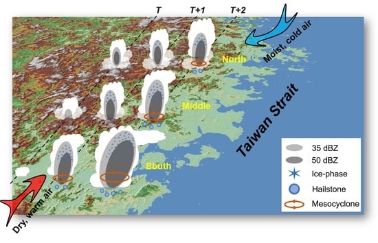
Convection appeared in succession from the north to south zones from a more clear-sky condition. The lower relative humidity, higher LFC, and larger CIN of the south might have made convective initiation harder. A southwestward-moving shear line could also have facilitated the convective initiation in the north and middle zones by interacting with high terrains. The initial convection was dominated by warm-rain processes in the north and middle zones, whereas it had a greater ice-phase component in the south zone.
(2)
The subsequent convection after onset underwent more vigorous vertical growth and horizontal expansion from the north to south zones with larger CAPE and vertical wind shear. It took a longer time to prepare the transition from shallow to deep convection in the north and middle zones. By contrast, the convective development in the south zone was explosive, which rapidly led to extremely deep convective storms with an echo top up to 18 km and evident horizontal anvil expansion.
(3)
The typical signatures in severe convection, including the weak-echo region (identified via a new-defined quantity in this study) and mesocyclone, were more pronounced from the north to south zones. This implies a higher risk of severe convective weather in the south zone where the maximum mesocyclone strength was larger than that in most giant hail cases across the contiguous U.S. Intensive hail reports were reported in the south zone.
These inter-zone differences demonstrated the strong linkage between early-stage convective development and the occurrence likelihood of severe convection and associated weather, such as supercells and hailstones, in this convection outbreak event. It is envisioned that the results presented here will help better understand the complexity of convective development from an observational perspective and benefit fine-scale convective nowcasting, especially for the southeast coast China with a subtropical climate regime.

Author Contributions

Conceptualization, Y.H. and M.Z.; methodology, Y.H., M.Z. and B.J.-D.J.; software, H.Z. and C.L.; validation, Y.H., H.Z. and D.C.; formal analysis, Y.H., M.Z. and Y.Z.; investigation, Y.H., C.L. and D.C.; resources, Y.H., M.Z. and Y.Z.; data curation, Y.H., C.L. and D.C.; writing—original draft preparation, Y.H. and M.Z.; writing—review and editing, Y.Z. and B.J.-D.J.; visualization, Y.H., M.Z. and H.Z.; supervision, Y.Z. and B.J.-D.J.; project administration, Y.H. and M.Z.; funding acquisition, Y.H. and Y.Z. All authors have read and agreed to the published version of the manuscript.

Funding

This study was funded by the National Natural Science Foundation of China (grant 41905049), the Xiamen Science and Technology Program (grant 3502Z20206079), the Open Program of LASG, Institute of Atmospheric Physics, Chinese Academy of Sciences (grant 20210625), the China Postdoctoral Science Foundation (grant 2021M702725), and the National Natural Science Foundation of China (grant 41805028).

Institutional Review Board Statement

Not applicable.

Informed Consent Statement

Not applicable.

Data Availability Statement

Not applicable.

Acknowledgments

The radar, surface, and radiosonde data, as well as the hail reports, were provided by the Fujian Meteorological Bureau. The Himawari-8 data were downloaded from the P-Tree system of the Japan Aerospace Exploration Agency (JAXA) at https://www.eorc.jaxa.jp/ptree/index.html (accessed on 13 May 2021). The ERA5 reanalysis data were provided by ECMWF and downloaded from Copernicus Climate Change Service Climate Data Store (https://cds.climate.copernicus.eu/, accessed on 20 July 2021). We thank three anonymous reviewers for their constructive comments.

Conflicts of Interest

The authors declare no conflict of interest.

References

  1. Doswell, C.A. The distinction between large-scale and mesoscale contribution to severe convection: A case study example. Weather. Forecast. 1987, 2, 3–16. [Google Scholar] [CrossRef] [Green Version]
  2. Brooks, H.E.; Doswell III, C.A.; Zhang, X.; Chernokulsky, A.M.A.; Tochimoto, E.; Hanstrum, B.; de Lima Nascimento, E.; Sills, D.M.L.; Antonescu, B.; Barrett, B. A century of progress in severe convective storm research and forecasting. Meteorol. Monogr. 2019, 59, 18.11–18.41. [Google Scholar] [CrossRef]
  3. Markowski, P.; Richardson, Y. Convection initiation. In Mesoscale Meteorology in Midlatitudes; John Wiley & Sons, Ltd.: Hoboken, NJ, USA, 2010; pp. 183–199. [Google Scholar]
  4. Weckwerth, T.M.; Parsons, D.B. A review of convection initiation and motivation for IHOP_2002. Mon. Weather. Rev. 2006, 134, 5–22. [Google Scholar] [CrossRef]
  5. Cintineo, J.L.; Pavolonis, M.J.; Sieglaff, J.M.; Heidinger, A.K. Evolution of severe and nonsevere convection inferred from GOES-derived cloud properties. J. Appl. Meteorol. Climatol. 2013, 52, 2009–2023. [Google Scholar] [CrossRef]
  6. Mecikalski, J.R.; Bedka, K.M. Forecasting convective initiation by monitoring the evolution of moving cumulus in daytime GOES imagery. Mon. Weather. Rev. 2006, 134, 49–78. [Google Scholar] [CrossRef] [Green Version]
  7. Huang, Y.; Meng, Z.; Li, W.; Bai, L.; Meng, X. General features of radar-observed boundary layer convergence lines and their associated convection over a sharp vegetation-contrast area. Geophys. Res. Lett. 2019, 46, 2865–2873. [Google Scholar] [CrossRef]
  8. Fabry, F.; Meunier, V.; Treserras, B.P.; Cournoyer, A.; Nelson, B. On the climatological use of radar data mosaics: Possibilities and challenges. Bull. Am. Meteorol. Soc. 2017, 98, 2135–2148. [Google Scholar] [CrossRef] [Green Version]
  9. Wu, C.; Liu, L.; Liu, X.; Li, G.; Chen, C. Advances in Chinese dual-polarization and phased-array weather radars: Observational analysis of a supercell in Southern China. J. Atmos. Ocean. Technol. 2018, 35, 1785–1806. [Google Scholar] [CrossRef]
  10. Meng, Z.; Yao, D.; Bai, L.; Zheng, Y.; Xue, M.; Zhang, X.; Zhao, K.; Tian, F.; Wang, M. Wind estimation around the shipwreck of Oriental Star based on field damage surveys and radar observations. Sci. Bull. 2016, 61, 330–337. [Google Scholar] [CrossRef] [Green Version]
  11. Melnikov, V.M.; Doviak, R.J. Turbulence and wind shear in layers of large doppler spectrum width in stratiform precipitation. J. Atmos. Ocean. Technol. 2009, 26, 430–443. [Google Scholar] [CrossRef]
  12. Amburn, S.A.; Wolf, P.L. VIL density as a hail indicator. Weather. Forecast. 1997, 12, 473–478. [Google Scholar] [CrossRef] [Green Version]
  13. Lemon, L.R. The radar “three-body scatter spike”: An operational large-hail signature. Weather. Forecast. 1998, 13, 327–340. [Google Scholar] [CrossRef]
  14. Meng, Z.; Bai, L.; Zhang, M.; Wu, Z.; Li, Z.; Pu, M.; Zheng, Y.; Wang, X.; Yao, D.; Xue, M.; et al. The deadliest tornado (EF4) in the past 40 years in China. Weather. Forecast. 2018, 33, 693–713. [Google Scholar] [CrossRef]
  15. Roberts, R.D.; Rutledge, S. Nowcasting storm initiation and growth using GOES-8 and WSR-88D Data. Weather. Forecast. 2003, 18, 562–584. [Google Scholar] [CrossRef] [Green Version]
  16. Mecikalski, J.R.; MacKenzie, W.M.; Koenig, M.; Muller, S. Cloud-top properties of growing cumulus prior to convective initiation as measured by meteosat second generation. Part I: Infrared fields. J. Appl. Meteorol. Climatol. 2010, 49, 521–534. [Google Scholar] [CrossRef]
  17. Mecikalski, J.R.; MacKenzie, W.M.; König, M.; Muller, S. Cloud-top properties of growing cumulus prior to convective initiation as measured by meteosat second generation. Part II: Use of visible reflectance. J. Appl. Meteorol. Climatol. 2010, 49, 2544–2558. [Google Scholar] [CrossRef] [Green Version]
  18. Walker, J.R.; MacKenzie, W.M.; Mecikalski, J.R.; Jewett, C.P. An enhanced geostationary satellite–based convective initiation algorithm for 0–2-h nowcasting with object tracking. J. Appl. Meteorol. Climatol. 2012, 51, 1931–1949. [Google Scholar] [CrossRef]
  19. Zhuge, X.; Zou, X. Summertime convective initiation nowcasting over southeastern china based on advanced himawari imager observations. J. Meteorol. Soc. Jpn. Ser. II 2018, 96, 337–353. [Google Scholar] [CrossRef] [Green Version]
  20. Sun, F.; Qin, D.; Min, M.; Li, B.; Wang, F. Convective initiation nowcasting over china from fengyun-4A measurements based on TV-L1 optical flow and BP_Adaboost neural network algorithms. IEEE J. Sel. Top. Appl. Earth Obs. Remote Sens. 2019, 12, 4284–4296. [Google Scholar] [CrossRef]
  21. Senf, F.; Dietzsch, F.; Hünerbein, A.; Deneke, H. Characterization of initiation and growth of selected severe convective storms over central europe with MSG-SEVIRI. J. Appl. Meteorol. Climatol. 2015, 54, 207–224. [Google Scholar] [CrossRef]
  22. Senf, F.; Deneke, H. Satellite-based characterization of convective growth and glaciation and its relationship to precipitation formation over Central Europe. J. Appl. Meteorol. Climatol. 2017, 56, 1827–1845. [Google Scholar] [CrossRef]
  23. Mecikalski, J.R.; Rosenfeld, D.; Manzato, A. Evaluation of geostationary satellite observations and the development of a 1–2 h prediction model for future storm intensity. J. Geophys. Res. Atmos. 2016, 121, 6374–6392. [Google Scholar] [CrossRef]
  24. Mecikalski, J.R.; Li, X.; Carey, L.D.; McCaul, E.W.; Coleman, T.A. Regional comparison of GOES cloud-top properties and radar characteristics in advance of first-flash lightning initiation. Mon. Weather. Rev. 2013, 141, 55–74. [Google Scholar] [CrossRef] [Green Version]
  25. Chen, M.; Wang, Y.; Gao, F.; Xiao, X. Diurnal evolution and distribution of warm-season convective storms in different prevailing wind regimes over contiguous North China. J. Geophys. Res. Atmos. 2014, 119, 2742–2763. [Google Scholar] [CrossRef]
  26. Huang, Y.; Meng, Z.; Li, J.; Li, W.; Bai, L.; Zhang, M.; Wang, X. Distribution and variability of satellite-derived signals of isolated convection initiation events over Central Eastern China. J. Geophys. Res. Atmos. 2017, 122, 11–357. [Google Scholar] [CrossRef]
  27. Luo, Y.; Wang, H.; Zhang, R.; Qian, W.; Luo, Z. Comparison of rainfall characteristics and convective properties of monsoon precipitation systems over South China and the Yangtze and Huai river basin. J. Clim. 2013, 26, 110–132. [Google Scholar] [CrossRef] [Green Version]
  28. Xu, W. Precipitation and convective characteristics of summer deep convection over East Asia observed by TRMM. Mon. Weather. Rev. 2013, 141, 1577–1592. [Google Scholar] [CrossRef]
  29. Houze, R.A., Jr.; Rasmussen, K.L.; Zuluaga, M.D.; Brodzik, S.R. The variable nature of convection in the tropics and subtropics: A legacy of 16 years of the tropical rainfall measuring mission satellite. Rev. Geophys. 2015, 53, 994–1021. [Google Scholar] [CrossRef] [PubMed]
  30. Zuluaga, M.D.; Houze, R.A. Extreme convection of the near-equatorial Americas, Africa, and adjoining oceans as seen by TRMM. Mon. Weather. Rev. 2015, 143, 298–316. [Google Scholar] [CrossRef] [Green Version]
  31. Zhou, X.; Huang, G.; Baetz, B.W.; Wang, X.; Cheng, G. PRECIS—projected increases in temperature and precipitation over Canada. Q. J. R. Meteorol. Soc. 2018, 144, 588–603. [Google Scholar] [CrossRef]
  32. Zhou, X.; Huang, G.; Li, Y.; Lin, Q.; Yan, D.; He, X. Dynamical downscaling of temperature variations over the canadian prairie provinces under climate change. Remote Sens. 2021, 13, 4350. [Google Scholar] [CrossRef]
  33. Zhou, X.; Huang, G.; Piwowar, J.; Fan, Y.; Wang, X.; Li, Z.; Cheng, G. Hydrologic impacts of ensemble-RCM-projected climate changes in the Athabasca River basin, Canada. J. Hydrometeorol. 2018, 19, 1953–1971. [Google Scholar] [CrossRef] [Green Version]
  34. Zhou, X.; Huang, G.; Wang, X.; Cheng, G. Future changes in precipitation extremes over Canada: Driving factors and inherent mechanism. J. Geophys. Res. Atmos. 2018, 123, 5783–5803. [Google Scholar] [CrossRef]
  35. Xia, R.; Zhang, D.-L.; Wang, B. A 6-yr cloud-to-ground lightning climatology and its relationship to rainfall over central and Eastern China. J. Appl. Meteorol. Climatol. 2015, 54, 2443–2460. [Google Scholar] [CrossRef]
  36. Yang, X.; Li, Z. Increases in thunderstorm activity and relationships with air pollution in southeast China. J. Geophys. Res. Atmos. 2014, 119, 1835–1844. [Google Scholar] [CrossRef]
  37. Wang, H.; Luo, Y.; Jou, B.J.-D. Initiation, maintenance, and properties of convection in an extreme rainfall event during SCMREX: Observational analysis. J. Geophys. Res. Atmos. 2014, 119, 13206–13232. [Google Scholar] [CrossRef]
  38. Li, M.; Luo, Y.; Zhang, D.L.; Chen, M.; Wu, C.; Yin, J.; Ma, R. Analysis of a record-breaking rainfall event associated with a monsoon coastal megacity of south china using multisource data. IEEE Trans. Geosci. Remote Sens. 2021, 59, 6404–6414. [Google Scholar] [CrossRef]
  39. Ribeiro, B.Z.; Machado, L.A.T.; Huamán Ch., J. H.; Biscaro, T.S.; Freitas, E.D.; Mozer, K.W.; Goodman, S.J. An evaluation of the GOES-16 rapid scan for nowcasting in Southeastern Brazil: Analysis of a severe hailstorm case. Weather. Forecast. 2019, 34, 1829–1848. [Google Scholar] [CrossRef]
  40. Bessho, K.; Date, K.; Hayashi, M.; Ikeda, A.; Imai, T.; Inoue, H.; Kumagai, Y.; Miyakawa, T.; Murata, H.; Ohno, T.; et al. An introduction to Himawari-8/9—Japan’s New-generation geostationary meteorological satellites. J. Meteorol. Soc. Japan. Ser. II 2016, 94, 151–183. [Google Scholar] [CrossRef] [Green Version]
  41. Matthee, R.; Mecikalski, J.R.; Carey, L.D.; Bitzer, P.M. Quantitative differences between lightning and nonlightning convective rainfall events as observed with polarimetric radar and MSG satellite data. Mon. Weather. Rev. 2014, 142, 3651–3665. [Google Scholar] [CrossRef]
  42. Zhao, K.; Wang, M.; Xue, M.; Fu, P.; Yang, Z.; Chen, X.; Zhang, Y.; Lee, W.-C.; Zhang, F.; Lin, Q.; et al. Doppler radar analysis of a tornadic miniature supercell during the landfall of typhoon mujigae (2015) in South China. Bull. Am. Meteorol. Soc. 2017, 98, 1821–1831. [Google Scholar] [CrossRef] [Green Version]
  43. Lensky, I.M.; Rosenfeld, D. Clouds-aerosols-precipitation satellite analysis tool (CAPSAT). Atmos. Chem. Phys. 2008, 8, 6739–6753. [Google Scholar] [CrossRef] [Green Version]
  44. Hersbach, H.; Bell, B.; Berrisford, P.; Hirahara, S.; Horányi, A.; Muñoz-Sabater, J.; Nicolas, J.; Peubey, C.; Radu, R.; Schepers, D.; et al. The ERA5 global reanalysis. Q. J. R. Meteorol. Soc. 2020, 146, 1999–2049. [Google Scholar] [CrossRef]
  45. Amante, C.; Eakins, B.W. ETOPO1 1 Arc-minute global relief model: Procedures, data sources and analysis. NOAA Tech. Memo. NESDIS NGDC-24 2009, 10, V5C8276M. [Google Scholar] [CrossRef]
  46. Cressman, G.P. An operational objective analysis system. Mon. Weather. Rev. 1959, 87, 367–374. [Google Scholar] [CrossRef]
  47. Zipser, E.J.; Lutz, K.R. The vertical profile of radar reflectivity of convective cells: A strong indicator of storm intensity and lightning probability? Mon. Weather. Rev. 1994, 122, 1751–1759. [Google Scholar] [CrossRef] [Green Version]
  48. Witt, A.; Eilts, M.D.; Stumpf, G.J.; Johnson, J.T.; Mitchell, E.D.W.; Thomas, K.W. An enhanced hail detection algorithm for the WSR-88D. Weather. Forecast. 1998, 13, 286–303. [Google Scholar] [CrossRef] [Green Version]
  49. Brimelow, J.C.; Reuter, G.W.; Bellon, A.; Hudak, D. A radar-based methodology for preparing a severe thunderstorm climatology in central Alberta. Atmos.-Ocean. 2004, 42, 13–22. [Google Scholar] [CrossRef] [Green Version]
  50. Lee, R.R.; White, A. Improvement of the WSR-88D mesocyclone algorithm. Weather. Forecast. 1998, 13, 341–351. [Google Scholar] [CrossRef]
  51. Andra, D.L. The origin and evolution of the WSR-88D mesocyclone recognition nomogram. In Proceedings of the 28th Conference Radar Meteorology, Austin, TX, USA, 7–12 September 1997; pp. 364–365. [Google Scholar]
  52. Blair, S.F.; Deroche, D.R.; Boustead, J.M.; Leighton, J.W.; Barjenbruch, B.L.; Gargan, W.P. A radar-based assessment of the detectability of giant hail. E-J. Sev. Storms Meteorol. 2011, 6, 1–30. [Google Scholar]
  53. Smith, B.T.; Thompson, R.L.; Dean, A.R.; Marsh, P.T. Diagnosing the conditional probability of tornado damage rating using environmental and radar attributes. Weather. Forecast. 2015, 30, 914–932. [Google Scholar] [CrossRef]
  54. Hartung, D.C.; Sieglaff, J.M.; Cronce, L.M.; Feltz, W.F. An intercomparison of UW cloud-top cooling rates with WSR-88D radar data. Weather. Forecast. 2013, 28, 463–480. [Google Scholar] [CrossRef]
  55. Matthee, R.; Mecikalski, J.R. Geostationary infrared methods for detecting lightning-producing cumulonimbus clouds. J. Geophys. Res. Atmos. 2013, 118, 6580–6592. [Google Scholar] [CrossRef]
  56. Hong, G.; Yang, P.; Heidinger, A.K.; Pavolonis, M.J.; Baum, B.A.; Platnick, S.E. Detecting opaque and nonopaque tropical upper tropospheric ice clouds: A trispectral technique based on the MODIS 8–12 μm window bands. J. Geophys. Res. 2010, 115. [Google Scholar] [CrossRef]
  57. Yuan, J.; Houze, R.A. Global variability of mesoscale convective system anvil structure from A-train satellite data. J. Clim. 2010, 23, 5864–5888. [Google Scholar] [CrossRef]
  58. Pilewskie, P.; Twomey, S. Cloud phase discrimination by reflectance measurements near 1.6 and 2.2 μm. J. Atmos. Sci. 1987, 44, 3419–3420. [Google Scholar] [CrossRef] [Green Version]
  59. Baum, B.A.; Soulen, P.F.; Strabala, K.I.; King, M.D.; Ackerman, S.A.; Menzel, W.P.; Yang, P. Remote sensing of cloud properties using MODIS airborne simulator imagery during SUCCESS: 2. Cloud thermodynamic phase. J. Geophys. Res. Atmos. 2000, 105, 11781–11792. [Google Scholar] [CrossRef]
  60. Lindsey, D.T.; Hillger, D.W.; Grasso, L.; Knaff, J.A.; Dostalek, J.F. GOES climatology and analysis of thunderstorms with enhanced 3.9-μm reflectivity. Mon. Weather. Rev. 2006, 134, 2342–2353. [Google Scholar] [CrossRef] [Green Version]
  61. Du, Y.; Chen, G.; Han, B.; Bai, L.; Li, M. Convection initiation and growth at the coast of South China. Part II: Effects of the terrain, coastline, and cold pools. Mon. Weather. Rev. 2020, 148, 3871–3892. [Google Scholar] [CrossRef]
  62. Williams, E.R.; Weber, M.E.; Orville, R.E. The relationship between lightning type and convective state of thunderclouds. J. Geophys. Res. Atmos. 1989, 94, 13213–13220. [Google Scholar] [CrossRef] [Green Version]
Figure 1. (a) Topography map of Southeastern China with the locations of operational radars (black squares; including Fuzhou (FZ), Quanzhou (QZ), Xiamen (XM), Zhangzhou (ZZ), and Longyan (LY) radars) and radiosondes (red triangles; including Fuzhou (FZ) and Xiamen (XM) radiosondes) used in the study. (b) Occurrence frequencies of convection (≥35 dBZ echoes; shaded) and strong convection (≥50 dBZ echoes; only the 15% frequency is shown by the red contour) during 1200–1500 LST on 6 May 2020 with hail reports (blue triangles) and in situ maximum hourly rainfall (circles). The three convection-active zones analyzed in this study are indicated by black and magenta boxes in (a) and (b), respectively. The 230 km detection range for each radar is shown by the gray rings in (a). The occurrence frequency in (b) was calculated based on maximum reflectivity images for every 0.01° × 0.01° grid, and it was normalized by the total image number during 1200–1500 LST. The topographic elevations of 500, 800, and 1000 m are contoured as blue lines (from dark to light) in (b).
Remotesensing 14 00131 g001
Figure 2. Methodological framework for two remote sensing datasets used in this study.
Remotesensing 14 00131 g002
Figure 6. Maximum radar reflectivity images with in situ 5 min rainfall (black dots) at (a) 1230, (b) 1300, (c) 1336, and (d) 1418 LST on 6 May 2020. Three convection-active zones are indicated by the black boxes.
Remotesensing 14 00131 g006
Figure 7. Time–height diagrams of (a1c1) the convection (≥35 dBZ echoes) frequency, (a2c2) the strong convective precipitation (≥50 dBZ echoes) frequency with in situ 5 min rainfall (colored dots), and (a3c3) the maximum reflectivity for three convection-active zones (north: a1a3; middle: b1b3; south: c1c3) during 1200–1500 LST on 6 May 2020. The time interval is 6 min, and the height interval is 0.5 km. For each time interval, the frequencies in (a1c1) and (a2c2) were normalized by the total radar-detected echo number at each vertical interval and are presented as a fraction. The horizontal dashed lines indicate the freezing and −20 °C levels. The slant dashed lines in (c1c3) indicate the echo top slopes between 1248 and 1412 LST. The black triangles represent the convective initiation times.
Remotesensing 14 00131 g007
Figure 8. Contoured frequency by altitude diagrams (CFADs) for the three convection-active zones (north: a1a4; middle: b1b4; south: c1c4) at the four representative times in Figure 6. The black and gray curves, respectively, show the profiles of mean and maximum reflectivity. The black dashed lines indicate the freezing and −20 °C levels. The gray dashed lines indicate 35 dBZ. The reflectivity width is 5 dBZ, and the vertical interval is 0.5 km. The frequencies were normalized by the total radar-detected echo number at each vertical interval and are presented as fractions. Note that values below 0 dBZ are involved here, but their frequencies are not shown.
Remotesensing 14 00131 g008
Figure 9. Example of vertically integrated liquid water content (VIL) and its derivations: (a) VIL (shading) image at 1336 LST; (b) vertical cross-section of the mosaicked reflectivity from the multiple radars in Figure 1a along the line segment (blue) in (a); (c) VIL (blue solid line) and its density (blue dashed line), as well as the ratios of VIL above the freezing (red solid line) and −20 °C (red dashed line) levels corresponding to the vertical cross-section in (b). The black boxes in (a) indicate three convection-active zones. The areas with a VIL ratio above the freezing level of more than 75% are shown as black contour lines in (a). The VIL-weighted equivalent altitude is indicated by the solid line in (b). The dashed lines in (b) indicate the freezing and −20 °C levels. The defined weak-echo region is represented by the dashed box in (b,c).
Remotesensing 14 00131 g009
Figure 10. Temporal variations in the (a) vertically integrated liquid water content (VIL), (b) VIL density, and (c) weak-echo region (WER) for three convection-active zones (S, south; M, middle; N, north). Here, the WER is defined as the region with a VIL over 20 kg m−2 and a VIL ratio above the freezing level of more than 75%.
Remotesensing 14 00131 g010
Figure 12. Temporal variations in the frequency distributions of Himawari-8-based (ac) 10.4 μm brightness temperature (BT) and (df) BT difference (BTD) between 6.2 and 7.3 μm to describe cloud-top height in three convection-active zones. The frequency of the BT/BTD interval at each 10 min scan was normalized by the total BT/BTD number and presented as a fraction. The dashed lines from top to bottom represent the upper limit values, upper quartiles, medians, lower quartiles, and lower limit values at a time for all pixels within a zone, and the diamond symbols represent the mean values. The fraction distributions of cloudy pixels after the cloud mask are shaded. The blue triangles in (ac) represent the first remarkable cooling rate of ≥5 °C (10 min)−1 in minimum BT field. The red labels in (b) show the equivalent altitudes of some key temperature levels. Note that the vertical axis is reversed in (ac).
Remotesensing 14 00131 g012
Figure 13. Images of Himawari-8 interest fields analyzed in this study at (a1f1) 1200, (a2f2) 1320, and (a3f3) 1350 LST, including the (a1a3) 10.4 μm brightness temperature (BT), (b1b3) BT difference (BTD) between 6.2 and 7.3 μm, (c1c3) 0.47 μm reflectance (ρ), (d1d3) BTD between 12.4 and 10.4 μm, (e1e3) trispectral difference, and (f1f3) 3.9 μm ρ. Three convection-active zones are indicated by the black boxes.
Remotesensing 14 00131 g013
Figure 14. As in Figure 12 but for the (ac) 0.47 μm reflectance (ρ) and (df) brightness temperature difference (BTD) between 12.4 and 10.4 μm to describe cloud optical thickness.
Remotesensing 14 00131 g014
Figure 15. As in Figure 12 but for the (ac) trispectral difference to describe cloud-top glaciation and (df) 3.9 μm reflectance (ρ) to describe cloud-top glaciation and particle size. Note that the vertical axis is reversed in (df). The blue triangles in (ac) represent the first times when the fractions of cloudy pixels with positive values were larger than 1%.
Remotesensing 14 00131 g015
Figure 16. Temporal collocations between hail occurrence (indicated by the TBSS signature; black dots) and 14 radar- or satellite-derived signatures (shown on the right-hand side) for three convection-active zones (north, middle, and south—from the top to bottom rows in each subset). See text for more interpretation.
Remotesensing 14 00131 g016
Publisher’s Note: MDPI stays neutral with regard to jurisdictional claims in published maps and institutional affiliations.

