Article

Integrated Mapping of Spatial Urban Dynamics—A European-Chinese Exploration. Part 1—Methodology for Automatic Land Cover Classification Tailored towards Spatial Allocation of Ecosystem Services Features

1
UFZ-Helmholtz Centre for Environmental Research, Department Urban and Environmental Sociology, Permoserstr. 15, 04318 Leipzig, Germany
2
Ministry of Education Key Laboratory for Biodiversity Science and Ecological Engineering, National Observations and Research Station for Wetland Ecosystems of the Yangtze Estuary, Shanghai Institute of EcoChongming (SIEC), Fudan University, Shanghai 200433, China
3
Ministry of Education Key Laboratory for Earth System Modelling, Department of Earth System Science, Tsinghua University, Beijing 100084, China
*
Author to whom correspondence should be addressed.
Remote Sens. 2021, 13(9), 1744; https://doi.org/10.3390/rs13091744
Submission received: 10 February 2021 / Revised: 22 April 2021 / Accepted: 25 April 2021 / Published: 30 April 2021
(This article belongs to the Special Issue Understanding Urban Systems Using Remote Sensing)

Abstract

:
Urbanisation processes inherently influence land cover (LC) and have dramatic impacts on the amount, distribution and quality of vegetation cover. The latter are the source of ecosystem services (ES) on which humans depend. However, the temporal and thematical dimensions are not documented in a comparable manner across Europe and China. Three cities in China and three cities in Europe were selected as case study areas to gain a picture of spatial urban dynamics at intercontinental scale. First, we analysed available global and continental thematic LC products as a data pool for sample selection and referencing our own mapping model. With the help of the Google Earth Engine (GEE) platform and earth observation data, an automatic LC mapping method tailored for more detailed ES features was proposed. To do so, differentiated LC categories were quantified. In order to obtain a balance between efficiency and high classification accuracy, we developed an optimal classification model by evaluating the importance of a large number of spectral, texture-based indices and topographical information. The overall classification accuracies range between 73% and 95% for different time slots and cities. To capture ES related LC categories in great detail, deciduous and coniferous forests, cropland, grassland and bare land were effectively identified. To understand inner urban options for potential new ES, dense and dispersed built-up areas were differentiated with good results. In addition, this study focuses on the differences in the characteristics of urban expansion witnessed in China and Europe. Our results reveal that urbanisation has been more intense in the three Chinese cities than in the three European cities, with an 84% increase in the entire built-up area over the last two decades. However, our results also show the results of China’s ecological restoration policies, with a total of 963 km2 of new green and blue LC created in the last two decades. We proved that our automatic mapping can be effectively applied to future studies, and the monitoring results will be useful for consecutive ES analyses aimed at achieving more environmentally friendly cities.

Graphical Abstract

1. Introduction

1.1. Impact of Urbanisation Processes on Ecosystem Services

Increased urbanisation and the expansion of urban areas cause radical changes to and the eradication and fragmentation of ecosystems and green infrastructure—particularly in China but also in Europe. Europe is already one of the most urbanised continents in the world with about 74% of Europeans living in urban areas, while the level of urbanisation in Asia is around 50% [1]. The urbanisation trend continues in Europe: Projections expect 84% of the total population to be living in urban areas by 2050, while China’s urbanisation rate is expected to grow from the present day’s 61% to 80% by 2050 (ibid).
The challenges that cities face today include inequality at various levels, such as inequality of resources and ecosystem service (ES) provision, as well as environmental harm caused by increasing pressure by land takeover [2,3]. Since intense interdependencies exist regarding the use of resources, urban growth has a tremendous impact on resource regimes and ecosystems which make urban dwellers simultaneously culprits and victims of urbanisation processes [4]. It is for this reason that the United Nations Sustainable Development Goals (SDG), especially SDG 11 “Make cities inclusive, safe, resilient and sustainable” [5] demand interactions in cities and understand the great potential with which cities can contribute to sustainable development.
Urbanisation may be a global phenomenon. Yet, it does not play out as a homogeneous process across continents and countries. Its primary driver is population growth, its physical expression and the patterns are manifold, as is its impact on the urban environment. To understand both urban impacts on local or regional ecosystems and urban dependence on ecosystems, it is essential to map the variation within and between cities. Urban land expands in different directions to provide space for living, public infrastructure, and business at quite distinct urban land expansion rates, thus shifting its physical boundaries into the more natural hinterland, which again diminishes non-artificial LC in these peri-urban areas.
By mapping urbanisation processes over time, the different development phases of cities in Europe and China become transparent. Such spatial investigations can explain not only their growth patterns, like densification processes or leap-frog development, but also the specific velocity and direction of change. Analysing urbanisation processes reveals which other LC types have been superseded by buildings and urban infrastructures, at which pace and in which magnitude the loss has taken place.

1.2. Transferable Land Cover Mapping Approach Based on Remote Sensing

1.2.1. Ready-Made Remote Sensing (RS) Products

When capturing the urban footprint, one of the most appropriate tools to use is RS, its images and its methods [6]. Satellite images are the best source for mapping land surface over large areas as well as over long periods of time. Observations need to be extensive, regular and consistent to establish baselines and trends. It is a spatial analytical technology that meets various scientific and planning requirements. The physical structure and composition of urban areas can be mapped and monitored using the various spatial and temporal scales at which images are acquired by different sensor systems. Landsat is the longest-running civilian Earth-observing programme and fundamentally serves environmental observation. Based on its vast datasets, global data infrastructures have been developed to generate and disseminate mapping products that are made available through different agencies (NASA; ESA; CNSA; JAXA; ISRO; AEB). Some of these mapping products, like the Global Human Settlement Layer (GHSL), are available at global scale and increase knowledge for organisations such as the UN, the OECD and the World Bank, to name a few. They help researchers understand the global dynamics in urbanisation processes and specialise in mapping built-up surfaces at an aggregated scale [7]. China made the first open-access, high-resolution map of Earth’s land cover available to the United Nations, the GlobeLand30, as a contribution towards global sustainable development and climate change mitigation [8]. Annual maps of global urbanisation processes have been developed since 1985, such as the GAIA (global artificial impervious area; [9]) and GAUD (global annual urban dynamics; [10]) datasets. Yet, there is more detailed spatial information for continents like Europe, where there are long-time projects such as the CORINE (Coordination of Information on the Environment) Land Cover (initiated in the mid-1980s), the Urban Atlas (initiated in 2006, with updates in 2012 and 2018) and the Copernicus services. The latter launched its Land Monitoring Service in 2012, and all these platforms provide data on the European environment and various detailed information to users free of charge. So, what we know and what we have at hand are a multitude of publicly accessible products for environmental research containing defined sets of LC categories at defined scales over specific periods of time or time slots. Such readily available spatial information is especially of value for intra- and international comparisons in spatial planning and research tackling urban and regional environmental issues. What is lacking is a standardised set of LC categories across all these systems. They hardly cover similar time spans, and most neither differentiate between dense and dispersed urban fabric, nor between different types of vegetation cover (for details see Table 1). This deficiency may be caused by the specifications under which they were developed, or by the specific scale they refer to. For this reason, these thematic products can be used for general comparisons and as a profound basis for further in-depth analysis.

1.2.2. Further RS Requirements for Capturing Key Elements of Urban LC Categories across Continents

To assess LC in cities around the globe, all spatial information must be provided at the same spatial and temporal scale and with the same detailed categories. If the designs of the above-mentioned publicly available RS catalogues do not meet the requirements for research on LC related to urban ES, then those catalogues can be taken as basic input for training and validation to establish an ambitious classification scheme. Enhanced accuracy would make RS more suitable for monitoring biodiversity loss and ecosystem dynamics, for example, and for other applications that depend on baseline and changing LC [11]. To improve the accuracy of products derived from shared satellite observations of urban areas, a spatial analysis needs to be undertaken developing elaborated methods and tools. When mapping LC elements to determine the extent and condition of natural capital and its biophysical expression over time, then the Google Earth Engine (GEE) serves as an effective analytical platform. GEE is a sophisticated and scalable mapping tool, with which we are enabled to determine the time courses of urban growth rates and quantify the other more natural LC types that are being lost through advancing urbanisation.
The aim of this study is to design an automatic classification method at the intercontinental scale to understand the different urbanisation processes in Europe and China, firstly by exploiting global urban datasets and secondly by a distinct mapping of grey, green and blue features as a basis for further ES analysis. The methodological innovation of our contribution includes an automatic variable selection for a more efficient creation and application of the classification model. To realise this, a well-developed workflow for an automatic samples collection based on the above-mentioned multi-source ground truth and raster-based land cover products is presented. It is a prerequisite to collect spatial information for both continents to obtain training and validation data. For reasons of consistent results, we aim to capture key categories by elaborating a novel classification approach. To make our approach easily reproducible for other cities, we develop this processing workflow based on GEE. This enables us to take into account the existing thematic products for LC, and extract valuable information for our discerning, globally applicable mapping model presented here in Part 1. Because we will perform further ES analyses in urban areas (Part 2), we undertake the effort to differentiate various types of vegetation with distinctions between grassland and cropland, and deciduous and coniferous forests. Up to present, there are no existing products for both China and Europe over decades showing such levels of detail. For this reason, our research tackles this central question: Can we capture a detailed LC mapping that contains highly differentiated categories for selected cities in Asia and Europe by developing a streamlined processing in GEE? This encompasses two secondary questions: Can we make distinctions between deciduous and coniferous forests and between dense and dispersed urban areas? To what extent can we map cropland, grassland, and bare land for each city?

2. Approach

2.1. Satellite Images and Ancillary Data

All data from the Landsat series are available at the GEE platform. In this research, we used various datasets from Landsat sensors including the Landsat 5 Thematic Mapper (TM) for 2000 and 2010, and the Landsat 8 Operational Land Imager (OLI)/Thermal Infrared Sensor (TIRS) for 2020. The Landsat series offer the most long-term satellite images at the same spatial scale of 30 m ground resolution and make it possible to extract the same spectral resolution over decades. Their global repetition rate of 16 days means that data is acquired throughout the entire year which makes it easier to find images with no or minimum cloud cover.

2.2. Reference Data for Sample Points

The selection of reference data was driven by two main factors. On the one hand, spatial coverage was important, as the different urban areas are located across China and Europe. Thus, only global datasets were considered at the beginning. This selection proved to be too narrow, so we expanded our analysis to include European and Chinese datasets. They feature different LC classes in greater detail. The second factor we considered pertains to the temporal coverage, which represents continuity. All the selected thematic mapping products feature different intervals, but they are available for at least three points in time and thereby map the changes in LC over decades. The data used to generate the sample points in this study were sourced from the following ground-truth-based and remotely sensed products.

2.2.1. Datasets for Sample Point Extraction Based on Ground Truth

CORINE Land Cover

The Coordination of Information on the Environment land cover, also known as the CORINE Land Cover or CLC, is a European land use and land cover product spanning the years 1990 to currently 2018 in six- to 10-year increments. The classification system is based on 13 main classes and contains 44 classes in total. Its contents are generated through manual and automatic classification of satellite images as well as field surveys. The product is available as a raster dataset with a resolution of 30 m. The overall accuracy is specified as 87% with different classes ranging from 70% to 95%, but several studies have shown this to be inaccurate and, depending on the land cover and land use class, the rate of accuracy ranges from 82.8% to 97.6% for different years [12,13,14]. However, given its good temporal coverage, the product was deemed to be a suitable reference for this study.

Urban Atlas

The Urban Atlas is another European mixed land cover and land use product. It is available for the years 2006, 2012 and 2018 with 21 and 27 classes for the last two versions. The coverage was also increased from 305 to 695 cities in 2012 and then to 788 cities in 2018 [15,16]. Spatial accuracy is presented at 5 m [16]. The accuracy is reported to be above 80% for all classes, whereby the 2012 product has different accuracies for urban and rural areas (98.4% and 96.9% respectively) [15,17]. Agreement between the GlobeLand30 product and the Urban Atlas is reported to be above 85% [18]. The urban setting of this product along with its temporal continuity and high spatial accuracy meant that it was also considered to be a good reference.

The Land Use and Land Cover Area Frame Survey (LUCAS) Sample Points

LUCAS is a land cover and land use survey for Europe conducted by the European statistical office [19] on a three-year basis. The dataset includes some 240,000 individual points in the latest version from 2018, all measured in situ. Thus, the dataset not only provides information about the predominant LC, but also about land use. It features 16 thematic classes that are determined either through the interpretation of RS data or by on-site evaluation, along with photo documentation taken in the field. The field work guidelines allow for consistent classification by minimising the influence of the respective surveyor on site [19]. Because of their consistency, the sample points are available over time and match well with the classes used for the mapping. For this reason, they are used to validate the LC mapping of the European cities studied here.

2.2.2. Datasets for Sample Point Extraction Based on RS Products

GlobeLand30

GlobeLand30 is a 30-m resolution global LC data product for 2000, 2010 and 2020 that was developed by the Chinese Ministry of Natural Resources [8]. It comprises ten thematic classes including cropland, forest, grassland, shrubland, wetland, water bodies, tundra, artificial surface, bare land, perennial snow, and ice. The multispectral images used to develop and update the LC classification are derived from the sensors TM5, ETM+, OLI of Landsat (USA), as well as HJ-1 and GF-1 (China). Image selection followed the principle that the image is cloudless (or has less cloud), and the multispectral images refer to the growing season of vegetation within ± 2 years of the baseline year when the data was produced or updated. For areas that are difficult to obtain, the image acquisition time could be adapted to ensure the integrity of the global coverage. The total accuracy of GlobeLand30 was 83.5% in 2010 and 85.7% in 2020, their Kappa coefficients were 0.78 and 0.82, respectively. The results were validated by over 230,000 points from the whole dataset using the landscape index sampling model [20]. It can provide us with the latest information on LC in 2020 for validating the current mapping work.

Forest Maps

In order to further distinguish between different forest types (deciduous and coniferous) in our mapping model, the 2010 China Forest Type Classification and Mapping Products were used to select sample points for the three Chinese cities [21]. The 30 m resolution forest map for China was established using Landsat TM, by the Moderate Resolution Imaging Spectrometer (MODIS) time-series at 250 m ground resolution, by the Enhanced Vegetation Index (EVI) and other auxiliary datasets. The classification of forested areas is comprised of six types: coniferous/deciduous broadleaf, coniferous/deciduous coniferous, mixed forests, and bamboos. To assess the accuracy of the forest/non-forest classification, 2195 test sample units were used independently of the training sample. The quality indicates a producer’s accuracy (PA) of 92.0%, user’s accuracy (UA) of 95.7% and an overall accuracy (OA) of 72.7%.

The Chinese Academy of Sciences (CAS) LC Dataset

To classify the Chinese cities more efficiently with regard to the distinction of bare land, waterbodies and grassland, we used the 30 m resolution land use and land cover products derived from Resource and Environment Science Data Center, CAS (www.resdc.cn. Note: This source of land use and land cover products is not entirely public. The products with 1-km resolution are open access after free registration, while the 30-m products should be requested and purchased on the website. All information on the website is in Chinese only). Here, we extracted the maps for 2000, 2005, 2010 and 2015 that are based on multi-sources RS images from Landsat 5 TM, Landsat 7 ETM, and Landsat 8 OLI. This sequence of datasets was validated by sample points through field investigation with Kappa coefficients of more than 0.8 and accuracy of bare land, waterbodies and grassland of more than 85%, 90%, and 90% respectively [22].

The Peking University UrbanScape Essential Dataset (PKU-USED) for Beijing

To distinguish between dense and dispersed built-up areas, we made use of the USED maps to create sample points to validate our current mapping for Beijing. We extracted the dataset using the functional zones mapping tools [23,24] which are based on the Chinese satellites ZY-3, GF-6, and GEE imagery repository [25]. The urban functional zones are divided into twelve categories and have a spatial resolution of 2.4 m.

The Thematic Mapping Product GAIA

As a high-resolution global artificial impervious area product, GAIA acquired Landsat Thematic Mapper (TM), Enhanced Thematic Mapper Plus (ETM+), and Landsat 8 Operational Land Imager (OLI) data in different years to map the artificial impervious areas. It features a 30 m resolution and contains more than 30 years of records (from 1985 to 2018) with a mean overall accuracy of above 90% [9]. In this study, GAIA was used to help generate samples for built-up areas in the six cities in 2000, 2010, and 2020. The GAIA dataset can be freely downloaded from http://data.ess.tsinghua.edu.cn and is also available on GEE (Tsinghua/FROM-GLC/GAIA/v10).

2.2.3. Input Data for Samples Generation

We extracted all the thematic products at the global and continental scales to generate samples. This sample selection is essential for training the mapping model and for validation purposes. These data served as our input data source pool, out of which we extracted the best fit for our own mapping model. The details of the LC products we used are listed above, the methodology of how we used the samples selection is explained in Section 3.3.2.

3. Discerning Methodology

3.1. Study Area

The study area is composed of three cities in Europe (Paris Region, Aarhus and Velika Gorica) and three in China (Beijing, Shanghai, Ningbo). Figure 1 illustrates their locations. These urban areas vary in their spatial extent, population number and density, and the velocity of their urbanisation processes. Their diversity is valuable for testing existing mapping products at an intercontinental scale and demonstrating the applicability of our mapping model. By choosing a diverse variety of cities, we can ensure the transferability of our GEE approach. The common interest among the six cities is their commitment to foster green infrastructure and their related ES in the respective urban areas.
Paris Region is the capital region of France with a land area of 12,012 km2, home to 12 million inhabitants or 18.2% of the population of France. 21% of the territory is urbanised (16% totally impermeable), 23% covered by forests and 47% of the territory is composed of cultivated, mainly intensive open field crops. Biodiversity has greatly depleted over the last decade, which is especially visible in agricultural areas and in urban parks and gardens. Green space per inhabitant is very scarce in the four départements within the inner ring of the Paris Region—it varies between 2 and 10 m2 depending on administrative unit. The region experiences substantial land take with more than 900 hectares of rural area consumed each year by urbanisation.
City of Aarhus is the second largest city in Denmark with 273,077 inhabitants with a land area of 468 km2 and a total municipal population of 341,000. The urban area of Aarhus is 91 km2 and its population density is around 3000 inhabitants per km2, compared to an average of 272 people per km2 for the entire municipality. Over 90% of the inhabitants have access to green space within 500 m and the authorities aim to sustain or increase green area per inhabitant through green/blue structure planning despite densification. The city anticipates densification with an additional 75,000 inhabitants by 2030.
City of Velika Gorica is the sixth largest city in Croatia with 63,517 inhabitants and is located in close vicinity to the City of Zagreb, the capital of Croatia. The municipality covers 328 km2 and has 193 inhabitants per km2. In contrast, the urban area covers only around 13 km2 (ca. 4%) and experienced intensive construction during the 1970s and 1980s. Here, 32,000 inhabitants live with a population density of around 2500 people per km2. In the near vicinity, lowland, humid wooded areas host the highest woodland biodiversity nationally.
Beijing is the capital city of China with a land area of 16,410 km2. Beijing has gone through a rapid urbanisation process in the past four decades. Beijing’s permanent population increased from 13.8 million in 2000 to 21.7 million in 2016, while the built-up area expanded from 488 km2 to 1400 km2 in the same period. Urban green space accounts for about 821 km2, corresponding to 21 m2 per inhabitant. By the end of 2015 there were 339 registered municipal parks.
Shanghai is the largest city in China. It is located on the banks of the Yangtze River Delta in Eastern China and covers a total area of 6340 km2. Shanghai has the world’s largest port and a population of 24.2 million, including a transient population of more than two million. The city owns various types of natural wetlands which account for 23.5% of its total area, but these have suffered from a loss of biodiversity and vegetation decline. As the administration aims to transform the city into an “ecological city”, construction and protection of green spaces, forests, and wetlands have been launched across the city.
Ningbo is an important port city in China. Located 220 km south of Shanghai, it belongs to the densely populated Yangtze River Delta region. Having undergone heavy urbanisation processes including land reclamation that involved dams, bridges, and port constructions, it has expanded its surface area. Presently, it covers an area of 9670 km2 and is home to about 5.7 million inhabitants, representing a population density of 584 per km2. Although there is an emphasis on environmental sustainability with high investment in green and blue infrastructures, there is a lack of design and management at the urban level.
To gain an understanding of the historical urbanisation developments of the study areas, we illustrate the urban LC product GAIA. In Appendix A, Figure A1a–f illustrates the dynamic urban expansion of the six cities in their various expressions. All the information, originally mapped at a 30 m ground resolution, is aggregated to a spatial resolution of 100 m to ease visualisation.
Regarding the European cities, it is striking that there is only some development in Aarhus (Figure A1a), mainly in the western and northern parts. Radial urban dynamics following the lines of transport infrastructure are discernible in the Paris Region (Figure A1b) that reach far into the surrounding rural area. In Velika Gorica (Figure A1c), the urban LC is expanding the urban core area, extending further towards Zagreb Airport in the north, and along the main transport lines.
The monitoring result for the Chinese cities shows quite a different picture that is much more intense in terms of velocity of change and coverage of land take: Beijing is expanding intensively from the core area (baseline 1985). Due to its geotopography with mountainous ranges from the west to the north and northeast, further LC expansion shows a dispersal pattern severely occupying the plains towards the southwest and southern region (Figure A1d). The most extreme urbanisation process is witnessed in Shanghai (Figure A1e), with the highest density development patterns now reaching the distant Chongming Island. Ningbo (Figure A1f) has extended its urbanised area by growing like a network, changing the urban LC by forging connections with neighbouring cities.

3.2. Defining Essential LC Mapping Categories to Achieve Research Objectives

We developed a profound understanding of the existing thematic mapping products that visualise the spatial dynamics of the entire study area. When analysing the definitions of their quantified categories, we discovered gaps in the knowledge about intra-urban development, i.e., a differentiation between dense and dispersed urban areas in the global datasets. Such an inner-urban distinction would make it easier to monitor densification processes and reveal needs for green spaces inside cities. Above all, we discovered a lack of distinctions between different types of vegetation cover, which is critical for measuring the loss and gain of LC features towards spatial allocation of ES over time. For this reason, we aimed to extract distinct categories such as cropland, grassland and bare land, and differentiated between deciduous and coniferous forests. Table 1 provides an overview of the LC products we used and shows how it was necessary to produce the essential LC categories in this study.

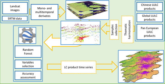
3.3. GEE Mapping Procedure

In order to develop a consistent, automated workflow to map distinct LC features as the basis for further ES analysis, our workflow was developed using full temporal Landsat images, Shuttle Radar Topography Mission (SRTM) data, multiple open-source LC products, and the GEE platform. Our workflow is divided into three parts: (1) preprocessing of satellite images, (2) reference samples selection, (3) mapping of grey, green and blue infrastructures (Figure 2).

3.3.1. Preprocessing of Satellite Images

As GEE provides free access to all Landsat surface reflectance images, we used the Landsat 5 TM surface reflectance Tier 2 product from GEE for 2000 and 2010 LC mapping. For 2020 we opted for the Landsat 8 OLI/TIRS surface reflectance Tier 2 product. All the cloud and cloud shadow pixels were removed using C implementation of the Function of Mask (CF Mask) algorithm [26].
To test which variable was important for mapping urban LC categories, we prepared a total of 32 variables. The specific variables are as follows:
  • Seven spectral reflectance (SR) bands, including blue, green, red, near infrared (NIR), short-wave infrared (SWIR1, SWIR2), and bright temperature
  • Three texture variables from the Grey-Level Co-occurrence Matrix (GLCM) measurement
  • Annual median composited surface reflectance images: we calculated fifteen spectral indices, including the Normalised Difference Vegetation Index (NDVI), Enhanced Vegetation Index (EVI), Land Surface Water Index (LSWI), Modified Normalised Difference Water Index (mNDWI), Normalised Difference Built Index (NDBI), Caly Minerals Ratio (CMR), Normalised Difference Snow Index (NDSI), Modified Soil Adjusted Vegetation Index (MSAVI), Spectral Variability Vegetation Index (SVVI), Transformed Difference Vegetation Index (TDVI), Normalised Built-up Index (NBAI), Chlorophyll vegetation Index (CIgreen), and Tasseled Cap Transformation (TCP) based Wetness, Greenness, and Brightness
  • Four seasonal indices derived from multi-temporal spectral indices
  • Four topographic variables as auxiliary parameters for the classification
All the variables used are presented in Table 2, which documents the type of variable and its formula and reference, where applicable.

3.3.2. Reference Samples Selection

As a novelty in the reference samples selection, we elaborated a sophisticated workflow for an automatic samples collection based on multi-source ground truth and raster-based LC products. As shown in Section 2.2, both ground-truth samples and remotely sensed datasets were used to generate reference samples. Firstly, the vector datasets, such as LUCAS sample points, were filtered and matched for each category. In addition, ready-made raster products such as GlobeLand30 were exploited. We collected sample points in three steps: (1) generating random points; (2) extracting values from raster products; (3) rebuilding classification code for each category. We depict the training and validation sample points in Table 3.

Assessment of Variable Importance

Ideally, more variables would lead to a better representation of the features of LC and improve the mapping accuracy. However, previous studies have shown that the accuracy and efficiency of the classification is affected by the high correlation of the data, the noise in the data collection and correction process, and the increase in computational complexity [48,49].
As a measurement for node impurity, the value of GINI can indicate how often a random instance will be misclassified. Therefore, GINI can be used to evaluate the importance of each variable [50,51]. In the RF model, GINI is calculated over all trees as the averaged reduction of node impurity on one splitting variable. Since significant variables can substantially reduce the impurity of the sample, the higher GINI values represent greater importance of the variable. This index was used as a criterion to evaluate the importance of the variables [49]. Technically, the GINI index can be calculated in GEE directly.

3.3.3. Mapping of Grey, Green and Blue Infrastructures

Random Forest Classifier

To date, Random Forest is the most widely used classifier for LC classifications [52,53,54,55]. Previous studies have shown that, compared with support vector machine (SVM), k-nearest neighbour (KNN), maximum likelihood classifier (MLC) and other models, RF has a higher classification accuracy, makes more effective use of high-dimensional data, and has higher model efficiency. Therefore, RF was used as the classifier for LC mapping based on the training samples from 3.2.2 and filtered variables. To benefit most of RF, we designed an automatic variables selection for a more efficient creation of a classification model.
Based on the knowledge from previous studies, good results can be obtained using number of trees (Ntree) as 100, and higher values do not significantly increase the accuracy of the classification [56,57,58,59,60,61]. In addition, previous studies suggested that the RF method is not very sensitive to the number of features randomly chosen to split each node (Mty) [62]. Therefore, the Ntree was set as 100 and the default parameter of Mtry was utilised in our study.

Validation

In this study, confusion matrixes were calculated based on reference validation samples to evaluate the accuracy of the classification result [63]. Several evaluation indicators were extracted, including overall accuracy (OA), producer’s accuracy (PA) and Kappa value. We used 70% of collected samples of each category as training samples, while the remaining samples (30%) were utilised for accuracy evaluation. The code to reproduce the validation in GEE is https://code.earthengine.google.com/888298b27c9b084154088bee968953d2.

Post-Classification of Dense and Dispersed Built-Up Areas

The dense built-up category refers to built-up areas with dense building stock, including informal settlements and asphalt roads. The dispersed built-up category represents impervious surface areas with ventilation space, open spaces for ventilation and green areas, which are typical of scattered residential areas, high-rise building areas, the urban fringe, and the rural hinterland [64].
To differentiate between the built-up urban areas on the basis of density, the built-up kernel density was generated applying a 17 × 17 pixels moving window according to the equation below. The size of the moving window follows the rule of the CORINE LC definition. Thus, the coverage of the built-up area was further reclassified into dense and dispersed built-up areas. The equation is as follows:
ρ b = i n 2 x i j n 2 { ρ b ρ b 50 % ,   d e n s e   b u i l t u p < 50 % ,   d i s p e r s e d   b u i l t u p
where xij represents the value of pixel i j. The value is 1 when it belongs to the built-up and 0 when it is the non-built-up LULC, n is the size of the moving window, which is set to 17 (with reference to CORINE land cover). ρb signifies the dense built-up area, if ρb is at least 50% or greater in moving window. If ρb is less than 50%, then the value is assigned to dispersed built-up area. The code for this step in GEE is https://code.earthengine.google.com/18c309ec9665c9895850390fe18f37fd.

4. Results

4.1. Feature Selection and Ranking

In Figure 3, we have summarised the results of scores to determine the importance of the variables for our RF mapping model. The results show that the seasonal index was one of the most significant variables for prediction, suggesting the value of temporal information. The seasonality enabled us to distinguish between cropland and grassland as well as between the two forest types. By doing so, we proved the seasonal index by Reschke and Hüttich [45] to highlight the differences among various types of vegetation. High-ranked variables also comprised TCP-based greenness, MNDWI, Red band, CIgreen index and seasonal index VI-MNDWI. However, several variables including four kinds of topographic variables and NIR, BT, wetness, SVVI and TDVI, were lower ranked. In hilly areas, for instance in Beijing and Ningbo, the topographic variables such as slope and DEM ranked highly.
In addition, Figure 3 reflects the change that took place in the overall classification accuracy as the categorical variables increased. The results show that the initial variable input clearly improves the classification accuracy, but when the number of variables reaches a certain level, the classification accuracy can no longer improve. Instead, some classification accuracies actually decrease as the variables increase, such as for Aarhus, Beijing and Shanghai. In order to find a balance between the classification efficiency and accuracy, the study chose the peak accuracy as the node to determine the number of input variables for further classification.

4.2. Accuracy Assessment

Among all the LC products of the study sites in 2000, 2010 and 2020, the results produced high accuracies (OA ranges from 73% to 95%). By calculating the average producer’s accuracy (PA) it was found that the highest classification accuracy was achieved for cropland, where PA could reach 92%, followed by the extraction accuracy for water bodies, which reached 87%, while the extraction accuracy for grassland and bare land were the worst with 64% and 73%, respectively (Table 4). Those two also showed the lowest classification accuracy. It is meaningful to note that the accuracy evaluation was conducted with the country as the scale. A detailed classification accuracy evaluation table and confusion matrix are available in the Appendix A.2, Table A1, Table A2, Table A3, Table A4, Table A5, Table A6 and Table A7.

4.3. Quantitative Analysis of LC and Its Changes

In order to understand the dynamics of LC change in each city over the past two decades, the area of each type of LC was summarised and illustrated in Table 5 and Table A2, Table A3, Table A4, Table A5, Table A6 and Table A7, and Figure 4a,b. Figure 5a–f shows the area of various LC types in different stages. These differences in China and Europe can be described as follows:
(1)
Built-up area ratio
By calculating the percentage of dense and dispersed built-up areas to total built-up areas, we can assess the degree of built versus more natural LC in the six cities. Based on the results for 2020, this is how the three European cities ranked in terms of share: Paris Region (75.6%), Velika Gorica (69.2%) and Aarhus (66.9%). The three Chinese cities with the highest share of built-up areas were Shanghai (73.2%), followed by Ningbo (69.08%), and finally Beijing (65.2%).
(2)
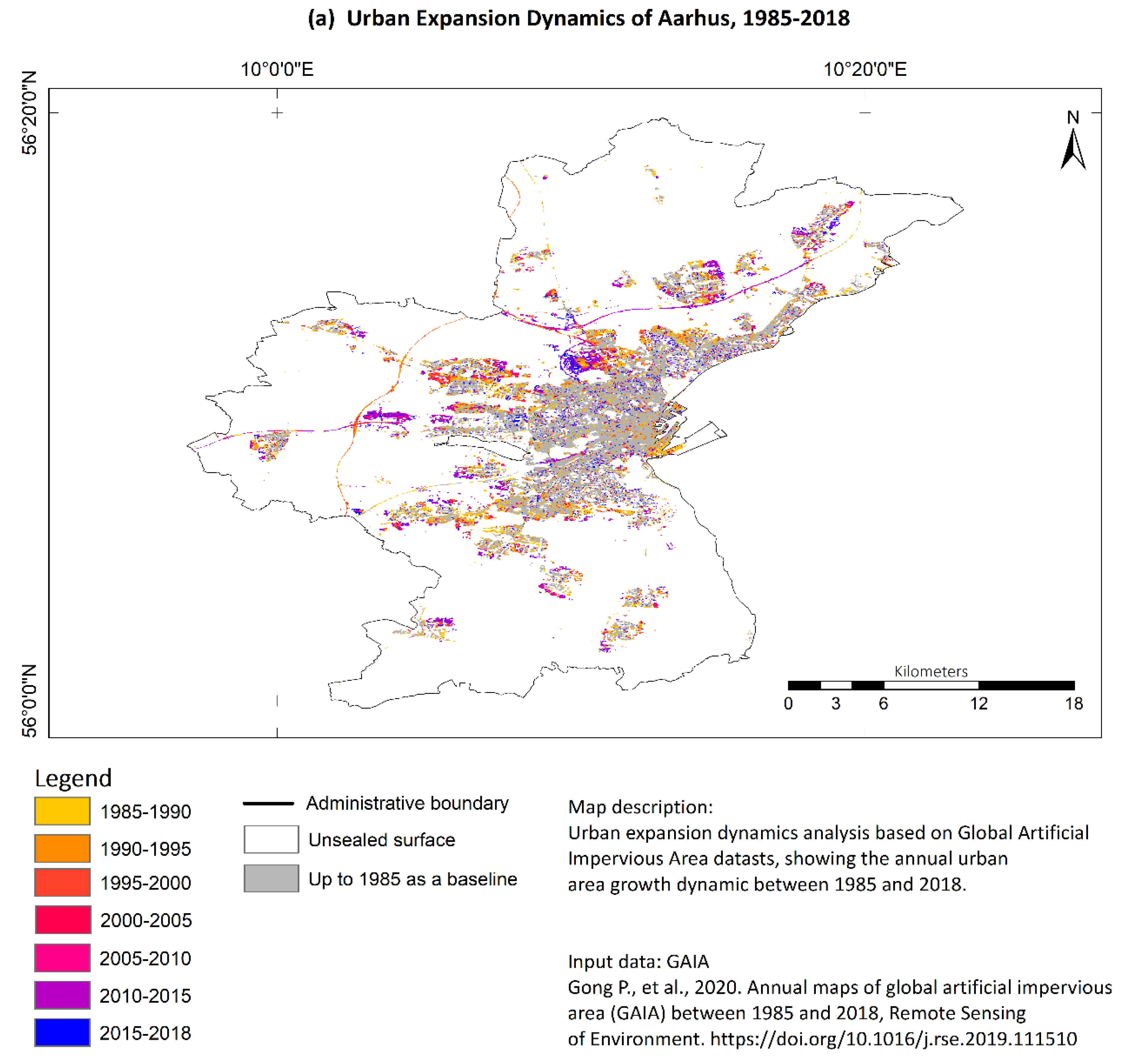
Spatial urbanisation processes
We compared the space covered by urbanisation processes in European and Chinese cities in 2020, then estimated the rate, i.e., the ratio of built-up area to total city area, and came up with the following ranking: Shanghai (40.6%), Ningbo (20.8%), Aarhus (18.1%), Beijing (17.4%), Paris Region (15.6%), and Velika Gorica (5.2%). In addition, Chinese cities have experienced dramatic urban expansion over the past 20 years. Specifically, the built-up area of the three cities has grown from 4077.6 km2 to 7508.7 km2. In the two decades between 2000 and 2020, the built-up space increased by 84%. In contrast, the built-up area of the three European cities has been rather stable over the last two decades, with the total area slightly increasing from 1780.5 km2 in 2000 to 1986.3 km2 in 2020, an increase of only 11.6%.
(3)
Reduction of green and blue spaces in connection with urban expansion
In order to understand the characteristics of LC transformation in each city from 2000 to 2020, the study further designed an LC area transfer matrix as shown in Table 5. It shows that the rapid urbanisation process had a direct impact on the cities’ green and blue LC. As a direct result of the urban expansion of the Paris Region, 646.1 km2 of cropland, 50.5 km2 of deciduous forest and 10.9 km2 of grassland have been replaced by built-up areas. A similar situation occurred in the three Chinese cities, where the urbanisation process in Beijing and Shanghai resulted in the loss of 1950.2 km2 and 1920.3 km2 of cropland each. As coastal cities, Shanghai and Ningbo have respectively converted 25.8 km2 and 100.5 km2 of water bodies into built-up surfaces due to human land reclamation.
(4)
Changes in agriculture
In the last two decades, cropland slightly increased in the three European cities from 7486.6 km2 to 7576.0 km2, an increase of merely 1.2%, while the total cropland in the three Chinese cities shrank significantly from 15,097.2 km2 in 2000 to 11,466.0 km2 in 2020, a decrease of 24%. This result indicates that the intense urbanisation process in China has led to a great loss of agriculture.
(5)
The ecological restoration effect in the selected European and Chinese cities
Although the dramatic urban expansion of the past two decades has caused damage to most ecosystem features, at the same time some areas showed the effects of significant ecological restoration driven by ecological restoration policies, or what we know as the turning green effect [65]. Specifically, in the last 20 years, 451.2 km2 of built-up areas have been restored to green and blue LC in the three European cities and 963.0 km2 were restored in the three Chinese cities.

5. Discussion

5.1. Information on Urban LC in Global Thematic Products

This study aimed to analyse LC changes to understand urban growth patterns at an intercontinental scale, as well as to provide a basis for urban ES analyses. In this analysis, we successfully tracked urbanisation processes in a historical context by interpreting global datasets such as GAIA [9] and GlobeLand30 [8,20]. Each global dataset underlies different specifications and shows the variety in their individual categorical qualities. Each dataset follows specific goals such as mapping the artificial impervious land surface cover at a global scale, or to quantify the ten most important LC categories globally. What they have in common is that they provide insights into their specific LC categories over a long period of time and spatial precision due to their 30-m resolution.
These thematic mapping products are valuable for global analyses and help us to understand how and where LC changes take place, which LC patterns exist, and in which direction loss and gain of these categories have taken place [10]. They also reveal the speed, direction and extent at which this transformation occurs [66]. These LC maps were used for visualisation purposes to gain an initial understanding of the problems that ecosystems face as a consequence of urbanisation processes, and to capture how urban growth occurs in different places.
Harmonising all the information is a challenge, as the products cover different periods and feature different levels of categorical and spatial detail. Urbanisation has a great impact on ES that relate to LC, especially to differentiated vegetation cover [67]. At the European level, highly demanding thematic mapping products have been developed that not only provide long-term information on LC, but also serve as information platforms for land use categories and their respective changes [16]. Although they are high quality and cover a long period of time, their disadvantage is that they are restricted to the European continent [18].
Regarding the Chinese cities, several thematic mapping products provide precise information for analysing LC and correspondent ES changes at fine scale with annual time steps [22]. We showed some lacks that hinder comparability of LC quantifications in Chinese and European cities. This is because of the differences in their categorical definitions and usages. In order to do justice to our targeted research, that is to use the mapping product for further ES analysis, none of the existing products were sufficient in terms of spatial extent or thematic resolution.
Hence, we overcame this challenge and managed to profit from both the global information and the details from specific European and Chinese information layers which we exploited for our distinct classification system. Another major advantage of the thematic mapping products was that we extracted all the information, layers, and categories in order to collect detailed sample points which we then used to build the map model and validate the mapping results. We take into account the inherent inaccuracies of the reference products and are aware of the potential error propagation.

5.2. Integrated Mapping Model for Relevant Urban LC Categories Tailored towards ES Feature Allocation

By using existing LC products to integrate and extract classification sample points, we could solve the problem of their difficult acquisition that was depicted in previous studies [68]). As a novelty, we propose an algorithm for automatic sample points’ acquisition. This method of classification feature screening can now be applied to other studies. By evaluating and screening multiple feature variables with the help of GINI coefficients on model evaluation, we obtained a balance of good classification accuracy as well as a high classification efficiency. We achieved this discerning classification scheme at the intercontinental level. However, we understand the restriction of our approach. As dominant artificial and natural features and thus LC may vary over different countries and cultures, they might not be represented optimally by our categories.
Our methodology ideally exploits all the spatial LC information, and therefore we were able to design a well-developed mapping procedure. With our elaborated GEE workflow, no additional infrastructure is needed. Our processing is easily reproducible in other cities contrasting other approaches [69]. The performance revealed that our design is scalable while it simultaneously only uses a viable computational time. There are no existing products for both China and Europe in the past decades showing this level of detail which we now present, especially regarding the differentiations in vegetation cover (grassland and cropland, and different types of forests). Our study conceptualised a set of automated land classification processes based on the GEE platform and geospatial big data. It is important to discuss the challenges involved in mapping LC categories at urban scale in great detail. The value of precise knowledge about ecosystems in the urbanised environment is important for gaining a deeper understanding of environmental pressures at the urban scale in a global context. Our results contribute to a better capture of LC and our approach maximises the integrated efficiency of the relevant calculations. Furthermore, the extraction of different densities in the urbanisation processes can now be tackled at intercontinental scale. In the course of urbanisation, it is of little surprise that our results show a substantial growth in artificial surfaces that subsequently caused reductions in cultivated land. We are able to quantify the loss of vegetation at the scale of the urban area. That makes it possible to monitor the direction of changes and variations of this decline at a higher level of differentiation. Another important contribution is the successful spectral separability of forest areas. Deciduous forests store more carbon than coniferous forests, so the spectral separability of forest is essential [70].

6. Conclusions

It is worth investigating the definitions and criteria of existing thematic mapping systems in order to take full advantage of their capabilities when pulling information together and extracting the appropriate data for one’s own research.
Our approach demonstrates that a requisite number of thematic classes can be derived for the mapping of specific LC categories that relate to the allocation of ES. We conclude that for reproduction purposes, a good balance between the necessary computational resources and the number of indices in use is as essential as deploying ground truth information to guarantee high quality products. Yet, there is growing imbalance between the increasing amount of satellite images and ground observations [70]. It is a challenge to gather a plentiful of samples for training and validation across continents. We hence illustrate the potential of samples collection from existing local and continental databases. We argue to keep collating ground truthing information in the light of global satellite image programs. Paying tribute to the high heterogeneity of urban areas, the more recent Sentinel data products that have been available since 2016 provide timely and continuous satellite images for LC monitoring. For less historical change detection research, the Sentinel series support mapping and monitoring at higher resolution than the Landsat series [71,72].
In order to improve the universality and model accuracy of this research method, the following aspects can be optimised in future research: First, more land-cover products as well as citizen science datasets (such as Open Street Map, OSM) can be further considered as the source of samples collection. Second, change detection methods can be employed as ways to expand the year for samples collection. Last, the accuracy evaluation system of sample points needs to be further constructed. We can, for example, use the purity and connectivity of LC to evaluate the reliability of sample points, or combine multiple product voting systems to improve the reliability of sample points, to build a higher accuracy classification model.
This level of mapping detail in urban LC facilitates for the next stage of scientific analysis to quantify the benefits and losses of related ES features. Furthermore, the outcomes of this study may also help to assess the changes in ES at an intercontinental scale, and to support the recognition of ES’s benefits and co-benefits for a more sustainable urban growth. This will be the object of research in part 2. Hence, our next task will be to estimate the equity in ES provision for this study area by further investigating the quantified spatial patterns of the diverse urbanisation processes.

Author Contributions

Conceptualization, E.B., W.W.; methodology, W.W.; software, W.W.;validation, W.W., X.L., J.K.; investigation, W.W., X.L., J.K., E.B.; writing—original draft preparation, E.B.; writing—review and editing, W.W., X.L., J.K., E.B. All authors have read and agreed to the published version of the manuscript.

Funding

1. European Union’s Horizon 2020 research and innovation programme under grant agreement No 821016”. 2. National Key Research and Development Program of China (Grant No. 2019YFA0607201) and 3. Science and Technology Commission of Shanghai (Grant No. 19DZ1203405).

Institutional Review Board Statement

Not applicable.

Informed Consent Statement

Not applicable.

Data Availability Statement

Data available on request.

Acknowledgments

We greatly appreciate research through the EC REGREEN Nature-based Solutions project (https://www.regreen-project.eu/) which enabled our collaboration. This project has received funding from the European Union’s Horizon 2020 research and innovation programme under grant agreement No 821016”. Further acknowledgement is to the National Key Research and Development Program of China (Grant No. 2019YFA0607201) and Science and Technology Commission of Shanghai (Grant No. 19DZ1203405).

Conflicts of Interest

The authors declare no conflict of interest.

Appendix A

Appendix A.1

Figure A1. (af) Visualising the dynamic urban LC expansion of the study area by means of the thematic GAIA product.
Remotesensing 13 01744 g0a1aRemotesensing 13 01744 g0a1bRemotesensing 13 01744 g0a1cRemotesensing 13 01744 g0a1dRemotesensing 13 01744 g0a1eRemotesensing 13 01744 g0a1f

Appendix A.2

Table A1. Accuracy assessment of land cover classes in six cities (OA: overall accuracy; PA: producer’s accuracy).
2000 in China
Code UrbanCroplandDeciduous
Forest
Coniferous
Forest
Grass-
Land
Bare
Land
Water
1Urban48815000100
2Cropland5919400233407
3Deciduous006319500
4Coniferous014112011000
5Grassland78871418201
6Bare land0000010
7Water2310000137
PA0.760.940.720.850.6110.81
OA0.86
Kappa0.76
2010 in China
Code UrbanCroplandDeciduous
Forest
Coniferous
Forest
Grass-
Land
Bare
Land
Water
1Urban62523400101
2Cropland1981185396508
3Deciduous0101446600
4Coniferous02519821800
5Grassland1414510713500
6Bare land0000000
7Water5310200130
PA0.74 0.73 0.82 0.77 0.60 00.94
OA0.73
Kappa0.61
2020 in China
Code UrbanCroplandDeciduous
Forest
Coniferous
Forest
Grass-
Land
Bare
Land
Water
1Urban2343900000
2Cropland3348003302
3Deciduous03188181700
4Coniferous0614182000
5Grassland12328214500
6Bare land1000000
7Water02000040
PA0.860.920.830.900.7200.95
OA0.87
Kappa0.83
2000 in Europe
Code UrbanCroplandDeciduous
Forest
Coniferous
Forest
Grass-
Land
Bare
Land
Water
1Urban24277180501
2Cropland3431966213102
3Deciduous39211844800
4Coniferous192364100
5Grassland59640221800
6Bare land2210040
7Water32401030
PA0.71 0.96 0.92 0.65 0.60 0.44 0.75
OA0.9
Kappa0.82
2010 in Europe
Code UrbanCroplandDeciduous
Forest
Coniferous
Forest
Grass-
Land
Bare
Land
Water
1Urban16012161111411
2Cropland1315395311118614
3Deciduous00522463324
4Coniferous001960002
5Grassland0016071272
6Bare land0029218126527
7Water00362245698
PA0.92 0.99 0.76 0.86 0.65 0.76 0.90
OA0.86
Kappa0.97
2020 in Europe
Code UrbanCroplandDeciduous
Forest
Coniferous
Forest
Grass-
Land
Bare
Land
Water
1Urban4598302000
2Cropland3554436252100
3Deciduous07327156800
4Coniferous32531231001
5Grassland14125217101
6Bare land0000000
7Water01023044
PA0.84 0.98 0.97 0.79 0.71 0.00 0.88
OA0.95
Kappa0.91
Table A2. Land cover area transfer matrix for the Paris Region from 2000 to 2020 (km2).
2000 2020Dense
Built-Up
Dispersed Built-UpCroplandDeciduous ForestConiferous ForestGrass-
Land
Bare
Land
Water
Dense
built-up
1699.4238.64115.066.0610.412.800.003.66
Dispersed built-up113.21294.92229.4019.0613.192.000.002.05
Cropland314.96331.179571.19327.9239.2513.120.0017.35
Deciduous forest25.6924.79479.723719.36187.299.080.006.51
Coniferous forest0.150.302.6319.0880.390.730.000.10
Grassland5.605.26345.1153.283.863.300.002.14
Bare land1.782.014.520.190.090.210.000.43
Water
bodies
1.030.581.720.311.659.320.00112.62
Table A3. Land cover area transfer matrix for Velika Gorica from 2000 to 2020 (km2).
2000 2020Dense
Built-Up
Dispersed Built-UpCroplandDeciduous ForestConiferous ForestGrass-LandBare
Land
Water
Dense
built-up
5.711.441.820.060.000.000.000.00
Dispersed built-up0.419.7212.890.280.100.050.000.22
Cropland0.995.13147.3729.060.991.550.000.09
Deciduous forest0.080.196.22180.391.491.410.000.03
Coniferous forest0.000.000.070.730.400.000.000.02
Grassland0.130.4830.0821.710.082.900.000.02
Bare land0.000.000.000.000.000.000.000.00
Water
bodies
0.000.070.180.050.530.000.002.41
Table A4. Land cover area transfer matrix for Aarhus from 2000 to 2020 (km2).
2000 2020Dense
Built-Up
Dispersed Built-UpCroplandDeciduous ForestConiferous forestGrass-
Land
Bare
Land
Water
Dense
built-up
75.075.6413.590.191.290.000.000.12
Dispersed built-up6.1819.5315.750.320.780.000.000.06
Cropland17.3126.22532.2019.9716.940.710.002.80
Deciduous forest0.400.8235.2326.799.060.190.000.69
Coniferous forest0.000.011.431.113.240.000.000.12
Grassland0.080.193.450.210.250.020.000.01
Bare land0.000.000.000.000.000.000.000.00
Water
bodies
0.090.120.040.000.180.000.000.25
Table A5. Land cover area transfer matrix for Beijing from 2000 to 2020 (km2).
2000 2020Dense
Built-Up
Dispersed Built-UpCroplandDeciduous ForestConiferous ForestGrass-
Land
Bare
Land
Water
Dense
built-up
1171.9237.72208.380.280.382.220.0011.71
Dispersed built-up343.15172.85172.041.420.389.420.0011.34
Cropland1170.53779.665617.81329.9472.88343.970.00100.77
Deciduous forest0.040.903.451926.02620.0888.640.000.02
Coniferous forest0.262.655.61994.49591.53106.580.005.23
Grassland5.7841.58349.353798.65200.381957.700.004.49
Bare land0.000.000.000.000.000.000.000.00
Water
bodies
3.973.8515.542.080.384.430.00206.39
Table A6. Land cover area transfer matrix for Shanghai from 2000 to 2020 (km2).
2000 2020Dense
Built-Up
Dispersed Built-UpCroplandDeciduous ForestConiferous ForestGrass-
Land
Bare
Land
Water
Dense
built-up
930.5214.99129.630.090.660.220.004.20
Dispersed built-up253.45129.26190.340.010.150.040.004.01
Cropland1198.69721.624096.340.378.090.560.00116.01
Deciduous forest0.000.000.000.000.000.000.000.00
Coniferous forest0.000.000.000.000.000.000.000.00
Grassland0.000.000.000.000.000.000.000.00
Bare land0.000.000.000.000.000.000.000.00
Water
bodies
14.7511.0890.260.060.260.040.00157.02
Table A7. Land cover area transfer matrix for Ningbo from 2000 to 2020 (km2).
2000 2020Dense
Built-Up
Dispersed Built-UpCroplandDeciduous ForestConiferous ForestGrass-
Land
Bare
Land
Water
Dense
built-up
544.3716.6652.200.010.640.190.007.88
Dispersed built-up201.04204.86139.360.42.923.910.008.62
Cropland672.18372.792473.8229.8352.876.380.0052.24
Deciduous forest0.000.000.000.000.000.000.000.00
Coniferous forest5.3516.84167.6232.73202.45.630.002.19
Grassland2.4911.00235.8345.3910193.500.001.46
Bare land0.000.000.000.000.000.000.000.00
Water
bodies
59.2041.49111.981.4210.200.460.00185.3
All accuracy assessments are calculated using ArcGIS 10.8.

References

  1. United Nations. World Urbanization Prospects: The 2018 Revision. Key Facts. Available online: https://population.un.org/wup/Publications/Files/WUP2018-KeyFacts.pdf (accessed on 26 January 2020).
  2. Baker, J.L. Climate Change, Disaster Risk, and the Urban Poor: Cities Building Resilience for a Changing World; World Bank: Washington, DC, USA, 2012; ISBN 978-0-8213-8845-7. [Google Scholar]
  3. Jha, A.K.; Miner, T.W.; Stanton-Geddes, Z. Building Urban Resilience: Principles, Tools, and Practice; World Bank: Washington, DC, USA, 2013; ISBN 978-0821388655. [Google Scholar]
  4. Heinrichs, D.; Krellenberg, K.; Hansjürgens, B.; Martínez, F. Risk Habitat Megacity; Springer Science & Business Media: Berlin, Germany, 2012; ISBN 978-3-642-11543-1. [Google Scholar]
  5. UN SDGs. Transforming Our World: The 2030 Agenda for Sustainable Development. Resolution Adopted by the UN General Assembly. 25 September 2015. Available online: https://sustainabledevelopment.un.org/post2015/transformingourworld (accessed on 2 February 2021).
  6. Esch, T.; Heldens, W.; Hirner, A. The Global Urban Footprint. In Urban Remote Sensing, 2nd ed.; Weng, Q., Quattrochi, D.A., Gamba, P., Eds.; Taylor & Francis: Oxfordshire, UK, 2018; pp. 1–12. ISBN 9781138054608. [Google Scholar]
  7. Angel, S.; Parent, J.; Civco, D.L.; Blei, A.; Poter, D. The dimensions of global urban expansion: Estimates and projections for all countries, 2000–2050. Progr. Plan. 2011, 75, 53–107. [Google Scholar] [CrossRef]
  8. Chen, J.; Chen, J.; Liao, A.; Cao, X.; Chen, L.; Chen, X.; He, C.; Han, G.; Peng, S.; Lu, M.; et al. Global land cover mapping at 30m resolution: A POK-based operational approach. ISPRS J. Photogramm. Remote Sens. 2015, 103, 7–27. [Google Scholar] [CrossRef] [Green Version]
  9. Gong, P.; Li, X.; Wang, J.; Bai, Y.; Chen, B.; Hu, T.; Liu, X.; Xu, B.; Yang, J.; Zhang, W.; et al. Annual maps of global artificial impervious area (GAIA) between 1985 and 2018. Remote Sens. Environ. 2020, 236, 111510. [Google Scholar] [CrossRef]
  10. Liu, X.; Huang, Y.; Xu, X.; Li, X.; Li, X.; Ciais, P.; Lin, P.; Gong, K.; Ziegler, A.D.; Chen, A.; et al. High-spatiotemporal-resolution mapping of global urban change from 1985 to 2015. Nat. Sustain. 2020, 3, 564–570. [Google Scholar] [CrossRef]
  11. Wulder, M.A.; Coops, N.C. Satellites: Make Earth observations open access. Nature 2014, 513, 30–31. [Google Scholar] [CrossRef]
  12. Caetano, M.; Mata, F.; Freire, S. Accuracy assessment of the Portuguese CORINE Land Cover map. In Global Developments in Environmental Earth Observation from Space; Marçal, A., Ed.; Millpress: Rotterdam, The Netherlands, 2006; pp. 459–467. ISBN 978-90-5966-042-7. [Google Scholar]
  13. Büttner, G.; Maucha, G. The Thematic Accuracy of Corine Land Cover 2000 Assessment Using LUCAS (Land Use/Cover Area Frame Statistical Survey); EEA Technical report No 7/2006; European Environment Agency: Copenhagen, Denmark, 2016; Available online: https://land.copernicus.eu/user-corner/technical-library/technical_report_7_2006.pdf (accessed on 26 January 2020).
  14. Aune-Lundberg, L.; Strand, G.-H. The content and accuracy of the CORINE Land Cover dataset for Norway. Int. J. Appl. Earth Obs. Geoinf. 2021, 96, 1–10. [Google Scholar] [CrossRef]
  15. European Commission. Mapping Human Presence on Earth. The Global Human Settlements Layer (GHSL). 2006. Available online: https://ec.europa.eu/jrc/sites/jrcsh/files/jrc-ghsl-infographics-key_messages.pdf (accessed on 26 January 2020).
  16. European Commission. Urban Atlas 2018 Mapping Guide. v6.7. 2020. Available online: https://land.copernicus.eu/user-corner/technical-library/urban-atlas-mapping-guide (accessed on 26 January 2020).
  17. Copernicus. Urban Atlas 2012 validation report. GMES Initial Operations/Copernicus Land Monitoring Services—Validation of Products, Report Issue 1.2. 2017. Available online: https://land.copernicus.eu/user-corner/technical-library/ua-2012-validation-report (accessed on 26 January 2020).
  18. Arsanjani, J.J.; See, L.; Tayyebi, A. Assessing the suitability of GlobeLand30 for mapping land cover in Germany. Int. J. Digit. Earth. 2016, 9, 873–891. [Google Scholar] [CrossRef] [Green Version]
  19. Ballin, M.; Barcaroli, G.; Masselli, M.; Scarnó, M. Redesign Sample for Land Use/Cover Area Frame Survey (LUCAS) 2018; Publications Office of the European Union: Luxembourg, 2018; ISBN 978-92-79-93921-1. [Google Scholar]
  20. Chen, J.; Chen, J. GlobeLand30: Operational global land cover mapping and big-data analysis. Sci. China Earth Sci. 2018, 61, 1533–1534. [Google Scholar] [CrossRef]
  21. Li, C.; Wang, J.; Hu, L.; Yu, L.; Clinton, N.; Huang, H.; Yang, J.; Gong, P. A Circa 2010 Thirty Meter Resolution Forest Map for China. Remote Sens. 2014, 6, 5325–5343. [Google Scholar] [CrossRef] [Green Version]
  22. Xu, X.; Pang, Z.; Yu, X. Spatial-Temporal Pattern Analysis of Land Use/Cover Change: Methods and Application; Scientific and Technical Documentation Press: Beijing, China, 2014; ISBN 978-7-5023-8955-0. [Google Scholar]
  23. Zhang, X.; Du, S. A Linear Dirichlet Mixture Model for decomposing scenes: Application to analyzing urban functional zonings. Remote Sens. Environ. 2015, 169, 37–49. [Google Scholar] [CrossRef]
  24. Zhang, X.; Du, S.; Wang, Q. Hierarchical semantic cognition for urban functional zones with VHR satellite images and POI data. ISPRS J. Photogramm. Remote Sens. 2017, 132, 170–184. [Google Scholar] [CrossRef]
  25. Du, S.; Du, S.; Liu, B.; Zhang, X.; Zheng, Z. Large-scale urban functional zone mapping by integrating remote sensing images and open social data. GIsci Remote Sens. 2020, 57, 411–430. [Google Scholar] [CrossRef]
  26. Foga, S.; Scaramuzza, P.L.; Guo, S.; Zhu, Z.; Dilley, R.D.; Beckmann, T.; Schmidt, G.L.; Dwyer, J.L.; Hughes, J.M.; Laue, B. Cloud detection algorithm comparison and validation for operational Landsat data products. Remote Sens. Environ. 2017, 194, 379–390. [Google Scholar] [CrossRef] [Green Version]
  27. Claverie, M.; Vermote, E.F.; Franch, B.; Masek, J.G. Evaluation of the Landsat-5 TM and Landsat-7 ETM+ surface reflectance products. Remote Sens. Environ. 2015, 169, 390–403. [Google Scholar] [CrossRef]
  28. Vermote, E.; Justice, C.; Claverie, M.; Franch, B. Preliminary analysis of the performance of the Landsat 8/OLI land surface reflectance product. Remote Sens. Environ. 2016, 185, 46–56. [Google Scholar] [CrossRef]
  29. Conners, R.W.; Trivedi, M.M.; Harlow, C.A. Segmentation of a high-resolution urban scene using texture operators. Comput. Gr. Image Process. 1984, 25, 273–310. [Google Scholar] [CrossRef]
  30. Haralick, R.M.; Shanmugam, K.; Dinstein, I.H. Textural features for image classification. IEEE Trans. Syst. Man Cybern. Syst. 1973, 6, 610–621. [Google Scholar] [CrossRef] [Green Version]
  31. Tucker, C.J. 1979. Red and Photographic Infrared Linear Combinations for Monitoring Vegetation. Remote Sens. Environ. 1979, 8, 127–150. [Google Scholar] [CrossRef] [Green Version]
  32. Huete, A.; Didan, K.; Miura, T.; Rodriguez, E.P.; Gao, X.; Ferreira, L.G. Overview of the radiometric and biophysical performance of the MODIS vegetation indices. Remote Sens. Environ. 2002, 83, 195–213. [Google Scholar] [CrossRef]
  33. Xiao, X.M.; Hollinger, D.; Aber, J.; Goltz, M.; Davidson, E.A.; Zhang, Q.Y.; Moore, B. Satellite-Based Modeling of Gross Primary Production in an Evergreen Needleleaf Forest. Remote Sens. Environ. 2004, 89, 519–534. [Google Scholar] [CrossRef]
  34. Xu, H. Modification of normalised difference water index NDWI to enhance open water features in remotely sensed imagery. Int. J. Remote Sens. 2007, 27, 3025–3033. [Google Scholar] [CrossRef]
  35. Zha, Y.; Gao, J.; Ni, S. Use of normalized difference built-up index in automatically mapping urban areas from TM imagery. Int. J. Remote Sens. 2010, 24, 583–594. [Google Scholar] [CrossRef]
  36. Alasta, A.F. Using Remote Sensing data to identify iron deposits in central western Libya. In Proceedings of the International Conference on Emerging Trends in Computer and Image Processing ICETCIP’2011, Bangkok, Thailand, 23–24 December 2011; pp. 56–61. [Google Scholar]
  37. Hall, D.K.; Riggs, G.A. Normalized-Difference Snow Index (NDSI). In Encyclopedia of Snow, Ice, and Glaciers; Singh, V.P., Singh, P., Haritashya, U.K., Eds.; Encyclopedia of Earth Sciences; Springer: Dordrecht, The Netherlands, 2011; ISBN 978-90-481-2642-2. [Google Scholar] [CrossRef] [Green Version]
  38. Qi, J.; Chehbouni, A.; Huete, A.R.; Kerr, Y.H.; Sorooshian, S. A Modified Soil Adjusted Vegetation Index. Remote Sens. Environ. 1994, 48, 119–126. [Google Scholar] [CrossRef]
  39. Coulter, L.L.; Stow, D.A.; Tsai, Y.-H.; Ibanez, N.; Shih, H.C.; Kerr, A.; Benza, M.; Weeks, J.R.; Mensah, F. Classification and assessment of land cover and land use change in southern Ghana using dense stacks of Landsat 7 ETM+ imagery. Remote Sens. Environ. 2016, 184, 396–409. [Google Scholar] [CrossRef]
  40. Bannari, A.; Asalhi, H.; Teillet, P.M. Transformed difference vegetation index (TDVI) for vegetation cover mapping. In Proceedings of the IEEE International Geoscience and Remote Sensing Symposium in Toronto, Toronto, ON, Canada, 24–28 June 2002; pp. 3053–3055. [Google Scholar]
  41. Waqar, M.M.; Mirza, J.F.; Mumtaz, R.; Hussain, E. Development of new indices for extraction of built-up area & bare soil from Landsat data. Sci. Rep. 2012, 1, 1. [Google Scholar] [CrossRef]
  42. Gitelson, A.A.; Gritz, Y.; Merzlyak, M.N. Relationships between leaf chlorophyll content and spectral reflectance and algorithms for non-destructive chlorophyll assessment in higher plant leaves. J. Plant Physiol. 2003, 160, 271–282. [Google Scholar] [CrossRef]
  43. Karlson, M.; Ostwald, M.; Reese, H.; Sanou, J.; Tankoano, B.; Mattsson, E. Mapping Tree Canopy Cover and Aboveground Biomass in Sudano-Sahelian Woodlands Using Landsat 8 and Random Forest. Remote Sens. 2015, 7, 10017–10041. [Google Scholar] [CrossRef] [Green Version]
  44. Price, K.P.; Guo, X.; Stiles, J.M. Optimal Landsat TM band combinations and vegetation indices for discrimination of six grassland types in eastern Kansas. Int. J. Remote Sens. 2010, 23, 5031–5042. [Google Scholar] [CrossRef]
  45. Reschke, J.; Hüttich, C. Continuous field mapping of Mediterranean wetlands using sub-pixel spectral signatures and multi-temporal Landsat data. Int. J. Appl. Earth Obs. Geoinf. 2014, 28, 220–229. [Google Scholar] [CrossRef]
  46. Jarvis, A.; Rubiano, J.; Nelson, A.; Farrow, A.; Mulligan, M. Practical Use of SRTM Data in the Tropics: Comparisons with Digital Elevation Models Generated from Cartographic Data; International Centre for Tropical, Agriculture (CIAT): Cali, Columbia, 2004; p. 32. [Google Scholar]
  47. Sesnie, S.E.; Gessler, P.E.; Finegan, B.; Thessler, S. Integrating Landsat TM and SRTM-DEM derived variables with decision trees for habitat classification and change detection in complex neotropical environments. Remote Sens. Environ. 2008, 112, 2145–2159. [Google Scholar] [CrossRef]
  48. Simonetti, E.; Simonetti, D.; Preatoni, D. Phenology-Based Land Cover Classification Using Landsat 8 Time Series; Publications Office of the European Union: Luxembourg, 2014; ISBN 978-92-79-40844-1. [Google Scholar]
  49. Zhang, F.; Yang, X. Improving land cover classification in an urbanized coastal area by random forests: The role of variable selection. Remote Sens. Environ. 2020, 251, 112105. [Google Scholar] [CrossRef]
  50. Menze, B.H.; Kelm, B.M.; Masuch, R.; Himmelreich, U.; Bachert, P.; Petrich, W.; Hamprecht, F.A. A comparison of random forest and its Gini importance with standard chemometric methods for the feature selection and classification of spectral data. BMC Bioinform. 2009, 10, 213. [Google Scholar] [CrossRef] [PubMed] [Green Version]
  51. Strobl, C.; Boulesteix, A.-L.; Zeileis, A.; Hothorn, T. Bias in random forest variable importance measures: Illustrations, sources and a solution. BMC Bioinform. 2007, 8, 25:1–25:21. [Google Scholar] [CrossRef] [PubMed] [Green Version]
  52. Breiman, L. Random forests. Mach. Learn. 2001, 45, 5–32. [Google Scholar] [CrossRef] [Green Version]
  53. Gumma, M.K.; Thenkabail, P.S.; Teluguntla, P.G.; Oliphant, A.; Xiong, J.; Giri, C.; Pyla, V.; Dixit, S.; Whitbread, A.M. Agricultural cropland extent and areas of South Asia derived using Landsat satellite 30-m time-series big-data using random forest machine learning algorithms on the Google Earth Engine cloud. GISci. Remote Sens. 2020, 57, 302–322. [Google Scholar] [CrossRef] [Green Version]
  54. Millard, K.; Richardson, M. On the Importance of Training Data Sample Selection in Random Forest Image Classification: A Case Study in Peatland Ecosystem Mapping. Remote Sens. 2015, 7, 8489–8515. [Google Scholar] [CrossRef] [Green Version]
  55. Tamiminia, H.; Salehi, B.; Mahdianpari, M.; Quackenbush, L.; Adeli, S.; Brisco, B. Google Earth Engine for geo-big data applications: A meta-analysis and systematic review. ISPRS J. Photogramm. Remote Sens. 2020, 164, 152–170. [Google Scholar] [CrossRef]
  56. Belgiu, M.; Dragut, L. Random forest in remote sensing: A review of applications and future directions. ISPRS J. Photogramm. Remote Sens. 2016, 114, 24–31. [Google Scholar] [CrossRef]
  57. Ismail, R.; Mutanga, O.; Kumar, L. Modeling the potential distribution of pine forests susceptible to sirex noctilio infestations in Mpumalanga, South Africa. Trans. GIS 2010, 14, 709–726. [Google Scholar] [CrossRef]
  58. Liaw, A.; Wiener, M. Classification and regression by random forest. R. News 2002, 2, 18–22. [Google Scholar]
  59. Cánovas-García, F.; Alonso-Sarría, F.; Gomariz-Castillo, F. Modification of the random forest algorithm to avoid statistical dependence problems when classifying remote sensing imagery. Comput. Geosci. 2017, 103, 1–11. [Google Scholar] [CrossRef] [Green Version]
  60. Ghimire, B.; Rogan, J.; Galiano, V.R. An evaluation of bagging, boosting, and random forests for land-cover classification in Cape Cod, Massachusetts, USA. GISci. Remote Sens. 2012, 49, 623–643. [Google Scholar] [CrossRef]
  61. Phan, T.N.; Kuch, V.; Lehnert, L.W. Land Cover Classification using Google Earth Engine and Random Forest Classifier—The Role of Image Composition. Remote Sens. 2020, 12, 2411. [Google Scholar] [CrossRef]
  62. Gislason, P.O.; Benediktsson, J.A.; Sveinsson, J.R. Random forests for land cover classification. Pattern Recognit. Lett. 2006, 27, 294–300. [Google Scholar] [CrossRef]
  63. Congalton, R.G. A review of assessing the accuracy of classifications of remotely sensed data. Remote Sens. Environ. 1991, 37, 35–46. [Google Scholar] [CrossRef]
  64. Mugiraneza, T.; Ban, Y.; Haas, J. Urban land cover dynamics and their impact on ecosystem services in Kigali, Rwanda using multi-temporal Landsat data. Remote Sens. Appl. Soc. Environ. 2019, 13, 234–246. [Google Scholar] [CrossRef]
  65. The State Council of the People′s Republic of China, 2017. Create a New Situation for Ecological Civilization Construction. Available online: http://www.gov.cn/xinwen/2017-08/02/content_5215591.html (accessed on 2 February 2021).
  66. Kadhim, N.; Mourshed, M.; Bray, M. Advances in remote sensing applications for urban sustainability. Euro-Mediterr. J. Environ. Integr. 2016, 1. [Google Scholar] [CrossRef] [Green Version]
  67. Ishola, K.A.; Okogbue, E.C.; Adeyeri, O.E. Dynamics of surface urban biophysical compositions and its impact on land surface thermal field. Model. Earth Syst. Environ. 2016, 2, 1–20. [Google Scholar] [CrossRef] [Green Version]
  68. Demuzere, M.; Bechtel, B.; Middel, A.; Mills, G. Mapping Europe into local climate zones. PLoS ONE 2019, 14. [Google Scholar] [CrossRef] [Green Version]
  69. Zhang, H.K.; Roy, D.P. Using the 500m MODIS land cover product to derive a consistent continental scale 30m Landsat land cover classification. Remote Sens. Environ. 2017, 197, 15–34. [Google Scholar] [CrossRef]
  70. Burke, M.; Driscoll, A.; Lobell, D.B.; Ermon, S. Using satellite imagery to understand and promote sustainable development. Science 2021, 371, 6335. [Google Scholar] [CrossRef]
  71. Chastain, R.; Housman, I.; Goldstein, J.; Finco, M. Empirical cross sensor comparison of Sentinel-2A and 2B MSI, Landsat-8 OLI, and Landsat-7 ETM+ top of atmosphere spectral characteristics over the conterminous United States. Remote Sens. Environ. 2019, 221, 274–285. [Google Scholar] [CrossRef]
  72. Nguyen, T.H.; Jones, S.; Soto-Berelov, M.; Haywood, A.; Hislop, S. Landsat time-series for estimating forest aboveground biomass and Its dynamics across space and time: A review. Remote Sens. 2020, 12, 98. [Google Scholar] [CrossRef] [Green Version]
Figure 1. Location of the study areas.
Remotesensing 13 01744 g001
Figure 2. Workflow for mapping of grey, green and blue infrastructures.
Remotesensing 13 01744 g002
Figure 3. The bar chart represents normalised importance scores for the 32 input variables based on GINI. The red line represents the OA of the classification in relation to the reduction of the number of input variables.
Remotesensing 13 01744 g003
Figure 4. (a) Land cover map of the three European cities in 2000, 2010 and 2020 generated by the best-fit model and well-selected variables. (b) Land cover map of the three Chinese cities in 2000, 2010 and 2020 generated by the best-fit model and well-selected variables.
Remotesensing 13 01744 g004aRemotesensing 13 01744 g004b
Figure 5. The area statistics of various land cover types in 2000, 2010 and 2020.
Remotesensing 13 01744 g005
Table 1. Distinction of mapping categories between our own source for the sophisticated LC mapping model and selected global and European data sources.
Mapping Categories Own SourceReviewed Source of Categorical Definitions
Class name (30 m res.)Random forest (RF) classifier for distinct LC mapping in GEEUrban Atlas (2006/2012/2018)
30 m to 10 m res.
GAIA (1985–2018; annual)
GLC 30 m res.
GlobeLand30
(2000/2010)
GLC 30 m res.
CORINE Land Cover
(1990/2000/2006/2012/2018) 30 m res.
Water bodiesAreas with standing and flowing watersWater bodiesWater. No definitionn.a.Areas with standing and flowing waters
Dense urban fabric≥50% of the area covered by built-up and other sealed
surfaces 17 × 17
moving window
Continuous
urban fabric (>80%)
Discontinuous dense urban
fabric (50–80%)
Global artificial
impervious areas—man-made structures.
Urban > 50%; proxy
for built-up areas.
No subdivision
Artificial surfaces: urban areas, roads, asphalt.
Specific textual
patterns >50%
Artificial
surface with land use
classification
Dispersed urban fabric<50% of the area covered by built-up and other sealed
surfaces 17 × 17
moving window
Discontinuous medium density urban fabric
(30–50%)
Discontinuous low density
urban fabric
(10–30%)
Open spaces/
barren lands
(bare soils)
Bare land (i.e., areas with uncovered soils)Land without current useBare land Bare landBare land
Perennial grassland and shrubland/cultivated land and cropland Cropland
Deciduous forest
Coniferous forest
Grassland
Arable land
Pastures
Mixed cultivation
Deciduous forest
Coniferous forest
Green urban
areas
Vegetation.
No definition
No further
distinctions
Wetlands: bogs, fens, meadows,
peat land,
floodplains
Cultivated land
Grassland
Vegetated
areas with
land use
Deciduous
forest
Coniferous
forest
Table 2. Description of spectral, texture and seasonal variables and relevant references.
CodeTypeVariablesFormulaReference
1–7Spectral ReflectanceBlueSurface reflectance bands of Landsat-5/7 TM data and Landsat-8 OLI/TIRS, where Blue, Green, Red, NIR, SWIR1, SWIR2, BT1, BT2 are band1(2), band2(3), band3(4), band4(5), band5(6), band7(7) and band6(10) of Landsat-5/7(8), respectively.[27,28]
Green
Red
NIR
SWIR1
SWIR2
Bright temperature (BT)
8–10Textureglcm_varMeasures how spread out the distribution of grey levels is[29,30]
glcm_contrastMeasures the local contrast of an image
glcm_savgSum Average
11–25Spectral
Indices
NDVI(NIR − R)/(NIR + R)[31]
EVI2.5 (NIR − RED)/(NIR + 6R − 7.5B + 1)[32]
LSWI(NIR − SWIR1)/(NIR + SWIR1)[33]
mNDWI(GREEN − SWIR1)/(GREEN + SWIR2)[34]
NDBI(SWIR1 − NIR)/(SWIR1 + NIR)[35]
CMRSWIR1/SWIR2[36]
NDSI ( SWIR 1 SWIR 2 ) / ( SWIR 1 + SWIR 2 ) [37]
MSAVI ( ( 2 NIR + 1 ) ( 2 NIR + 1 ) 2 8 ( NIR R ) )/2[38]
SVVISD(B,G,R,NIR,SWIR1,SWIR2)-SD(NIR,SWIR1,SWIR2)[39]
TDVI1.5((NIR-R)/((2NIR + R+0.5)2))[40]
NBAI(SWIR2 − (SWIR1/G))/(SWIR2 + (SWIR1/G))[41]
CIgreenNIR/G-1[42]
WetnessTasseled Cap Transformation (TCP)[43,44]
Greenness
Brightness
26–28Seasonal
Indices
VIseasonal-Dual-Season Vegetation Indices:
VI-NDVI, mNDWI, SVVI
(VIwet − VIdry)/(VIwet + VIdry)[45]
29–32 Topographic
Variables
Elevation
Slope
Aspect
Hillshade
SRTM (Shuttle Radar Topography Mission)
SRTM90_V4 data derived
[46,47]
Table 3. Number of used training sample points (T) and validation sample points (V) of each category for six cities in 2000, 2010 and 2020.
CityYearTypeBuilt-UpCroplandDeciduous ForestConiferous ForestGrasslandBare LandWater
Paris Region2000 T31731901051603894069
V1361367450261671730
Sum45345571501865565799
2010 T454148861646581221
V195638264202559
Sum649212688066831730
2020 T43847131642168703268
V188202070472301429
Total626673323462401004697
Velika Gorica2000 T10711102027662502860
V46476869281071226
Sum15315862896943574086
2010 T1324681080881242260
V572014633853926
Sum18966915431261773186
2020 T1066453642222060
V4527615189926
Sum1519215160312986
Aarhus2000 T118102732301452178
V51443141362933
Sum16914610464320730111
2010 T230780500320203890
V9933421413791639
Sum32911147144572954129
2020 T108107479893820180
V46460343816977
Sum15415341131275429257
Beijing2000 T2227311241492315231
V953135364992213
Sum31710441772133307444
2010 T446989306702891831
V19142413130124813
Sum63714134371004132644
2020 T2537434451524914528
V108318191652101912
Total36110616362177016440
Shanghai2000 T63321204018517348359
V27190917797421154
Sum90430295726424769513
2010 T63690692356616242
V2733883915287104
Sum9091294131509423346
2020 T31940648685625429
V13717421292411184
Sum45658069978036613
Ningbo2000T18210081301991643580
V784325685701534
Sum260144018628423450114
2010 T1945081013722740132
V83218459971757
Sum2777261419632457189
2020 T127256153786658453
V5411061622825194
Sum181366215409483647
Table 4. Average producer’s accuracy (PA) of the LC classifications per category.
TypeBuilt-UpCrop-
Land
Deciduous
Forest
Coniferous
Forest
Grass-LandBare
Land
Water
PA80%92%84%80%64%73%87%
Table 5. Area statistics of LULC in 2000, 2010 and 2020 in km2.
CityYearDense Built-UpDispersed Built-UpCrop-
Land
Deciduous ForestConiferous ForestGrass-
Land
Water
Bodies
Bare
Land
Paris
Region
20001235.9 444.5 7013.2 2941.9 68.5 275.9 84.0 6.1
20101300.0 323.0 7060.1 3048.5 95.6 133.4 103.2 6.1
20201424.3 460.4 7101.4 2739.0 222.5 26.8 95.6 0.0
Velika
Gorica
20006.3 16.5 129.4 132.7 0.9 38.7 2.3 0.0
20107.3 21.7 142.7 146.2 0.0 7.6 1.2 0.0
20205.1 11.9 138.7 162.4 2.5 4.1 1.9 0.0
Aarhus200053.5 23.8 344.0 40.9 3.3 2.3 0.4 0.0
201054.3 21.7 355.4 29.2 4.9 0.1 2.6 0.0
202055.3 29.3 335.9 27.1 17.7 0.5 2.3 0.0
Beijing20001097.2 543.7 6435.7 2007.0 1301.5 4840.2 180.1 0.0
20101664.8 650.3 6397.4 3755.7 475.2 3303.7 158.3 0.0
20202064.0 794.8 4872.4 5369.0 1131.0 1915.4 258.8 0.0
Shanghai2000921.3 492.3 5236.9 0.0 0.0 0.0 233.2 0.0
20101751.0 654.5 4083.1 71.5 1.7 34.2 287.7 0.0
20202045.1 747.9 3841.9 0.5 7.8 0.7 239.8 0.0
Ningbo2000537.8 485.3 3424.6 0.0 2974.0 1142.7 354.7 0.0
2010828.7 427.9 3795.9 32.1 2730.2 788.5 315.8 0.0
20201282.9 574.0 2751.7 94.9 3975.4 17.4 222.9 0.0
Publisher’s Note: MDPI stays neutral with regard to jurisdictional claims in published maps and institutional affiliations.

