Article

Diurnal Variation of the Diffuse Attenuation Coefficient for Downwelling Irradiance at 490 nm in Coastal East China Sea

1
State Key Laboratory of Tropical Oceanography (LTO), South China Sea Institute of Oceanology, Chinese Academy of Sciences, Guangzhou 511458, China
2
University of Chinese Academy of Sciences, Beijing 100049, China
3
Southern Marine Science and Engineering Guangdong Laboratory (Guangzhou), Guangzhou 511458, China
4
Guangdong Key Lab of Ocean Remote Sensing, Guangzhou 511458, China
5
College of Oceanography, Hohai University, Nanjing 210098, China
6
South China Sea Branch of State Oceanic Administration, Guangzhou 510301, China
*
Author to whom correspondence should be addressed.
Remote Sens. 2021, 13(9), 1676; https://doi.org/10.3390/rs13091676
Submission received: 19 March 2021 / Revised: 21 April 2021 / Accepted: 21 April 2021 / Published: 26 April 2021
(This article belongs to the Special Issue Seawater Bio-Optical Characteristics from Satellite Ocean Color Data)

Abstract

:
The diurnal variation of the diffuse attenuation coefficient for downwelling irradiance at 490 nm ( K d ( 490 ) ) has complex characteristics in the coastal regions. However, owing to the scarcity of in situ data, our knowledge on the diurnal variation is inadequate. In this study, an optical-buoy dataset was used to investigate the diurnal variation of K d ( 490 ) in the coastal East China Sea, and to evaluate the K d ( 490 ) L2 products of geostationary ocean color imager (GOCI), as well as the performance of six empirical algorithms for K d ( 490 ) estimation in the Case-2 water. The results of validation show that there was high uncertainty in GOCI L2 K d ( 490 ) , with mean absolute percentage errors (MAPEs) of 69.57% and 68.86% and root mean square errors (RMSEs) of 0.70 and 0.71 m−1 compared to buoy-measured K d 12 ( 490 ) and K d 13 ( 490 ) , respectively. Meanwhile, with the coefficient of determination (R2) of 0.71, as well as the lowest MAPE of 27.31% and RMSE of 0.29 m−1, the new dual ratio algorithm (NDRA) performed the best in estimating K d ( 490 ) in the target area, among the six algorithms. Further, four main types of K d ( 490 ) diurnal variation were found from buoy data, showing different variabilities compared to the area closer to the shore. One typical diurnal variation pattern showed that K d ( 490 ) decreased at flood tide and increased at ebb tide, which was confirmed by GOCI images through the use of NDRA. Hydrometeorological factors influencing the diurnal variations of K d ( 490 ) were also studied. In addition to verifying the predominant impact of tide, we found that the dominant effect of tide and wind on the water column is intensifying sediment resuspension, and the change of sediment transport produced by them are secondary to it.

Graphical Abstract

1. Introduction

The diffuse attenuation coefficient for downwelling irradiance ( K d ) defines the rate of decrease of downwelling irradiance with water depth, which can be used, among other things, to compute primary production and describe the clarity of seawater [1,2,3,4,5]. Following the primary studies in the 1970s [6], the value of K d at 490 nm ( K d ( 490 ) ) is traditionally measured in situ at marine platforms or provided as a comment product by remote sensing satellite instruments [7]. Generally, K d ( 490 ) is strongly correlated with the concentration of suspended particulate matter (SPM) in turbid coastal waters [8,9]; thus, the K d ( 490 ) of these waters is usually used to study the process of sediment transportation and resuspension [10]. In addition, in highly dynamic coastal waters, K d ( 490 ) shows significant diurnal variations because of tidal forcing, atmospheric and current disturbances [11,12].
At present, remote sensing provides a simple and convenient method to study the variation of K d ( 490 ) , especially via the geostationary satellites such as Geostationary Ocean Color Imager (GOCI), which can provide a synoptic view of diurnal variations on K d ( 490 ) . However, the remote-sensed algorithms for K d ( 490 ) in clear Case-1 waters always underperform in turbid Case-2 waters with complex optical properties [2,12,13]. To retrieve the real K d ( 490 ) in coastal waters, signals in the red and near-infrared bands were used in several empirical algorithms, and produced good inversion effects [13,14,15,16]. However, accuracies of these algorithms still need further validations using a large in situ dataset.
In the coast of the East China Sea, our understanding of K d ( 490 ) is limited to general spatial distribution [13], while the diurnal or hourly variabilities of K d ( 490 ) are not fully understood, especially for the transitional area between the highly turbid estuarine water and the clear off-shore area. To the best of our knowledge, only one study based on GOCI-derived and reconstructed K d ( 490 ) has revealed that K d ( 490 ) decreases as the tide elevation increases and increases as tide decreases in the coast of the East China Sea [11]. Since traditional in situ measurement of K d ( 490 ) during a single cruise was not able to resolve the diurnal variations of K d ( 490 ) . Marine optical buoys provide novel insights not only to validate satellite products, but also to understand the interplay between the diurnal variations of K d ( 490 ) and dynamic processes [17,18,19].
In this study, an optical buoy was moored in the coastal East China Sea (30°40.7′N, 122°49′E) from15 September 2013 to 11 January 2014 (139 days in total) to obtain the field diurnal variation of K d ( 490 ) . Based on the optical-buoy dataset, we first evaluated the K d ( 490 ) product from the GOCI as well as six empirical algorithms for K d ( 490 ) estimation in Case-2 water. Subsequently, we studied the characteristics of diurnal variations of K d ( 490 ) in the coastal East China Sea and tried to reveal the relationship between the environment factors and K d ( 490 ) .

2. Materials and Methods

2.1. Study Area

The site of the optical buoy is close to the Shengshan and Gouqi islands (Figure 1), owing to the Shengsi islands. Water depth is about 20 m. The Shengsi islands are located across the boundary of the Yangtze Estuary and Hangzhou Bay, both of which are known as highly turbid coastal areas due to the large amounts of suspended sediment discharged by several runoffs and resuspended from local seabed. The Yangtze River is the largest source of sediments for these two regions, it carries approximately 486 Mt of sediments annually into the East China Sea [20], forming the largest turbidity zone in the center of the Yangtze Estuary. It develops eastward into a suspended sediment plume, which can extend to 123°E and affect our target area [21]. Our target area, marked by a black rectangle in Figure 1, has a high-incidence of red tide [15,22]. It is located in the monsoon climatic zone, where the northerly/southerly wind prevails in winter/summer, respectively, and both spring and autumn are transitional periods. The average wind speed over the years is about 6.5 m/s [23]. As the leading type of suspended sediment here in this region, clay makes the water body susceptible to external influences and produces sediment resuspension processes [24] Therefore, SPM of this highly dynamic coastal area varies significantly, under the control of multiple dynamic processes, such as tide, monsoon, the Yangtze river dilute water, and other water masses [11,24,25]. Mussel aquaculture in the Shengsi islands is prosperous, and has become a pillar industry [26]. Conceivably, the bio-optical properties of the Shengsi aquatic environment are quite complicated and variable.

2.2. Structure and Measurements of the Optical Buoy

The optical buoy used in this study was designed by the Optics Laboratory at the South China Sea Institute of Oceanology, Chinese Academy of Sciences (Figure 2). There existed wind speed and direction sensors on the top the buoy, as well as communication equipment (Figure 2a). The buoy was equipped with an incident irradiance ( E s ( z , λ ) ) sensor above the water surface, three downwelling irradiance ( E d ( z , λ ) ) sensors, and three upwelling radiance ( L u ( z , λ ) ) sensors at depths of 1.65, 3.25, and 4.85 m, respectively (Figure 2b). Radiometric measurements were performed synchronously by all the radiometers at hourly intervals, from 8:00 to 17:00 Beijing Time (BJT). More than 10 sets of data were continuously collected during each measurement. The spectral range of each radiometer was 350–1100 nm, and the hyperspectral resolution was 0.375 nm. In addition, an independent measurement was carried out at 2:00 BJT for dark current correction.

2.3. Optical Buoy Data Processing

The availability of buoy data is relatively low; after a series of quality control steps, only about 50% of the raw data are valid. The screening criteria can be outlined by following four steps: (1) erroneous data caused by abnormal data transmission were deleted; (2) significantly abnormal spectra in each group of continuously measured data were manually discarded; (3) data with depth < 0 m were removed to avoid situations where the underwater radiometers were exposed to the water surface; and (4) data with an inclination angle greater than 10° were regarded as low quality and eliminated to reduce the self-shading effect. Then, the remaining effective spectra were interpolated to an integer wavelength, and the hyperspectral data were smoothed by a moving average method with a window width of 15 nm.
After quality control and the preprocessing of raw data, valid E s ( z ,   λ ) , E d ( z ,   λ ) , and L u ( z ,   λ ) spectra were used to derive K d ( λ ) and R rs ( λ ) . In this study, K d ( λ ) is the vertical average of the diffuse attenuation coefficient of the water column between two selected irradiance sensors on the optical buoy, and is calculated as
K d 12 ( λ ) = ln E d ( 1.65 , λ )     ln E d ( 3.25 , λ ) 1.6 ,
K d 13 ( λ ) = ln E d ( 1.65 , λ )     lnE d ( 4.85 , λ ) 3.2 ,
Similarly, the diffuse attenuation coefficient of upwelling radiance ( K l ( z ,   λ ) ) can be calculated using
K l 12 ( λ ) = ln L u ( 1.65 , λ )     ln L u ( 3.35 , λ ) 1.6 ,
K l 13 ( λ ) = ln L u ( 1.65 , λ )     ln L u ( 4,85 , λ ) 3.2 ,
where E d ( 1.65 ,   λ ) ( L u ( 1.65 ,   λ ) ), E d ( 3.25 ,   λ ) ( L u ( 3.25 ,   λ ) ) and E d ( 4.85 ,   λ ) ( L u ( 4.85 ,   λ ) ) are the downwelling irradiance (radiance) measured at 1.65, 3.25 and 4.85 m, respectively. Here, 1.6 and 3.2 m refer to the vertical distance between the two utilized irradiance (radiance) sensors. K d 12 ( λ ) ( K l 12 ( λ ) ) and K d 13 ( λ ) ( K l 13 ( λ ) ) are calculated between the first and second and the first and third irradiance (radiance) sensors, respectively.
R rs ( λ ) is defined by the following equation:
R rs ( λ ) = L w ( λ ) E s ( λ )
Here, E s ( λ ) is the incident irradiance measured above the surface of the water, and L w ( λ ) is the water-leaving radiance, which is derived from Equation (6).
L w ( λ ) = 1 ρ w n 2 L u ( 0 , λ ) = 0.543 L u ( 0 , λ ) ,
where ρ w is the Fresnel reflectance of the air−sea interface, and n is the refractive index of seawater. 1   ρ w n 2 represents the transmittance for the upwelling radiance of the seawater and air interface, and its value can be regarded as a constant −0.543 [27]. L u ( 0 , λ ) is the upwelling radiance just beneath the surface, which is not directly measurable, and the theoretical value is usually derived from the Beer–Lambert law using the following equation:
L u ( 0 , λ ) = L u ( z , λ ) e K l ( λ ) z ,
Here, L u ( z , λ ) is the upwelling radiance at depth z, and K l ( λ ) refers to one of K l 12 ( λ ) , K l 13 ( λ ) calculated above. Further, R rs ( λ ) derived from K l 12 ( λ ) and K l 13 ( λ ) are labeled as R rs 12 ( λ ) and R rs 13 ( λ ) , respectively.

2.4. Satellite Data Processing

Level-2 products of GOCI between 15 September, 2013 and 11 January, 2014 were downloaded from the NASA’s Ocean Color website (https://oceancolor.gsfc.nasa.gov, accessed on 26 April 2021). The NASA standard atmospheric correction algorithm was adopted by NASA during the generation of its official GOCI L2 products [28]. Downloaded GOCI L2 K d ( 490 ) is derived from the GOCI L2 R rs through the use of NASA officially K d algorithm, KD2S (https://oceancolor.gsfc.nasa.gov/atbd/kd_490/#sec_2, accessed on 26 April 2021). A 32-bit quality flag (l2_flag) is contained in each Level-2 file, which was applied to exclude questionable pixels.
The following time-space matching criteria for GOCI and buoy data were adopted in this study [29]: (1) A 3 × 3 box centered around the buoy location is selected to represent the satellite-derived estimations. (2) Pixels are discarded if any of the following flags are set in the selected window: atmospheric correction failure, land, cloud or ice, stray light, sun glint, high top-of-atmosphere radiance, low L wn (555) ( L wn refers to normalized water-leaving radiance), or solar zenith angle above the limit [29]. (3) The time window between GOCI and buoy is set to <±30 min [30,31] to minimize the effects of the temporal variability of the atmosphere and seawater around the buoy site. The GOCI estimations and buoy measurements that meet this condition were considered “concurrent.” (4) The GOCI estimations are valid only when the number of valid pixels is 5 in the selected 3 × 3 window, and these valid pixels are obtained through the spatial homogeneity test. Spatial homogeneity means that all valid pixels should be within ±1.5 *standard deviation of the median for the 3 × 3 window. Moreover, the coefficient of variation (CV; filtered standard deviation divided by the filtered mean) of valid data in a 3 × 3 window should be <0.15. Then, if the corresponding buoy measurements are also valid, the GOCI and buoy measurements match successfully.

2.5. Ancillary Data Acquisition

Several hydrometeorological parameters were used in this study, including temperature, salinity, wind direction, wind speed, accumulated rainfall, and tide elevation. The first two parameters were measured using the moored optical buoy. Wind direction, wind speed, and accumulated rainfall were measured at the Shengshan meteorological station by the National Meteorological Information Center (http://data.cma.cn, accessed on 26 April 2021). The tide elevation was observed at the Lv huashan tide gauge station by the National Marine Information Center.

2.6. Performance Assessment

Several statistical measures were used to assess the differences between the GOCI/buoy estimations and buoy measurements, including root mean square error (RMSE), mean absolute percentage error (MAPE), mean ratio (MR), slope/intercept coefficients, and the coefficient of determination ( R 2 ) between the two datasets when a linear regression was applied. The RMSE, MAPE and MR are defined as follows.
RMSE = 1 N n = 1 N ( y n     x n ) 2 ,
MAPE = 1 N n = 1 N | y n     x n | x n * 100 % ,
MR = 1 N n = 1 N y n x n ,
where yn represents the derived values, and xn represents the in situ values.
In the study of K d variations, the coefficient of variation (CV) is used, which is calculated as follows:
CV = [ 1 N i = 1 N ( X i     1 N i = 1 N X i ) 2 ] 1 / 2 1 N i = 1 N X i ,   i = 1 ,   2 ,   ,   N
When the value of the CV of a set of data is larger, its variation is more significant.

3. Results

3.1. Reliability and Uncertainty of the Optical Buoy Data

The reliability of the optical buoy data has always been an important concern in its applications, because its radiometric measurements are affected by numerous factors [32]. The two most important factors are the effect of instrument self-shadow and sea surface wave convergence [33]. To reduce uncertainties from the instrument self-shadow effect, small optical fiber probes and various other advanced technologies were adopted and achieved reliable results [34,35,36]. Moreover, two angle sensors were set to obtain the inclination angles of the buoy body. Data with tilt angle greater than 10° were deleted as mentioned in Section 2.3. Evaluation was carried out for the inevitable effects of the convergence of sea surface waves on K d ( 490 ) in our previous study, where the depth variation was used to reflect the wave disturbance [37]. The CVs of 488 groups of K d 12 ( 490 ) and depth continuously measured at adjacent moments were calculated, and the results showed that the CV of K d 12 ( 490 ) remains low, even when the depth changes significantly (Figure 3). This indicates that the uncertainty of the measurement data of buoys from the convergence of sunlight produced by sea waves is acceptable.
The coastal water of the East China Sea is stratified, where the lower water layer is more turbid than the upper layer, under the agitation of the underlying water mass. The method of underwater radiation measurement at fixed depths adopted by the optical buoy is not recommended in stratified water [32]. In this type of water column, the actual changes of E d and L u may differ significantly from those obtained from the hypothetic exponential variation. In order to assess this uncertainty, we compared the buoy-measured K d 12 ( 490 ) and K d 13 ( 490 ) to evaluate the level of stratification of the upper layer. Consequently, K d 12 ( 490 ) and K d 13 ( 490 ) showed a consistency (Figure 4), indicating a slight stratification in the depth range of buoy measurement. Moreover, the mixing degree of water bodies within the observation depth range of the buoy was relatively high. This indicated that the method of underwater radiometric measurement at fixed depths is valid in our target area.
A depth sensor was used to obtain the true depth of the buoy in operation in order to correct the depth deviations resulting from the buoy body floating up and down due to external disturbances. To reduce the biological contamination on the optical surface, the optical window of each radiometer is equipped with a mechanical automatic cleaning brush designed by us. In addition, it should be noted that treating the transmission coefficient as a constant (0.543) in Equation (6) also introduced a small amount of uncertainty [38]. Improvement measures have been adopted in the design of the buoy structure and the optical radiation measurement system, in response to possible sources of uncertainties in buoy data. For inevitable uncertain sources, screening and evaluation was performed before the use of buoy data to ensure the reliability of the data.

3.2. Overview of In Situ Buoy Measurement

We introduce the overview of K d 12 ( 490 ) in this section because K d 12 ( 490 ) is very similar to K d 13 ( 490 ) and it has greater remote sensing significance. Valid K d 12 ( 490 ) data, at 691 different time points, were obtained in total, which were averaged from each set of continuously measured spectra per hour. From our statistical results, K d 12 ( 490 ) varied from 0.177 to 4.307 m 1 , and the average value of K d 12 ( 490 ) was 1.283 ± 0.836 m 1 . We found that more than 98% of the K d 12 ( 490 ) values were greater than 0.3 m 1 , showing that the water body is not clear during our observation. More than 50% of the value of K d 12 ( 490 ) is less than 1 m 1 , and the percentage of K d 12 ( 490 ) larger than 2 m 1 is less than 20% (Figure 5). This demonstrated that the water in this transition sea area has not ever reached a highly turbid state. However, the large magnitude range in K d 12 ( 490 ) indicates highly dynamic in the water body.

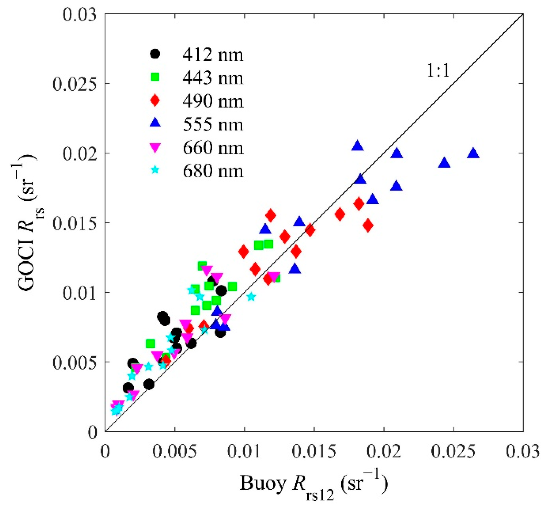
3.3. Evaluation and Correction of the Official GOCI L2 K d ( 490 )

3.3.1. Error of the GOCI L2 K d ( 490 )

There exists a significant difference between GOCI L2 K d ( 490 ) and the buoy K d 12 ( 490 ) , as well as K d 13 ( 490 ) . It can be clearly observed from the black and grey dots depicted in Figure 6 that GOCI L2 K d ( 490 ) is far lower than buoy K d 12 ( 490 ) and K d 13 ( 490 ) , with RMSEs of 0.70 and 0.71 m 1 , MAPEs of 69.57% and 68.86%, respectively.

3.3.2. Evaluation of Six Empirical K d ( 490 ) Algorithms

To improve the accuracy of the GOCI L2 K d ( 490 ) in the target area, we evaluated the accuracies of six empirical algorithms, including a new diurnal ratio algorithm (NDRA) proposed for the coastal East China Sea in our previous article [37]. None of these algorithms were built specifically for GOCI. Therefore, the calibration dataset (1151 groups of effective R rs 12 ( λ ) and K d 12 ( 490 ) ) of NDRA was used to re-calibrate the formulas on GOCI central bands of Wang X.M.’s algorithm [39], Chen’s algorithm [40], Wang M.H.’s algorithm [41], Zhang’s algorithm [16] and Tiwari’s algorithm [14], as well as NDRA, in order to eliminate the differences in the application effect of each algorithm due to the different modeling datasets (Table 1).
The NDRA validation dataset (581 groups of effective R rs 12 ( λ ) and K d 12 ( 490 ) ) was also used to calculate the inversion accuracy of each algorithm. The comparisons are shown in Figure 7a–f and results from the statistical analysis are summarized in Table 2. The inversion result of Wang X.M.’s algorithm is not ideal. When K d ( 490 ) is less than 1 m 1 , the derived K d ( 490 ) is 1–3 times of the in situ one; in the turbid water where K d ( 490 ) is greater than 1 m 1 , a significant underestimation takes place (Figure 7a). Chen’s algorithm produces overestimation in water bodies where K d ( 490 ) is less than 0.5 m 1 , while in water bodies where K d ( 490 ) is greater than 0.5 m 1 there exists an improving application effect (Figure 7b). Wang M.H.’s algorithm overestimates the entire range of K d ( 490 ) (Figure 7c). For the Zhang’s algorithm, the estimated K d ( 490 ) calculated by it is close to the in situ value when K d ( 490 ) is less than 1 m 1 . On the other hand, when K d ( 490 ) is greater than 1 m 1 , an overestimation occurs, whereby the derived K d ( 490 ) can be 2.5 times of the in situ K d ( 490 ) (Figure 7d). Both NDRA and Tiwari’s algorithm have high accuracies (Figure 7e,f)). The RMSEs of the two algorithms are 0.29 m 1 and 0.30 m 1 , respectively; the MAPEs are 27.31% and 28.15%, respectively; and the R 2 s are 0.72 and 0.71, respectively (Table 2). However, as K d ( 490 ) increases to >1 m 1 , K d ( 490 ) tends to be underestimated by Tiwari’s algorithm (Figure 7e). Among all these algorithms, NDRA has the highest accuracy and best stability in this sea area, this is consistent with the results that we obtained previously [37].

3.3.3. Improvement of GOCI L2 K d ( 490 )

NDRA has the highest accuracy in the coast of the East China Sea, as shown in Section 3.3.2. Consequently, it was adopted to improve the quality of GOCI-derived K d ( 490 ) . K d ( 490 ) retrieved from GOCI R rs by NDRA is plotted against buoy K d 12 ( 490 ) and K d 13 ( 490 ) in Figure 8. The accuracy of K d ( 490 ) derived from GOCI R rs is greatly improved by NDRA. Comparing K d ( 490 ) derived from GOCI L2 R rs by NDRA and K d 12 ( 490 ) as well as K d 13 ( 490 ) , the MAPEs are 42% and 43.30% and the RMSEs are 0.34 and 0.33 m−1, respectively. The difference between newly derived GOCI K d ( 490 ) and K d 12 ( 490 ) is close to the difference between it and K d 13 ( 490 ) . However, K d ( 490 ) retrieved from GOCI L2 R rs using NDRA is still somewhat high compared to buoy-measured K d ( 490 ) . This could be caused by other factors besides the K d ( 490 ) algorithm used.

3.4. Diurnal Variations of K d ( 490 ) Obtained by Buoy

3.4.1. Statistics of Diurnal Variations

The data of 43 days, with daily valid data of 7 h, were obtained and selected to study the diurnal variations of K d ( 490 ) in the study area. Through statistics, we found that the absolute amplitudes of daytime variability (Δ) for K d ( 490 ) during the 43 selected days ranged from 0.12 to 3.03 m 1 , accounting for approximately 25.22% to 250.49% (the mean is 100.16 ± 55.76%) of the corresponding diurnal averages. In addition, the daily CV of K d ( 490 ) ranged from 0.1 to 0.78, and the corresponding mean CV was 0.34 ± 0.19. Within a day, the maximum value of K d ( 490 ) can be seven times its minimum value, indicating a significant diurnal dynamic of K d ( 490 ) . It was also found that the variations of Δ and CV for K d ( 490 ) have similar trends with the values of K d ( 490 ) . When the value of K d ( 490 ) is greater, the diurnal variation is more apparent, with a few exceptions. Moreover, a majority (30 out of 43) of the K d ( 490 ) daytime maximum values were achieved in the afternoon (after 12:00 BJT), >70% of which occurred after 14:00 BJT. The minimum value of K d ( 490 ) was achieved evenly in the forenoon and afternoon, with 21 out of 43 in the forenoon and 22 out of 43 in the afternoon.

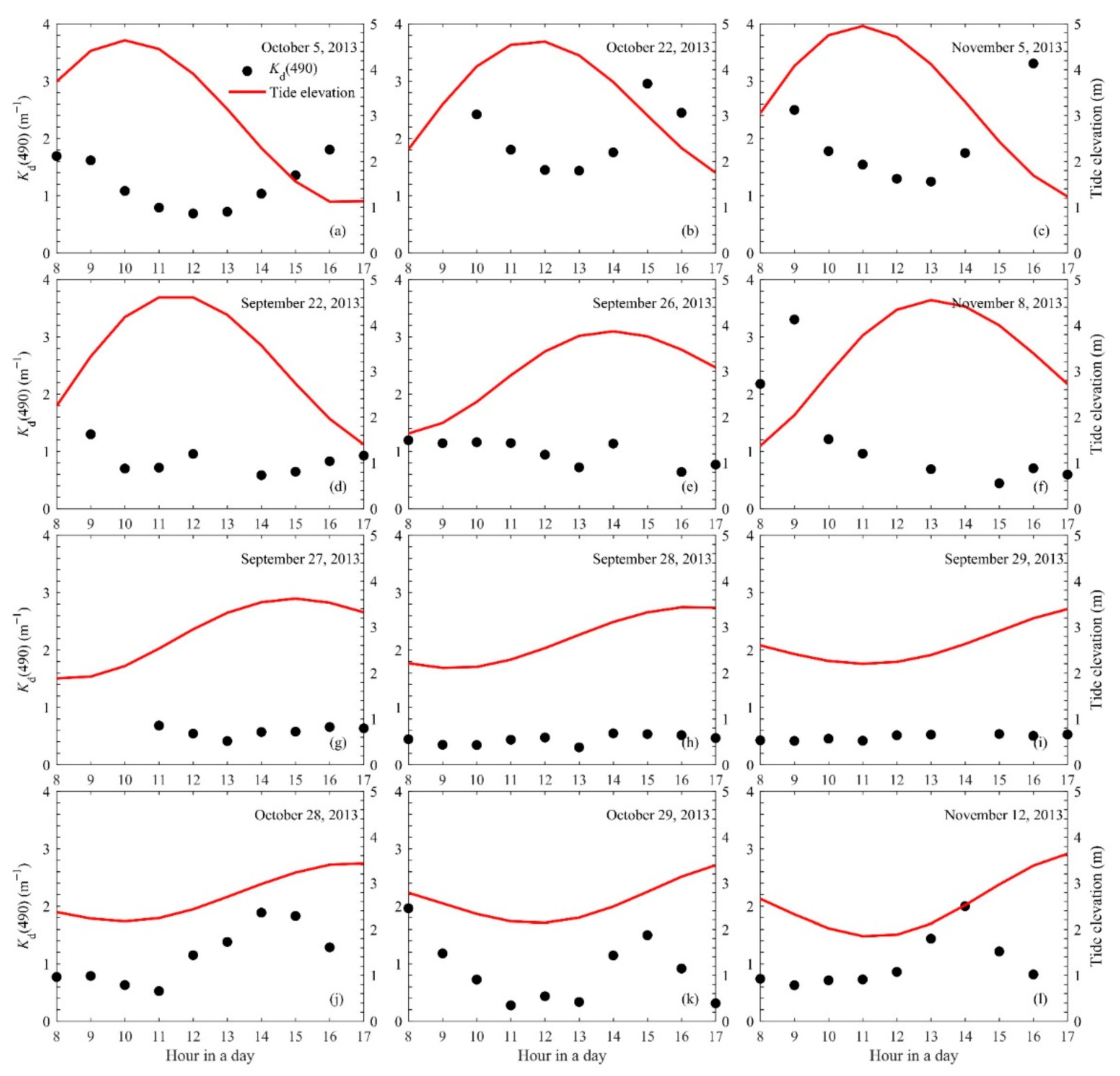
3.4.2. Four Kinds of Diurnal Variation
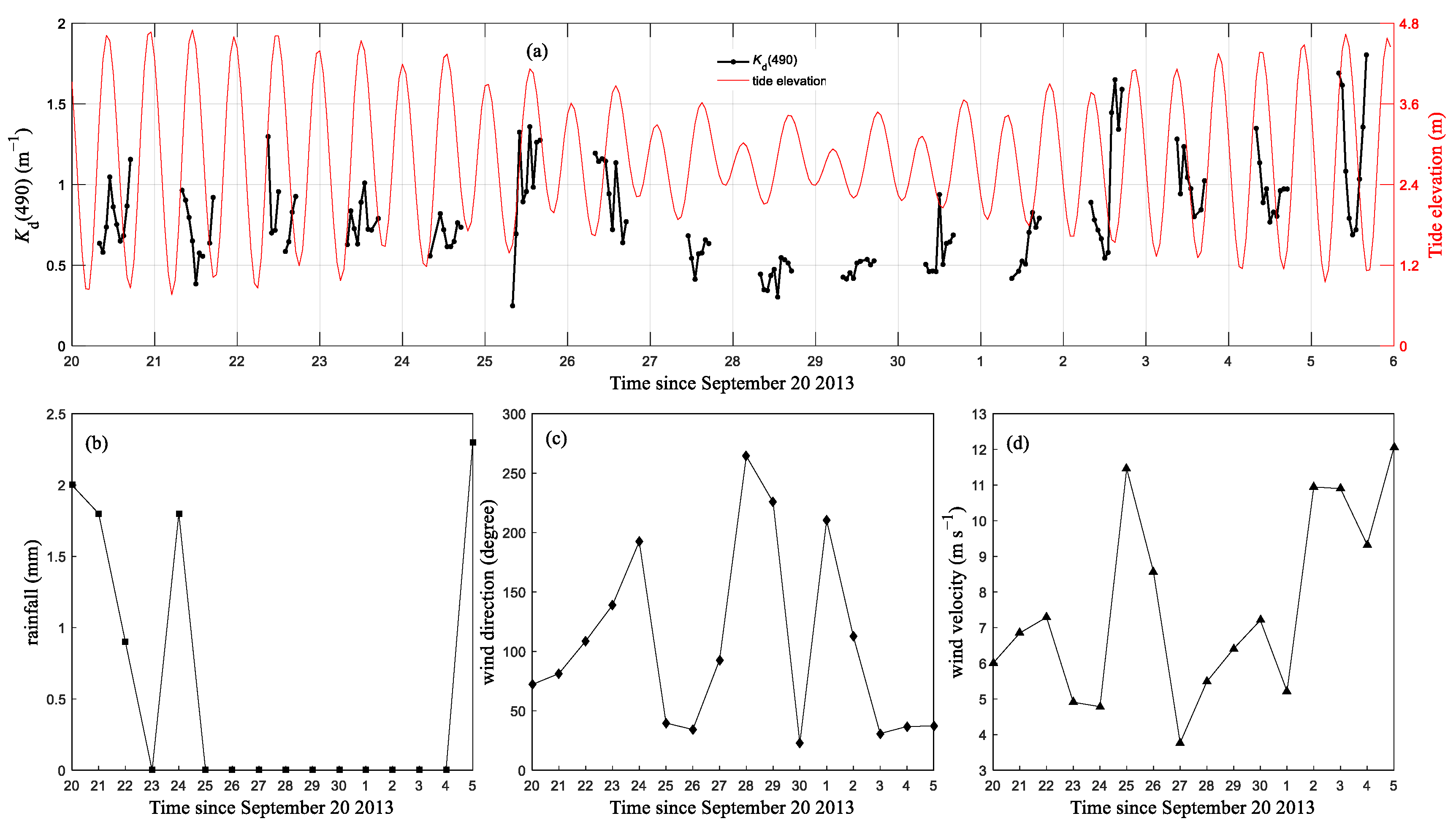
Among the 43-day dataset mentioned in Section 3.4.1, 12 days of continuous valid data were selected to illustrate the diurnal variation characteristics of K d ( 490 ) . It was observed that the diurnal variations of K d ( 490 ) in the target area can be roughly divided into four categories. The first typical variation pattern is shown in Figure 9a–c, in which K d ( 490 ) was found to gradually decrease during the flood tide and increase during the ebb tide. In addition, the minimum K d ( 490 ) appeared 1–2 h after the tide reached its maximum. The second type of diurnal variation has a similar property to the first variation pattern (Figure 9d–f), in which K d ( 490 ) varies with the tide elevation in general. However, some outliers exist in this pattern. The third variation pattern is for lower K d ( 490 ) values corresponding to clear water (Figure 9g–i), which did not exhibit remarkable variations over the entire time period. The last variation pattern is not readily comprehensible (Figure 9j–l); K d ( 490 ) increased/decreased as the tide elevation increased/decreased and then switched to the opposite pattern.

3.4.3. Diurnal Variations of K d ( 490 ) in a Spring–Neap Tide Cycle

The buoy K d ( 490 ) shows a significant spring–neap cycle. Four sets of K d ( 490 ) data corresponding to four different spring–neaps were obtained, with spring data from 20 September, 5 October, 20 October, and 5 November, 2013, and neap data from 28 September, 13 October, 28 October, and 11 November, 2013. The daily averages of K d ( 490 ) for the four spring tides are 0.797 ± 0.187, 1.198 ± 0.434, 2.145 ± 0.974, and 1.916 ± 0.741 m 1 , respectively. Additionally, for the four neap tides, the daily averages of K d ( 490 ) are 0.441 ± 0.084, 0.879 ± 0.537, 1.138 ± 0.501, and 1.076 ± 0.268 m 1 , respectively. The daily mean K d ( 490 ) of the spring of autumn was 1.36–1.88 times that of the neap, with an average of 1.69 times. For the sole spring–neap of winter, it was found that the daily average value of K d ( 490 ) of the spring was 1.78 times that of the neap. The fluctuation from spring to neap is larger during winter than during autumn.
The diurnal variation of buoy K d ( 490 ) and the corresponding meteorological parameters were plotted together (Figure 10) to further understand the detailed dynamics of K d ( 490 ) in a spring–neap tide cycle. K d ( 490 ) from 8:00 to 17:00 BJT with hourly intervals from 20 September to 5 October, 2013 is shown in Figure 10a, including a continuous tide elevation curve from 00:00 to 23:00 BJT on each day. Note that K d ( 490 ) at some moments were not illustrated, owing to poor data quality or equipment failure. Additionally, the daily accumulated rainfall (Figure 10b), daily average wind direction (Figure 10c), as well as wind speed (Figure 10d) calculated from 24 h of observation data for each day were plotted to characterize the weather conditions. For the entire cycle of the spring–neap, the daily fluctuations of K d ( 490 ) are larger during the spring than the neap (Figure 10a). Δ of K d ( 490 ) on 20 September (spring) and 5 October (spring) was 0.576 and 1.115 m 1 , respectively, and 0.244 m 1 on 28 September (neap). Meanwhile, the values of K d ( 490 ) decreased as the tide waned from spring to neap, and returned to higher values when it moved to the next spring. The minimum K d ( 490 ) appeared at a neap on 28 September, and the maximum K d ( 490 ) appeared at a spring on 5 October. Anomalously high values of K d ( 490 ) appeared on 25, 26 September, during which the daily mean wind speeds were both in excess of 8 m   s 1 . The daily mean wind speeded up to nearly 12 m   s 1 on 25 September, and prevailed in the northeast direction. The K d ( 490 ) of the days around the spring (5 October) were larger than those around the previous spring (20 September). During the spring around 20 September, a small amount of precipitation occurred during the days from 20 to 24 September, except on 23 September.

4. Discussion

4.1. Sources of Uncertainty in Official GOCI L2 K d ( 490 )

4.1.1. Uncertainty of GOCI L2 R rs

There are multiple factors contributing to the uncertainty in the GOCI L2 K d ( 490 ) . One of the major sources is the error transmitted from GOCI R rs [42]. To evaluate the error from GOCI R rs , its quality in the target area was evaluated using buoy data. The matched GOCI and buoy R rs spectra are displayed in Figure 11. Consequently, the difference between the GOCI L2 R rs ( λ ) and buoy R rs 12 ( λ ) was found to be smallest, which indicates that R rs 12 best characterizes the remote sensing signal of the upper-layer water column. Among all the 13 sets of comparisons, the spectra shapes show no clear sign of quality problems. However, in most cases, GOCI R rs at the blue band is relatively high compared to buoy R rs 12 . To make the comparisons more meaningful in the remote sensing aspect, buoy R rs 12 is discussed hereafter.
The relationship between the buoy and GOCI matchup R rs spectra is shown in Figure 12, and the validation statistics are listed in Table 3. R rs at 490 and 555 nm from the GOCI L2 products and buoy-measured R rs 12 were found to be in good agreement. At 490 and 550 nm, the MRs were 1.05 and 0.95, respectively; MAPEs were 13.51% and 12.70%, respectively; and RMSEs were 0.0019 sr 1 and 0.0029 sr 1 , respectively. The other four bands (412, 443, 660 and 680 nm) showed a decline in quality, with mean ratios of 1.4–1.5 and MAPEs of 40–50%. The relatively low RMSE values (0.0017–0.0026 sr 1 ) at 412, 443, 660, and 680 nm were derived from the relatively low magnitudes of R rs at these four bands. This result is roughly consistent with the results obtained by a similar evaluation research of GOCI over the Yellow Sea [28]. We speculated that this might be caused by the incorrect estimation from the NASA standard atmospheric correction algorithm [28], which is more suitable for the oceanic water. As a result, the error generated in R rs makes the GOCI K d ( 490 ) obtained by the accurate NDRA still slightly higher than the buoy-measured K d ( 490 ) . Therefore, the selection of the atmospheric correction algorithm applicable to the coastal East China Sea is the focus of further correction of the GOCI L2 K d ( 490 ) product in future work.

4.1.2. Uncertainty from the K d ( 490 ) Algorithm

The adopted algorithm for the estimation is another major source of error. The R rs ratio of the blue-green band was utilized to estimate K d ( 490 ) by the official KD2S algorithm. According to previous studies [41,43,44], the blue-green R rs ratio is suitable for the estimation of K d ( 490 ) in oceanic Case-1 water. Underwater light attenuation in Case-1 water is only determined by phytoplankton and its derivatives. However, in the turbid Case-2 water, the influences of SPM and colored dissolved organic matter (CDOM) on the bio-optical properties of water body intensify. As a result, the sensitivity of the blue-green R rs ratio to constituent changes in Case-2 water is reduced, producing significant underestimations. In contrast, R rs adopted by the NDRA fully reflects the composition information of the eutrophic water with relatively high SPM and adapts to the highly dynamic coastal sea water.

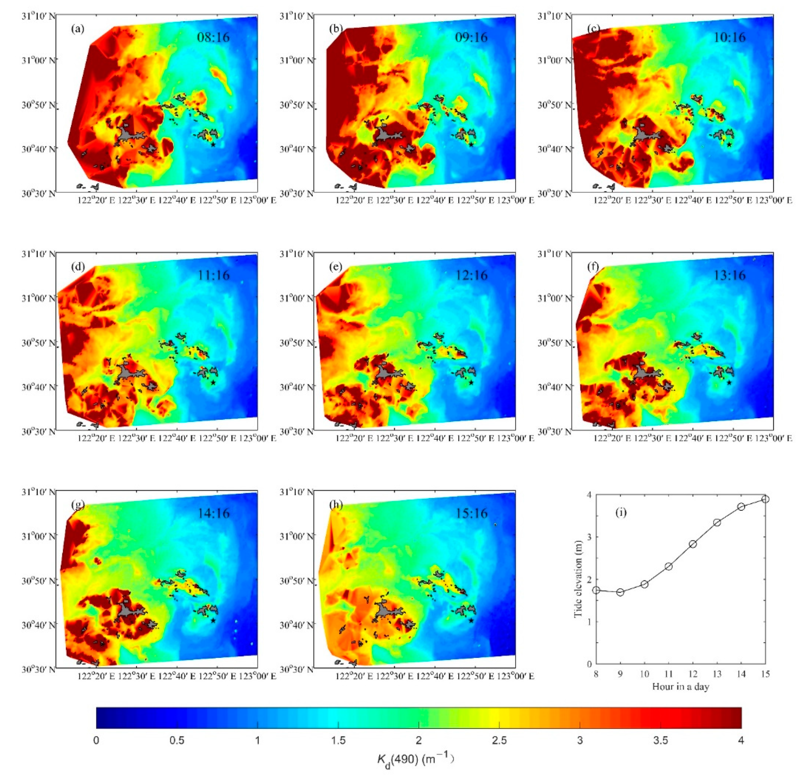
4.2. Application of NDRA to GICI Imagery

To obtain the diurnal variabilities of K d ( 490 ) distribution in the entire high frequency red tide area, GOCI images from 12 October 2013 were used to retrieve the spatial distribution of K d ( 490 ) based on NDRA. The results at eight moments from 8:00 to 15:00 BJT are shown in Figure 13a–h. The results demonstrate that GOCI images can provide reasonable real-time monitoring of K d ( 490 ) in the transition area out of the Yangtze Estuary. The value of K d ( 490 ) decreases with the increase in the distance from the shore, which is consistent with the spatial distribution of SPM in this area. Additionally, it also confirms the dominant role of SPM on the bio-optical properties of the water column. The tide elevation during this period is shown in Figure 13i. It can be observed that, during this flood tide, high K d ( 490 ) spreads from east to west. The site of the moored optical buoy is marked as a black pentacle (Figure 13a–h), and the K d ( 490 ) variations relative to the fixed location can be investigated clearly. This result shows that K d ( 490 ) decreases during flood tide in the target area, which is also consistent with the results obtained by Liu X.M. et al. [11] in the Yangtze Estuary region.

4.3. Dynamic Factors Affecting K d ( 490 ) Diurnal Variations

4.3.1. Hourly Variations

As demonstrated in Section 3.4, K d ( 490 ) presented complicated diurnal variations during the buoy observation period. The first diurnal variation pattern is typical, which agrees with the single regular correlation between K d ( 490 ) and tide elevation corroborated in another similar study in the Yangtze estuary [11]. This can be considered the result of water body dilution by offshore clear water during flood tide and water body pollution by nearshore turbid water during ebb tide. The 1–2 h delay on the K d ( 490 ) minimum may be due to sediment resuspension induced by tide and to needed sedimentation time, as well as the asymmetry of the M2 tide type in the target area [10,11]. Compared to the first pattern, some “abnormalities” appeared in the second pattern, which may be attributed to other environmental factors, such as wind. The third variation pattern is similar to that of Case-1 water [45], the diurnal changes of which were not significant. It should be caused by the low concentrations of SPM, which is the most susceptible constituent to tide and other dynamic processes. The formation mechanism of the fourth variation pattern cannot be understood intuitively because, in this pattern, the relationship between K d ( 490 ) and tide elevation is positive first, and then changes to negative. Clearly, the variation patterns of K d ( 490 ) in the transition area out of the Yangtze Estuary are more complex than those in the maximum turbidity zone of the Yangtze Estuary [11]. Presumably because, in the latter case, the bio-optical properties are consistently dominated by SPM, while, in the former case, the dominant constituent of the water column keeps changing.
The observed irregular diurnal variations of K d ( 490 ) should be the result of biological effects coupled with various physical factors. In Section 2.1, we have already mentioned that the hydrological context of our target area is regulated by multiple factors. In particular, the effects of tide, wind, rainfall, and water mass on K d ( 490 ) diurnal variations are discussed in this section. K d ( 490 ) is plotted against tide elevation, wind speed, wind direction, rainfall, salinity and temperature. The results from linear regressions between K d ( 490 ) at each moment, and the corresponding wind speed, wind direction, tide elevation, and accumulated rainfall of the previous hour, were all not statistically significant ( R 2 < 0.1). By considering the lag influence of wind and tide, the relationships between K d ( 490 ) and the wind speed, wind direction, and tide elevation (1, 2 and 3 h before the K d ( 490 ) measurement) were further investigated. However, no statistically significant results were obtained. R 2 from linear regression between K d ( 490 ) and the corresponding seawater temperature was 0.13, and these two quantities were negatively correlated. R 2 from linear regression between K d ( 490 ) and salinity was not statistically significant ( R 2 = 0.006). In addition, the effects of multiple hydrometeorological factors on the diurnal variation of K d ( 490 ) in the four types of variation patterns were researched alone. The linear-regression results were similar to all 43 days discussed together.
The linear regression between K d ( 490 ) and tide range was further studied. It was found that there was no apparent relationship between K d ( 490 ) and the tide range from one to several hours before K d ( 490 ) measurements. However, when the 43 groups of data were divided into autumn (from 1 September to 31 October) and winter (from 1 November to 31 January) data, relatively significant correlations between the mean K d ( 490 ) in a flood/ebb tide and the corresponding tide ranges (Figure 14a,b) were observed. K d ( 490 ) increases as the tide ranges increases. R 2 from linear regression between the tide range and K d ( 490 ) is 0.14/0.21 for the autumn flood/ebb tide; meanwhile, for winter, R 2 from linear regression between the tide range and K d ( 490 ) is 0.73/0.36 for the flood/ebb tide. Thus, it is demonstrated that tide range is the most influential factor and the dominant effect of tide in the target area is enhancing local sediment resuspension (reflected by tide range). Combining the correlation of K d ( 490 ) with tide elevation in the first and second patterns, we think that the role of tide motion on the horizontal transportation of SPM from the ambient sea (reflected by tide elevation) is not negligible, but secondary to the local sediment resuspension effect.

4.3.2. Daily Variation

The influences of several hydrometeorological factors on K d ( 490 ) during a spring–neap tide cycle were researched. Linear regressions were performed between the daily average of K d ( 490 ) and the corresponding daily average of wind speed, wind direction, tide height, salinity, and temperature, and daily accumulated total rainfall. The daily mean K d ( 490 ) was plotted against all the factors mentioned above, with a lag of zero and one day, respectively (Figure 15a,b). The R 2 s from the linear regressions are also shown in Figure 15. When no lag was considered, significant positive correlations were found between K d ( 490 ) and the wind speed, wind direction, total rainfall, and salinity, the R 2 s of which are 0.71, 0.49, 0.17, and 0.39, respectively. However, there was no apparent relations between K d ( 490 ) and tide elevation, as well as temperature. Taking the hysteresis of each factor into account, a one-day lag was considered. Consequently, R 2 from linear regression between K d ( 490 ) and wind speed decreased from 0.71 to 0.26, while the R 2 between K d ( 490 ) and salinity increased from 0.39 to 0.68. R 2 s from linear regression between K d ( 490 ) and wind direction as well as the total rainfall became insignificant, with R 2 values of 0.04 and 0.02, respectively.
When the wind speed increases, the value of K d ( 490 ) becomes larger because wind can initiate the resuspension of sediments from the lower water layer and enhance the vertical mixing of the entire water column, increasing SPM in the upper water layers [46,47]. As demonstrated in a previous study, the seasonal sediment plume out the Yangtze Estuary can extend to the vicinity of 122°40′E outside the south slot of the Yangtze Estuary during our observation [48], which is close to the position of our buoy (122°49′E, 30°40.7′N). The sediment plume was driven by the cooling of the upper ocean and enhanced surface winds during the fall and winter seasons [9]. The theories for the occurrence of sediment plume in autumn and winter are consistent with the phenomenon that K d ( 490 ) is correlated with wind speed to a certain degree in our target area. In theory, when the south wind is dominant, turbid water with a high SPM from the largest turbid zone should be transported to our target area by wind waves. However, K d ( 490 ) and the wind direction are negatively correlated here, which indicates that the influence of wind on the suspended sediment transportation is small.
R 2 from linear regression between K d ( 490 ) and tide elevation was found to be insignificant. However, from the general trend in the entire spring–neap tide cycle, it can be seen that K d ( 490 ) is larger, and its diurnal variation is more significant during spring than during neap. Moreover, as described in Section 4.2, when the data were classified into flood and ebb data (from 20 September to 5 October), R 2 from linear regression between K d ( 490 ) and tide range can be greater than 0.1 (Figure 14a). The horizontal transportation of SPM from the ambient sea and the enhancement of the local SPM resuspension caused by the tide current are stronger during spring tide. Therefore, the impact of the tide transforming from spring to neap tide is significant.
K d ( 490 ) increases as the aggregated rainfall over the target area increases. It can be speculated that the rainfall mainly increases runoff from the adjacent islands, resulting in high loads of sediments and CDOM, while its dilution effect on seawater is relatively weak. In particular, a high value of R 2 from linear regression between K d ( 490 ) and salinity was obtained. By integrating low linear-regression R 2 (< 0.1) between K d ( 490 ) and temperature, it can be inferred that the prevailing upwelling along the coast of the East China Sea did not exert a significant influence on the upper-layer water in our target area, and the reason for the correlation between K d ( 490 ) and salinity needs to be investigated further, for their positive relationship.

5. Conclusions

In this study, based on the field optical buoy dataset, we evaluated the accuracy of the GOCI L2 K d ( 490 ) , as well as the performances of six empirical algorithms for the estimation of K d ( 490 ) in the coastal East China Sea. Our results show alarge uncertainty for GOCI L2 K d ( 490 ) by comparation between GOCI L2 K d ( 490 ) and buoy-measured K 12 ( 490 ) , with the MAPE and RMSE at 69.57%, and 0.70 m−1, respectively. Similarly, the MAPE and RMSE between GOCI L2 K d ( 490 ) and buoy-measured K 13 ( 490 ) were 68.86%, and 0.71 m−1, respectively. NDRA performed best among the six examined algorithms, with MAPE and RMSE reaching 0.29 m−1 and 27.31%, respectively. We studied the diurnal variations of K d ( 490 ) in the coastal East China Sea based on buoy data. Four main types of K d ( 490 ) diurnal variation were found, showing more complex variation properties than in the areas closer to shore. GOCI images were also used to observe the distribution of K d ( 490 ) at eight moments in a day for a high-frequency red tide area. K d ( 490 ) decreased at flood tide and increased at ebb tide. In addition, we also analyzed the influences of several hydrometeorological factors on the diurnal variation of K d ( 490 ) . The results show that tide has the greatest effect, whereas the disturbance from wind is temporary. In particular, these dynamic processes mainly affect K d ( 490 ) by interfering with the resuspension of sediment, and their effect on sediment transport is secondary.

Author Contributions

Conceptualization, Y.Z. (Yu Zhang), Z.X. and G.W.; methodology, Y.Z. (Yu Zhang), Z.X. and G.W.; software, Y.Z. (Yu Zhang), W.Z. (Wendi Zheng), L.D., Y.Z. (Yinxue Zhang); investigation, Y.Y., Z.X., K.Z.; resources, Y.Y., Y.L.; writing—original draft preparation, Y.Z. (Yu Zhang).; writing—review and editing, Y.Z. (Yu Zhang); visualization, Y.Z. (Yu Zhang); supervision, Z.X., Y.Y.; project administration, Y.Y.; funding acquisition, Z.X., Y.Y., W.C. and W.Z. (Wen Zhou). All authors have read and agreed to the published version of the manuscript.

Funding

This study was funded by the National Science & Technology Fundamental Resources Investigation Program of China (2018FY100100); the Key Special Project for Introduced Talents Team of Southern Marine Science and Engineering Guangdong Laboratory (Guangzhou) (GML2019ZD0602); the National Natural Science Foundation of China (NSFC) (42076190, 41776044); the Key Deployment Project of Centre for Ocean Mega-Research of Science, Chinese academy of science (COMS2019J10); Special Project for Marine Economic Development (Six Major Marine Industries) of Guangdong Province (GDNRC2020019), and the Guangdong Key Laboratory of Ocean Remote Sensing (2017B030301005).

Acknowledgments

We are indebted to NASA and KOSC for providing GOCI data. We also express our appreciations to colleagues in the Optics Laboratory at the South China Sea Institute of Oceanology, Chinese Academy of Sciences, who contributed to the design and deployment of the optical buoy used in this study.

Conflicts of Interest

The authors declare no conflict of interest.

References

  1. Cahoon, L.B.; Beretich, G.R.; Thomas, C.J.; McDonald, A.M. Benthic microalgal production at Stellwagen Bank, Massachusetts Bay, USA. Mar. Ecol. Prog. Ser. 1993, 102, 179–185. [Google Scholar] [CrossRef]
  2. IOCCG. Remote Sensing of Ocean Colour in Coastal, and Other Optically-Complex, Waters; IOCCG: Dartmouth, NS, Canada, 2000. [Google Scholar]
  3. Lee, Z.; Weidemann, A.; Kindle, J.; Arnone, R.; Carder, K.L.; Davis, C. Euphotic zone depth: Its derivation and implication to ocean-color remote sensing. J. Geophys. Res. Ocean. 2007, 112, 11. [Google Scholar] [CrossRef] [Green Version]
  4. Li, G.; Ping, G.; Fang, W.; Qiang, L. Estimation of ocean primary productivity and its spatio-temporal variation mechanism for East China Sea based on VGPM model. J. Geogr. Sci. 2004, 14, 32–40. [Google Scholar] [CrossRef]
  5. Majozi, N.P.; Salama, M.S.; Bernard, S.; Harper, D.M.; Habte, M.G. Remote sensing of euphotic depth in shallow tropical inland waters of Lake Naivasha using MERIS data. Remote Sens. Environ. 2014, 148, 178–189. [Google Scholar] [CrossRef]
  6. Jerlov, N.G. CLASSIFICATION OF SEA-WATER IN TERMS OF QUANTA IRRADIANCE. J. Mar. Sci. 1977, 37, 281–287. [Google Scholar] [CrossRef]
  7. Saulquin, B.; Hamdi, A.; Gohin, F.; Populus, J.; Mangin, A.; d’Andon, O.F. Estimation of the diffuse attenuation coefficient KdPAR using MERIS and application to seabed habitat mapping. Remote Sens. Environ. 2013, 128, 224–233. [Google Scholar] [CrossRef] [Green Version]
  8. Son, S.; Wang, M.H. Water properties in Chesapeake Bay from MODIS-Aqua measurements. Remote Sens. Environ. 2012, 123, 163–174. [Google Scholar] [CrossRef] [Green Version]
  9. Shi, W.S.; Wang, M.H. Satellite observations of the seasonal sediment plume in central East China Sea. J. Mar. Syst. 2010, 82, 280–285. [Google Scholar] [CrossRef]
  10. Shi, W.; Wang, M.H.; Jiang, L.D. Spring-neap tidal effects on satellite ocean color observations in the Bohai Sea, Yellow Sea, and East China Sea. J. Geophys. Res. Ocean. 2011, 116, 13. [Google Scholar] [CrossRef]
  11. Liu, X.M.; Wang, M.H. Analysis of ocean diurnal variations from the Korean Geostationary Ocean Color Imager measurements using the DINEOF method. Estuar. Coast. Shelf Sci. 2016, 180, 230–241. [Google Scholar] [CrossRef]
  12. Wang, M.H.; Ahn, J.H.; Jiang, L.D.; Shi, W.; Son, S.; Park, Y.J.; Ryu, J.H. Ocean color products from the Korean Geostationary Ocean Color Imager (GOCI). Opt. Express 2013, 21, 3835–3849. [Google Scholar] [CrossRef] [PubMed]
  13. Yu, X.L.; Salama, M.S.; Shen, F.; Verhoef, W. Retrieval of the diffuse attenuation coefficient from GOCI images using the 2SeaColor model: A case study in the Yangtze Estuary. Remote Sens. Environ. 2016, 175, 109–119. [Google Scholar] [CrossRef] [Green Version]
  14. Tiwari, S.P.; Shanmugam, P. A Robust Algorithm to Determine Diffuse Attenuation Coefficient of Downwelling Irradiance From Satellite Data in Coastal Oceanic Waters. IEEE J. Sel. Top. Appl. Earth Obs. Remote Sens. 2014, 7, 1616–1622. [Google Scholar] [CrossRef]
  15. Wang, J.H.; Wu, J.Y. Occurrence and potential risks of harmful algal blooms in the East China Sea. Sci. Total Environ. 2009, 407, 4012–4021. [Google Scholar] [CrossRef] [PubMed]
  16. Zhang, T.; Fell, F. An empirical algorithm for determining the diffuse attenuation coefficient Kd in clear and turbid waters from spectral remote sensing reflectance. Limnol. Oceanogr. Methods 2007, 5, 457–462. [Google Scholar] [CrossRef]
  17. Cui, T.; Cao, W.; Jie, Z.; Hao, Y.; Yu, Y.; Zu, T.; Wang, D. Diurnal variability of ocean optical properties during a coastal algal bloom: Implications for ocean colour remote sensing. Int. J. Remote Sens. 2013, 34, 8301–8318. [Google Scholar] [CrossRef]
  18. Zhao, J.; Cao, W.X.; Xu, Z.T.; Ai, B.; Yang, Y.Z.; Jin, G.Z.; Wang, G.F.; Zhou, W.; Chen, Y.; Chen, H.Y.; et al. Estimating CDOM Concentration in Highly Turbid Estuarine Coastal Waters. J. Geophys. Res. Oceans 2018, 123, 5856–5873. [Google Scholar] [CrossRef]
  19. Zhao, J.; Cao, W.X.; Xu, Z.T.; Ye, H.B.; Yang, Y.Z.; Wang, G.F.; Zhou, W.; Sun, Z.H. Estimation of suspended particulate matter in turbid coastal waters: Application to hyperspectral satellite imagery. Opt. Express 2018, 26, 10476–10493. [Google Scholar] [CrossRef] [PubMed]
  20. Mao, Z.H.; Chen, J.Y.; Pan, D.L.; Tao, B.Y.; Zhu, Q.K. A regional remote sensing algorithm for total suspended matter in the East China Sea. Remote Sens. Environ. 2012, 124, 819–831. [Google Scholar] [CrossRef]
  21. Shi, J.Z. Tidal resuspension and transport processes of fine sediment within the river plume in the partially-mixed Changjiang River estuary, China: A personal perspective. Geomorphology 2010, 121, 133–151. [Google Scholar] [CrossRef]
  22. Zhou, M.J.; Shen, Z.L.; Yu, R.C. Responses of a coastal phytoplankton community to increased nutrient input from the Changjiang (Yangtze) River. Cont. Shelf Res. 2008, 28, 1483–1489. [Google Scholar] [CrossRef]
  23. Lu, M.; Zhu, Y. Whether and Cliamate characteristics of the Coastal Gale in Zhejiang. J. Hangzhou Norm. Univ. Nat. Sci. Ed. 2011, 10, 474–480. [Google Scholar]
  24. Liu, J.P.; Li, A.C.; Xu, K.H.; Veiozzi, D.M.; Yang, Z.S.; Milliman, J.D.; DeMaster, D. Sedimentary features of the Yangtze River-derived along-shelf clinoform deposit in the East China Sea. Cont. Shelf Res. 2006, 26, 2141–2156. [Google Scholar] [CrossRef]
  25. Shang, D.H.; Xu, H.P. Qualitative Dynamics of Suspended Particulate Matter in the Changjiang Estuary from Geostationary Ocean Color Images: An Empirical, Regional Modeling Approach. Sensors 2018, 18, 4186. [Google Scholar] [CrossRef] [Green Version]
  26. Bai, X.; Yang, Y.; Zhou, L.; Ren, S.; Liu, D.; Liu, Z.; Wang, Z. Variations in Shell Frame Characteristic among Three Species of Mytilus in Shengsi Waters of the East China Sea. Oceanol. Limnol. Sin. 2014, 45, 1078–1084. [Google Scholar]
  27. Austin, R.W. The Remote Sensing of Spectral Radiance from Below the Ocean Surface; Optical Aspects of Oceanography; Academic Press: London, UK; New York, NY, USA, 1974; Volume 14. [Google Scholar]
  28. Huang, X.C.; Zhu, J.H.; Han, B.; Jamet, C.; Tian, Z.; Zhao, Y.L.; Li, J.; Li, T.J. Evaluation of Four Atmospheric Correction Algorithms for GOCI Images over the Yellow Sea. Remote Sens. 2019, 11, 27. [Google Scholar] [CrossRef] [Green Version]
  29. Bailey, S.W.; Werdell, P.J. A multi-sensor approach for the on-orbit validation of ocean color satellite data products. Remote Sens. Environ. 2006, 102, 12–23. [Google Scholar] [CrossRef]
  30. Choi, J.K.; Park, Y.J.; Ahn, J.H.; Lim, H.S.; Eom, J.; Ryu, J.H. GOCI, the world’s first geostationary ocean color observation satellite, for the monitoring of temporal variability in coastal water turbidity. J. Geophys. Res. Ocean. 2012, 117, 10. [Google Scholar] [CrossRef]
  31. Moon, J.E.; Park, Y.J.; Ryu, J.H.; Choi, J.K.; Ahn, J.H.; Min, J.E.; Son, Y.B.; Lee, S.J.; Han, H.J.; Ahn, Y.H. Initial Validation of GOCI Water Products against in situ Data Collected around Korean Peninsula for 2010–2011. Ocean Sci. J. 2012, 47, 261–277. [Google Scholar] [CrossRef]
  32. Ruddick, K.G.; Voss, K.; Boss, E.; Castagna, A.; Frouin, R.; Gilerson, A.; Hieronymi, M.; Johnson, B.C.; Kuusk, J.; Lee, Z.; et al. A Review of Protocols for Fiducial Reference Measurements of Water-Leaving Radiance for Validation of Satellite Remote-Sensing Data over Water. Remote Sens. 2019, 11, 38. [Google Scholar]
  33. Zaneveld, J.R.V.; Boss, E.; Barnard, A. Influence of Surface Waves on Measured and Modeled Irradiance Profiles. Appl. Opt. 2001, 40, 1442–1449. [Google Scholar] [CrossRef] [PubMed]
  34. Cao, W.; Yang, Y.; Zhang, J.; Ke, T.; Lu, G.; Li, C.; Guo, C.; Sun, Z. Design and test of moored optical buoy. J. Trop. Oceanogr. 2010, 29, 1–6. [Google Scholar]
  35. Yang, Y.; Cao, W.; Sun, Z.; Wang, G.F. Development of Real-Time Hyperspectral Radiation Sea-Observation System. Acta Opt. Sin. 2009, 29, 102–107. [Google Scholar] [CrossRef]
  36. Yang, Y.; Sun, Z.; Cao, W.X.; Li, C.; Zhao, J.; Zhou, W.; Lu, G.; Ke, T.; Guo, C. Design and Experimentation of Marine Optical Buoy. Spectrosc. Spectr. Anal. 2009, 29, 565–569. [Google Scholar]
  37. Zhang, Y.; Wang, G.; Xu, Z.; Yang, Y.; Zhou, W.; Zheng, W.; Zeng, K.; Deng, L. Retrieval of diffuse attenuation coefficient in high frequency red tide area of the East China Sea based on buoy observation. J. Trop. Oceanogr. 2020, 39, 71–83. [Google Scholar]
  38. Voss, K.J.; Flora, S. Spectral Dependence of the Seawater-Air Radiance Transmission Coefficient. J. Atmos. Ocean. Technol. 2017, 34, 1203–1205. [Google Scholar] [CrossRef]
  39. Wang, X.M.; Tang, J.W.; Ding, J.; Ma, C.F.; Li, T.J.; Wang, X.Y.; Bi, D.Y. The retrieval algorithms of diffuse attenuation and transparency for the case-II waters of the Huanghai Sea and the East China Sea. Acta Oceanol. Sin. 2005, 27, 5. [Google Scholar]
  40. Chen, Y.; Shen, F. Diffuse attenuation coefficient of remote sensing inversion in Yangtze River Estuary’s adjacent sea area in winter. Trans. Oceanol. Limnol. 2014, 4, 27–34. [Google Scholar]
  41. Wang, M.H.; Son, S.; Harding, L.W. Retrieval of diffuse attenuation coefficient in the Chesapeake Bay and turbid ocean regions for satellite ocean color applications. J. Geophys. Res. Ocean. 2009, 114. [Google Scholar] [CrossRef]
  42. Kim, W.; Moon, J.E.; Park, Y.J.; Ishizaka, J. Evaluation of chlorophyll retrievals from Geostationary Ocean Color Imager (GOCI) for the North-East Asian region. Remote Sens. Environ. 2016, 184, 482–495. [Google Scholar] [CrossRef]
  43. Zhao, J.; Barnes, B.; Melo, N.; English, D.; Lapointe, B.; Muller-Karger, F.; Schaeffer, B.; Hu, C.M. Assessment of satellite-derived diffuse attenuation coefficients and euphotic depths in south Florida coastal waters. Remote Sens. Environ. 2013, 131, 38–50. [Google Scholar] [CrossRef]
  44. Melin, F.; Zibordi, G.; Berthon, J.F. Assessment of satellite ocean color products at a coastal site. Remote Sens. Environ. 2007, 110, 192–215. [Google Scholar] [CrossRef]
  45. Concha, J.; Mannino, A.; Franz, B.; Kim, W. Uncertainties in the Geostationary Ocean Color Imager (GOCI) Remote Sensing Reflectance for Assessing Diurnal Variability of Biogeochemical Processes. Remote Sens. 2019, 11, 295. [Google Scholar] [CrossRef] [Green Version]
  46. Chen, S. Seasonal, neap-spring variation of sediment concentration in the joint area between Yangtze Estuary and Hangzhou Bay. Sci. China 2001, 44, 57–62. [Google Scholar] [CrossRef]
  47. Zuo, S.H.; Zhang, N.C.; Bei, L.I.; Chen, S.L. A study of suspended sediment concentration in Yangshan deep-water port in Shanghai, China. Int. J. Sediment Res. 2012, 27, 50–60. [Google Scholar] [CrossRef]
  48. Cao, P.; Yan, S. Suspended Sediments front and its Impacts on the Materials Transport of the Changjiang Estuary. J. East. China Norm. Univ. Nat. Sci. 1996, 1, 85–94. [Google Scholar]
Figure 1. Locations of the optical buoy, Shengsi meteorological station, and Lv Huashan tide gauge station, with isobaths (units of meters) of the surrounding continental shelves. The black rectangle indicates the approximate range of a high-frequency red tide area out of the Yangtze Estuary [22].
Remotesensing 13 01676 g001
Figure 2. The optical buoy used in this study. (a) Photograph of the buoy in operation. (b) Schematic of the structure of the buoy.
Remotesensing 13 01676 g002
Figure 3. The coefficients of variation of depth and K d ( 490 ) at the adjacent time of data acquisition (redrawn from Zhang et al. [37]).
Remotesensing 13 01676 g003
Figure 4. Linear correlations between buoy-measured K d 12 ( 490 ) and K d 13 ( 490 ) (redrawn from Zhang et al. [37]).
Remotesensing 13 01676 g004
Figure 5. Histogram and cumulative percentage for buoy-measured K d 12 ( 490 ) .
Remotesensing 13 01676 g005
Figure 6. Comparisons between GOCI L2 K d ( 490 ) and buoy-measured K d 12 ( 490 ) , as well as K d 13 ( 490 ) .
Remotesensing 13 01676 g006
Figure 7. In situ buoy K d 12 ( 490 ) versus derived K d ( 490 ) for (a) the Wang X.M. algorithm, (b) Chen algorithm, (c) Wang M.H. algorithm, (d) Zhang algorithm, (e) Tiwari algorithm and (f) NDRA, applied to validation datasets.
Remotesensing 13 01676 g007
Figure 8. K d ( 490 ) newly derived from GOCI L2 R rs by NDRA.
Remotesensing 13 01676 g008
Figure 9. Diurnal variation of K d ( 490 ) and tide elevation for the 12 days from 08:00 to 17:00 BJT: (a) 5 October 2013; (b) 22 October 2013; (c) 5 November 2013; (d) 22 September 2013; (e) 26 September 2013; (f) 8 November 2013; (g) 27 September 2013; (h) 28 September 2013; (i) 29 September 2013; (j) 28 October 2013; (k) 29 October 2013; (l) 29 November 2013.
Remotesensing 13 01676 g009
Figure 10. Diurnal variation of buoy K d ( 490 ) and the corresponding meteorological parameters in the spring–neap cycle between 20 September and 5 October, 2013. (a) Time series of hourly K d ( 490 ) and tide elevation. (bd) Daily accumulated rainfall, daily mean wind direction, and velocity, respectively. The rainfall, wind direction, and wind velocity were calculated from data from 00:00 to 23:00 BJT.
Remotesensing 13 01676 g010
Figure 11. Comparison of R rs ( λ ) spectra between GOCI L2 estimations and buoy measurements at 412, 443, 490, 555, 660 and 680 nm. Note that Buoy12 and Buoy13 represent R rs of the water column between the first and second, and first and third radiometers, respectively.
Remotesensing 13 01676 g011
Figure 12. GOCI R rs versus buoy R rs 12 at bands of 412, 443, 490, 555, 660, and 680 nm. The black solid line refers to the 1:1 line.
Remotesensing 13 01676 g012
Figure 13. Hourly maps of K d ( 490 ) in the target high-frequency red tide area retrieved from the GOCI images on 12 October 2013. The labeled time in the image corresponds to the observation time in BJT. The black pentacle refers to the site of the moored optical buoy. The last sub-plot shows the synchronous hourly tide elevation observed from Lv Huashan tide gauge station.
Remotesensing 13 01676 g013
Figure 14. Relations between the mean value of K d ( 490 ) and tide range of a flood or an ebb tide in different seasons. (a) Data for autumn (from 20 September to 5 October) and (b) data for winter (from 8 November to 11 January).
Remotesensing 13 01676 g014
Figure 15. Correlations between daily mean K d ( 490 ) and daily mean wind speed (black), wind direction (red), tide height (blue), accumulated rainfall (pink), salinity (green), as well as temperature (orange). The panels (a,b) illustrate the relationships with a lag of 0 day and 1 day, respectively. The R 2 s from the linear regressions between K d ( 490 ) and different parameters are annotated.
Remotesensing 13 01676 g015
Table 1. Different algorithms of K d 12 ( 490 ) adjusted for the central wavelengths of the GOCI.
IDAlgorithm
Wang X.M. [39]
K d ( 490 ) = 10 { 0.581 R rs ( 490 ) R rs ( 555 ) + 1.3916 [ R rs ( 660 ) + R rs ( 555 ) ] + 0.299 }
Chen [40]
K d ( 490 ) = 10 [ 0.0357 R rs ( 555 ) R rs ( 490 ) + 0.8218 R rs ( 660 ) R rs ( 490 )     0.3495 ]
Wang M.H. [41]
K d ( 490 ) = 1.146   ×   10 5 R rs ( 490 ) + 2.0638 R rs ( 660 ) R rs ( 490 ) + 1.1078 [ 0.3113 R rs ( 660 )     0.1474 ] [ 1     5 e 10 R rs ( 490 )     R rs ( 660 ) R rs ( 490 ) ]
Zhang [16]
R rs ( 490 ) R rs ( 555 ) 0.85 ,   K d ( 490 ) = 10 { 49.26 [ R rs ( 490 ) R rs ( 555 ) ] 3     11.03 [ R rs ( 490 ) R rs ( 555 ) ] 2     2.359 [ R rs ( 490 ) R rs ( 555 ) ]     0.7932 } + 0.016

R rs ( 490 ) R rs ( 555 ) 0.85 ,   K d ( 490 ) = 10 { 1.33 [ R rs ( 490 ) R rs ( 660 ) ] 3     1.668 [ R rs ( 490 ) R rs ( 660 ) ] 2     1.349 [ R rs ( 490 ) R rs ( 660 ) ] + 0.6629 } + 0.016
Tiwari [14]
K d ( 490 ) = 1.8034 R rs ( 660 ) R rs ( 490 ) + 0.2534
NneDRA [37]
K d ( 490 ) = 2.1252 R rs ( 660 ) R rs ( 490 )     0.0999 R rs ( 555 ) R rs ( 490 ) + 0.2916
Table 2. Statistical comparison results between the estimated K d ( 490 ) from different inversion algorithms and buoy-measured K d 12 ( 490 ) .
Algorithm
RMSE   ( m 1 )
MAPE (%)SlopeInterceptR2N
Wang X.M. [39]0.5043.890.150.690.15568
Chen [40]0.4028.870.860.120.60568
Wang M.H. [41]0.4043.650.79−0.110.76568
Zhang [16]0.7849.911.88−0.680.74568
Tiwari [14]0.3028.150.660.320.71568
NDRA [37]0.2927.310.760.240.72568
Table 3. Statistics for the remote sensing reflectance matchup data between the GOCI L2 R rs and buoy-measured R rs 12 .
λ ( m n )
Mean RatioMAPE (%)
RMSE   ( sr 1 )
R 2
SlopeInterceptN
4121.4547.290.00220.600.820.002613
4431.4041.010.00260.770.800.003713
4901.0513.510.00190.810.710.003613
5550.9512.700.00290.800.700.003713
6601.4850.250.00190.850.960.001513
6801.4949.730.00170.850.980.001313
Publisher’s Note: MDPI stays neutral with regard to jurisdictional claims in published maps and institutional affiliations.

