Article

The Penetration Analysis of Airborne Ku-Band Radar Versus Satellite Infrared Lidar Based on the Height and Energy Percentiles in the Boreal Forest

1
Electronic Information School, Wuhan University, Wuhan 430079, China
2
Department of Remote Sensing and Photogrammetry, Finnish Geospatial Research Institute, Geodeetinrinne 2, 02431 Kirkkonummi, Finland
3
Key Laboratory of Intelligent Infrared Perception, Shanghai Institute of Technical Physics, Chinese Academy of Sciences (CAS), Shanghai 200043, China
*
Author to whom correspondence should be addressed.
Remote Sens. 2021, 13(9), 1650; https://doi.org/10.3390/rs13091650
Submission received: 25 March 2021 / Revised: 12 April 2021 / Accepted: 14 April 2021 / Published: 23 April 2021
(This article belongs to the Special Issue New Technologies for Earth Remote Sensing)

Abstract

:
The paper investigates the penetration properties of an airborne Ku-band frequency modulated continuous waveform (FMCW) profiling radar named Tomoradar and a satellite near-infrared lidar into the boreal forest of Finland. We achieve the accumulative energy distributions based on the Tomoradar waveforms and the satellite lidar waveforms generated from the high-density airborne lidar data within Tomoradar footprints. By comparing two groups of the height percentiles and energy percentiles derived from the accumulative energy distributions, we evaluate the relationship of penetrations between the Ku-band microwave and near-infrared laser according to the coefficients of the determination (COD), and the root mean square errors (RMSE) of linear regression analyses. The quantitative analysis results demonstrate that the height and energy percentiles derived from Tomoradar waveforms correlate well with those from satellite lidar waveforms with the mean correlation coefficients of more than 0.78 and 0.85. The linear regression models for the height and energy percentile produce excellent fits with the mean CODs of 0.95 and 0.90 and the mean RMSEs of 1.25 m and 0.03, respectively. Less than 15% of height percentiles and 87.54% of the energy percentiles in the sixth stratum near the ground derived from Tomoradar waveforms surpass those from satellite lidar waveforms. Hence, the Ku-band microwave can penetrate deeper into the forest than the near-infrared laser at the same spatial scale. In addition, quadratic fitting models are established to describe the differences of the height percentile (DHP) and the energy percentile (DEP) to expound the canopy height and closure contributions numerically. The facts that the CODs of the DHP and DEP individually are more than 0.96 and 0.89 and the fitting residual histograms approximate to normal distributions reveal the reliabilities of the proposed fitting models. Thus, the penetration analyses are valid for the explorations on the FMCW radar applications and the data fusion of the Ku-band radar and near-infrared lidar in the forest investigations.

Graphical Abstract

1. Introduction

As crucial ecosystems, forests play prominent roles in determining carbon storage, climate and ecological functionalities [1,2]. Monitoring the forest structure’s spatial and temporal characteristics contributes to understanding carbon stock modelling and global environmental changes [3,4].
Remote sensing technologies have been proved to be highly effective for acquiring more accurate and spatially continuous forest structure properties on a large scale in a rapid manner. Passive optical imaging systems can only collect the reflected sunlight from the exterior canopy surface and are incapable of obtaining the vertical forest structures inside the canopy [5,6]. However, active remote sensing devices, including lidar and radar systems, can explore the understory vegetation and the ground to become the primary technologies in forest investigation.
Full waveform, small-footprint lidar and large footprint satellite lidar transmit laser pulses into the forest and record the vegetation and ground returns. Combing with the navigation and positioning information of the platforms, the lidar systems are valuable for estimating various forest inventory parameters, including canopy height, leaf area index and biomass [7,8,9,10]. Synthetic aperture radar (SAR) has been well developed in past decades worldwide and employed to extract the canopy height and stem volume [11,12], but the vertical canopy structure information is still missing due to poor penetration. To resolve such a penetration problem and as a complement to SAR and lidar, a light-weighted Ku-band frequency-modulated continuous waveform (FMCW) profiling radar aboard an airborne platform, named Tomoradar, was designed by the Finnish Geospatial Research Institute to collect the full polarisation backscattered signals from the forest in Finland [13]. A wide range of forest parameters, including ground level, canopy top elevation, canopy height and leaf area index, are retrieved by processing the Tomoradar waveforms [14,15,16]. However, some disparities in these forest parameters are derived from lidar data and Tomoradar waveforms because of the varying signal propagation and penetration into the forest.
The remote sensing devices’ abilities to measure the canopy structure are strongly dependent on the penetration of the electromagnetic (EM) wavelengths [17]. Near-infrared lidar is bound to present the discrepancies of the penetration with Ku-band Tomoradar. Lidar penetrations were usually investigated by energy penetration index or ground return percentage (the ratio between ground energy and total waveform energy) and the crown’s depth [18,19,20]. Ku-band Tomoradar penetration was analysed according to the backscattered ratio of canopy energy to total waveform energy [21]. However, this research only depicted the energy ratio from the ground or the canopy, and did not present the waveforms’ penetration process through the forest. Moreover, there are very few comparisons that have been implemented concerning lidar and radar penetrations into the forests at the same time and same place.
In this research, benefiting from the cooperative observation of lidar and Tomoradar on the same platform, the penetration properties of the Ku-band microwave and near-infrared laser are explored in Tomoradar waveforms and satellite lidar waveforms simulated from airborne lidar data at the same spatial scale. By processing Tomoradar waveforms and simulating the satellite lidar waveforms, the accumulative energy distributions are derived to generate the two groups of height and energy percentiles (HEP). We provide the comparisons and regression analyses of the HEPs derived from Tomoradar and satellite lidar to expound on these two wavelengths’ penetrations in the boreal forest environment. Two specific objectives are to (1) investigate the quantitative relationships of the HEPs to demonstrate the penetration differences of the Ku-band microwave and near-infrared laser; (2) establish the regression models of the differences of the HEP as functions of the canopy height and closure to present the influence of the canopy structure on the penetration.
The rest of this paper is organised as follows: Section 2 describes the study area, Tomoradar waveforms, lidar data, and illustrates the methods of derivation and comparisons of the HEPs; Section 3 expounds on the results of the HEPs; Section 4 discusses the and regression analyses; finally, the conclusions are drawn in Section 4.

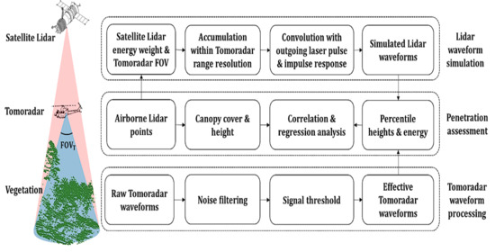
2. Materials and Methods

2.1. Study Area

The study area was located at a fraction of the boreal forest region in Evo, southern Finland (61.19°N, 25.11°E). It was a popular recreation area and consisted of Scots pine, Norway spruce, and birch with different vegetation densities and tree height. Both the Tomoradar and Velodyne VLP-16 laser scanner were mounted on a Bell 206 helicopter with a flight height of 60–100 m to synchronously gather the backscattered waveforms and point clouds of the vegetation and ground in September 2016. There were 41 stripes over the study area with a total length of about 24 km. The flying trajectory of the helicopter during the Tomoradar campaigns is presented in Figure 1. In this study, 17 stripes of Tomoradar waveforms and lidar points are randomly chosen to investigate the penetration of the Ku-band microwave and near-infrared laser.

2.2. Tomoradar Waveforms

The FMCW Tomoradar recorded the backscattered signals from the canopy surface and the underlying ground within the Tomoradar footprint and converted them into waveforms. The effective field of view (FOV) of Tomoradar was 8 degrees, in which the fraction of total radiation energy was supposed to be 91% [22]. Raw Tomoradar waveforms represented the vertical distribution of the Ku-band microwave radiation along the beam path. The Tomoradar system has a range resolution of 15 centimetres and an along-track spatial interval of about 6 centimetres on the ground. Due to a severe intersection of the contiguous footprint in such intervals, we resample the footprint according to the 2-m along-track resolution. Hence, only 5321 Tomoradar waveforms were preserved to be investigated in this study.

2.3. Airborne Lidar Data

The airborne lidar data were acquired by a Velodyne VLP-16 lidar installed on the same platform as the Tomoradar. The instrument instantaneously provided 16 parallel scan lines with a 30° along-track scan angle and only collected the first and strongest returns. The average lidar point density was approximately 36 points per square meter. The high-density airborne lidar data were the representatives of the 3D distributions of vegetation and ground over the study area as references for simulating the satellite lidar waveforms. In addition, the airborne lidar data were filtered to separate the ground and canopy, then the canopy height and closure can be derived in terms of the distance from the ground to canopy top, and the ratio of ground returns to total returns within the Tomoradar FOV, respectively.

2.4. Methods

The penetration of the Ku-band microwave and near-infrared laser into the forest can be directly investigated according to the distributions of Tomoradar waveforms and satellite lidar waveforms, which are the functions of the transmitted microwave and laser energy, surface reflectance and scattering, and atmospheric attenuation. In order to retain the influence of vegetation’s distributions and ground on the penetration of waveforms, each waveform should be normalised by its summation. The percentile heights and energies of the normalised waveforms into the forest are explored to demonstrate the penetration of airborne Ku-band radar and satellite near-infrared lidar. The detailed diagram is illustrated in Figure 2, which includes three processing steps: (a) Satellite Lidar waveform simulation; (b) Tomoradar waveform Processing; (c) Penetration assessment.

2.4.1. Simulating Satellite Lidar Waveform

Satellite lidar waveforms can be simulated from airborne lidar data by convoluting the target cross-section with Gaussian weighting functions of outgoing pulse and impulse response. In our simulation, only the lidar points within Tomoradar FOV are effectively acceptable. The laser footprint on the ground is entirely identical to the Tomoradar footprint and assumed to contain about 86.5% of outgoing laser pulse energy. Given the lidar points x i , y i , z i within a Tomoradar FOV, the simulated lidar waveforms can be described as [20]
W l h = i Q β i ρ i 4 I x i , y i f h Q = i | x i , y i , z i FOV T   and   z i h Δ ρ 2
where   h symbolises the target height, β i represents the surface reflectance and is supposed to be constant in this paper, ρ i is the distance from the lidar system to the target, which is approximately invariable since the satellite altitude is much greater than the target height. FOV T is the Tomoradar FOV, Δ ρ is Tomoradar range resolution. I x i , y i represents the spatial intensity distribution of outgoing laser pulse on the ground and f t is the lidar system function which can be treated as the convolution of the outgoing pulse and impulse response of satellite lidar system. They can be expressed as the following
I x i , y i = exp x i x 0 2 + y i y 0 2 2 d 2 f h = exp 2 h 2 c 2 δ 2
where x 0 , y 0 denotes the laser footprint centroid,   c is light speed, d and δ are the footprint radius and time width at the exp 1 2 points of maximal intensity and lidar system function, respectively. The laser footprint radius varies from 5.5 m to 13.5 m according to the helicopter’s flight height over the study area. The time width of the lidar system function is set to 2 nanoseconds. It should be noted that the simulated lidar waveform generated by Equation (1) is relative in the unit.

2.4.2. Processing of Tomoradar Waveform

Raw Tomoradar waveforms comprise effective signals and noises that may negatively affect the extraction of effective signals. Smooth filtering with a weighted factor of normalised Gaussian distribution is performed to remove the noise [15]. The filtered waveforms above a signal threshold are regarded as the effective Tomoradar waveforms. Here, the signal threshold is usually set to 3 times the standard deviation of the noise, which can be resolved using raw waveforms in both edges. Considering that the distributions of the simulated lidar waveform are irrelevant to the target height, the processed Tomoradar waveforms should also be corrected with the fourth power of the heights from the helicopter to the target according to the radar equation as
W r h = h 4 P r h
where, P r h represents the filtered Tomoradar waveforms above the signal threshold.

2.4.3. Assessing Penetration

The normalised waveforms are the distributions of the vegetation and ground sensed by Tomoradar and satellite lidar. In this study, there are two groups of the waveform parameters serving as the metrics of penetration: (a) the 15th, 30th, 45th, 60th, 75th and 90th height percentiles ( H 15 , H 30 ,   H 45 , H 60 ,   H 75 ,   H 90 ); (b) the energy percentiles in six equal height parts ( E 1 ,   E 2 ,   E 3 ,   E 4 , E 5 , E 6 ), as presented in Figure 3.
These height and energy percentiles are calculated from the energy proportions and heights of the normalised waveforms’ accumulative distributions [7,23]. Height percentiles represent the vertical structure distributions of the vegetation within the footprint, and energy percentiles describe the energy levels distributed in different strata of the vegetation. It is expected that the more substantial penetration corresponds to a greater energy percentile in the lowest height and a smaller height percentile in the same energy proportion. We directly compare the height and energy percentiles derived from Tomoradar waveforms and satellite lidar waveforms to demonstrate Ku-band microwave and near-infrared laser penetration.
If we symbolise the height and energy percentiles derived from Tomoradar waveforms and satellite lidar waveforms as ( HP t , EP t ) and ( HP l , EP l ) , the linear regression analyses with a confidence level of 95% are employed in the estimation of the relationship between the height and energy percentiles. The coefficient of determination (COD, r 2 ) and the root mean square error (RMSE, δ r ) can be given by
r H 2 = 1 HP t HP r 2           HP t HP t ¯ 2           ,   δ H r = HP t HP r 2           n 1 .
r E 2 = 1 EP t EP r 2           EP t EP t ¯ 2           ,   δ E r = EP t EP r 2           n 1 .
where HP r represents predicted value of HP t as a function of HP l , and EP r represents predicted value of EP t as a function of EP l with the linear regression models. HP t ¯ and EP t ¯ are the means of   HP t and EP t , respectively, n is the number of Tomoradar measurements in this study. The COD is the proportion of the variance in the dependent variable that is predictable from the independent variables in statistics. The associations of a higher COD and a lower RMSE indicate a better fitting for the predicted model.
In addition, we intend to investigate the influence of the vegetation structure distributions on the penetrations of the Ku-band microwave and near-infrared laser. Considering that the metrics of the canopy height and closure are the representatives of vegetation structure, we would establish the fitting model about the differences of the height and energy percentiles derived from Tomoradar waveforms and satellite lidar waveforms as a function of canopy height and closure. Meanwhile, the contributions of canopy height and closure to the penetration of the Ku-band microwave and near-infrared laser can be quantitatively explored.

3. Results

3.1. The Correlation Analysis of Tomoradar Waveforms and Satellite Lidar Waveforms

If Tomoradar radiation hits a region with a 9.5-m radius where there are multiple trees with 15-m canopy height and 0.57 canopy closure, a visual comparison between Tomoradar waveform and satellite lidar waveform is presented in Figure 4.
Both the Tomoradar waveform and satellite lidar waveform are composed of two components: a vegetation return and a ground return. The composition and 3D structure of the vegetation and the ground determine the waveform distributions. Furthermore, we discover that the Tomoradar waveform shifts towards the ground relative to the satellite lidar waveform. It implies that more Tomoradar radiation energy penetrated inside the canopy rather than that of the laser pulse. Meanwhile, it can be observed that the Tomoradar waveform has a strong correlation with the satellite lidar waveform based on the Pearson’s correlation coefficient of 0.75.
The correlations between Tomoradar waveforms and satellite lidar waveforms are changeable for different scenarios in the study area. We calculate 5321 correlation coefficients and partition them into five segments with a range from 0 to 1 and an interval of 0.2 based on the definition of the correlation strength. By counting the numbers within each segment, we obtain the proportions to 5321 measurements. Hence, we provide the distributions of the correlation coefficients for all measurements and the corresponding proportions, as shown in Figure 5.
The correlation coefficient in Figure 5a is fluctuated for each measurement due to the diversity of the target within the Tomoradar footprint. When the correlation strength varies from very weak to very strong in Figure 5b, the proportions of all measurements rapidly increase and take values of 1.21%, 2.54%, 7.62%, 27.38% and 61.25%, respectively. It means that 88.63% of Tomoradar waveforms correlate very well with satellite lidar waveforms. As such, the Ku-band microwave may have a partially similar penetration feature into the forest with a near-infrared laser at the same spatial scale. Nevertheless, further analysis of these two wavelengths’ penetration should be performed by the following height and energy percentiles.

3.2. The Penetration Analysis Based on the Height and Energy Percentiles

3.2.1. Height Percentile Analysis

According to the method mentioned above for calculating the height percentiles, we obtain the height percentiles derived from Tomoradar waveforms and satellite lidar waveforms (defined as HP t and HP l ) and present the scatterplots and linear regression results of them in Figure 6.
We notice that the height percentiles derived from Tomoradar waveforms correlate well to those from satellite lidar waveforms with a stronger correlation strength of a 0.78 mean correlation coefficient. Moreover, the linear regression models produce an excellent fit with CODs of 0.92–0.99 and RMSEs of 0.07 m–1.99 m. In this case, we may exactly depict the relationship between HP t and HP l using the linear regression models.
Meanwhile, we observe that a single relation of height percentiles derived from Tomoradar waveforms ( HP t ) and satellite lidar waveforms ( HP l ) is expressed as a blue point. Additionally, the majority of these points in Figure 6 locate above the line of Y = X. It implies that the height percentiles of the microwave radar are generally smaller than the height percentiles of lidar. Such a phenomenon means that microwave radar’s penetration capability is more substantial than lidar, which also fits the conclusion of Chen et al., 2017. Furthermore, Table 1 presents three groups of assessment parameters for further investigation.
With the increase in the penetration depth into the forest, the mean and the standard deviation of HP t and HP l decrease rapidly, and HP l gradually approaches to HP t . If the penetrated energy is no more than 45%, the average difference between HP l and HP t is around 3 m. However, when the penetrated energy is equal to 90%, such difference diminishes to 0.65 m. The results suggest that the height percentiles near the canopy top are easily influenced by the wavelength and become more uncertain, but the height percentiles near the ground are less dependent on the wavelength and become more stable. In addition, more than 85% of height percentiles derived from satellite lidar waveforms surpass those from Tomoradar waveforms, which demonstrates that the Ku-band microwave can penetrate deeper into the forest than the near-infrared laser.
To investigate the impact of the structure distributions of the vegetation on the height percentile of HP t and HP l , we illustrate the 3D distributions of the target within the footprint, waveforms and the accumulative energies in three situations: (a) HP t is more considerable than HP l ; (b) HP t is much smaller than HP l ; (c) HP t is approximately equal to HP l , which are presented in Figure 7.
It appears that for a vegetated region with highly dense canopies in Figure 7a, Tomoradar can receive the backscattered signals on the canopy surface and inside the canopy, but satellite lidar only captures the returned signal from the canopy surface. Hence, the canopy return from Tomoradar is more complicated and more significant than that from satellite lidar, which can be employed to retrieve more detailed canopy information. Similarly, for a vegetated region with relatively sparse canopies in Figure 7b, the Ku-band microwave can directly penetrate the ground, but the vegetation’s branches and leaves would reflect laser signals. Thus, the ground return from Tomoradar is higher than that from satellite lidar. For these two situations in Figure 7a,b, the minor variations of the waveform shape heavily influence the distributions of the cumulative energy and result in the enormous differences between the height percentile of HP t and HP l . However, for a flat region without vegetation in Figure 7c, both the Tomoradar waveform and satellite lidar waveform show unimodal characteristics and similar cumulative energy distributions with approximate height percentiles.

3.2.2. Energy Percentile Analysis

Based on the method of resolving the energy percentiles and all 5321 waveforms, we provide the scatterplots and linear regression results of the energy percentiles derived from Tomoradar waveforms and satellite lidar waveforms (defined as EP t and EP l ) as presented in Figure 8.
In Figure 8, the energy percentiles derived from Tomoradar waveforms correlate very well to those from satellite lidar waveforms with an extreme correlation strength of 0.85 mean correlation coefficient. Meanwhile, the linear regression models for the energy percentile produce preferable goodness of fit with the CODs of 0.81–0.99 and the RMSEs of 0.02–0.06. Moreover, the scatter points transfer to the bottom of the line of Y = X with the increase in penetration depth.
We define the proportion of the numbers of EP l EP t to total measurements as γ E , the mean and the standard deviation of EP t and EP l as ( ME t , SE t ) and ( ME l , SE l ), respectively. Their statistical results are enumerated in Table 2. We discover that the maximal differences between ME t and ME l are located in the highest and lowest height strata, demonstrating that the energy percentiles near the canopy top and the ground are more greatly affected by the wavelength. Meanwhile, the proportion γ E decreases rapidly from 91.13% to 12.46% when the waveform penetrates from the first stratum to the sixth stratum. It shows 87.54% of the energy percentiles in the sixth stratum derived from Tomoradar waveforms exceed those from satellite lidar waveforms. The results validate that the Ku-band microwave can more easily reach the ground and has more substantial penetration into the forest than the near-infrared laser.
We explore the influence of the target distributions on the energy percentiles for three situations mentioned in Figure 7 and plot the corresponding energy percentiles EP t and EP l as illustrated in Figure 9.
We observe that, for a vegetated region with highly dense canopies in Figure 7a, the differences between EP l and EP t near the canopy top and the ground are more significant due to the vast variations between the Tomoradar waveform and satellite lidar waveform. Similarly, for a vegetated region with relatively sparse canopies in Figure 7b, the more considerable difference is distributed near the ground. However, for a flat region without vegetation in Figure 7c, the energy percentile EP l is similar to EP t owing to the resemblances of their cumulative energy distributions.

4. Discussions

According to the HEP analyses, we conclude that both the HEPs derived from Tomoradar waveforms and satellite lidar waveforms are closely relevant to the canopy height and closure. For this reason, it is necessary to investigate the quantitative links of their differences of the HEP with the canopy height and closure based on the regression analysis. We calculate the canopy heights and closures in airborne lidar data within 5321 footprints and display their distributions in Figure 10.
In Figure 10, the canopy heights within 5321 footprints vary from 0.56 m to 40.29 m with a mean value of 21.05 m and a standard deviation of 7.19 m. The canopy closures are distributed within a range from 0 to 1, with a mean value of 0.53 and a standard deviation of 0.24. Moreover, the canopy heights have similar distribution regularities with the canopy closure. A grown-up tree with higher canopy height could have a dense canopy closure, but a new tree with lower canopy height could have a sparse canopy closure. The heterogeneous vegetation information positively contributes to the penetration analysis.

4.1. Regression Analysis on the Differences of the Height Percentiles

We define the difference of the height percentile (DHP) derived from Tomoradar and satellite lidar waveforms as Δ HP i . The subscript i represents the 15th, 30th, 45th, 60th, 75th and 90th energy proportions, respectively. The canopy height and closure are symbolised with H and C . The values are based on the abovementioned results of the height percentiles and canopy heights and closures. We provide the fitting curved surfaces of the DHP, as shown in Figure 11.
The quadratic surfaces in Figure 11 are the preferable fitting results for the DHP. The more significant fitting errors are converged towards the higher canopy heights and denser canopy closures. The distributions of the quadratic surfaces are distinguished from each other. The detailed regression results of the fitting models, the CODs and the RMSEs for the DHPs are illustrated in Table 3.
The quadratic regression models of the DHP produce excellent fit with the CODs of more than 0.96 and RMSEs of less than 0.95 m. Based on the regression models, we discover that the contributions of the canopy height and closure to the DHP are variable, and the relatively higher number of extraordinary contributions of the canopy closure ( C ), the canopy height ( H ) and the synthetic contributions ( HC ) primarily emerge in ( Δ HP 30 , Δ HP 45 , Δ HP 75 ), ( Δ HP 15 , Δ HP 30 , Δ HP 45 , Δ HP 60 ) and ( Δ HP 30 , Δ HP 45 , Δ HP 60 ), respectively.
To evaluate the ultimate fitting effects, we divide the fitting residuals of Δ HP i into 300 sections within a window from −30 m to 30 m and an interval of 0.2 m and calculate the proportions of total measurements within each section. The histograms of the fitting residual of Δ HP i are presented in Figure 12.
All fitting residual histograms of the DHP approach normal distributions, which suggests that the proposed quadratic regression models satisfy the requirements of reliable models. Meanwhile, compared with the ranges of the DHP, the minor centroids and sigma widths also validate the reliabilities of the proposed fitting models.

4.2. Regression Analysis on the Differences of the Energy Percentiles

Just like the analysis on the DHP, we define the difference of the energy percentile (DEP) derived from Tomoradar and satellite lidar waveforms as i = 1 , 2 , , 6 , where the subscript i represents the height stratum. We plot the fitting curved surfaces of the DEP, as presented in Figure 13.
The quadratic surfaces in Figure 13 can also fit well with the results of the DEP. There are more significant fitting errors near the higher canopy heights and the denser canopy closure. The detailed regression results of the fitting models, the CODs and the RMSEs for the DEPs are listed in Table 4.
The DEP’s quadratic regression models produce the greater goodness of fit with CODs of more than 0.89 and the RMSEs of than 0.03. We discover that the relatively greater contributions of the canopy closure (C) and the synthetic contributions ( HC ) to Δ EP i primarily emerge in ( Δ EP 2 , Δ EP 5 , Δ EP 6 ) and ( Δ EP 3 , Δ EP 4 , Δ EP 6 ), respectively. The individual contributions of the canopy height ( H ) to Δ EP i are approximately negligible. Furthermore, we divide the fitting residuals of Δ EP i into 100 sections within a window from −1 to 1 and an interval of 0.02 and calculate the proportions of total measurements within each section. The histograms of the fitting residual of Δ EP i are presented in Figure 14.
The facts that all fitting residual histograms of the DEP approach normal distributions and the corresponding centroids and sigma widths are much less than the DEP ranges also demonstrate the reliabilities of the proposed fitting models.

5. Conclusions

Height percentile and energy percentile are two significant metrics for assessing the penetration of full-waveform lidar and FMCW profiling radar. The height percentile can reflect the height distribution at the different energy proportions, and energy percentile can express energy distribution within different height strata. More height and energy percentiles can represent the characteristics of EM penetration into the forest and bring about more complicated evaluation indicators. In this research, we suggest that two groups of height and energy percentiles with 12 metrics are favourable for the penetration analyses of satellite lidar and Tomoradar.
The penetrations of the near-infrared laser and Ku-band microwave into the forest are heavily dependent on the wavelength. Through the qualitative and quantitative explorations of the height and energy percentiles at the same spatial scale and simultaneously, we reveal that the Tomoradar waveforms have much stronger penetrations than satellite lidar waveforms. The results imply that Tomoradar radiations can easily penetrate significantly deeper into denser vegetation and interact with the stems, branches and trunks inside the canopy and the ground so that more detailed vegetation information can be derived from Tomoradar waveforms. Meanwhile, more backscattered energy from the ground captured by Tomoradar can be utilised to calculate the inverse precise ground level, whereas stronger penetration of Tomoradar corresponds to the weaker canopy return for sparse vegetation, which causes it to be challenging to identify the canopy top. Hence, a variable gain related to the target distance should be designed to improve the signal intensity at the canopy top, and the raw Tomoradar waveform should be expressed with the unit of dB to present the canopy return [14].
In addition, since the Tomoradar FOV is much greater than the lidar system, the radar footprint is undoubtedly more significant than the lidar footprint at the same altitude, which would decrease the spatial resolution of Tomoradar. Thus, we can combine the superiority in the penetration of Ku-band profiling radar and high density of lidar to investigate the denser forest inventory.

Author Contributions

Conceptualisation, H.Z. and Y.C.; methodology, H.Z.; software, T.H. and Z.F.; formal analysis, H.Z.; investigation, T.H. and Y.C.; writing—original draft preparation, H.Z.; writing—review and editing, Y.C., C.J., J.J. and H.S.; visualisation, T.H.; supervision, J.H.; project administration, J.H. and Y.C.; funding acquisition, J.H. All authors have read and agreed to the published version of the manuscript.

Funding

This research was funded by National Natural Science Foundation of China (41971302), Advance Research Project of Civil Space Technology. This research was financially supported by Academy of Finland projects “Ultrafast Data Production with Broadband Photodetectors for Active Hyperspectral Space Imaging (336145)”, Forest-Human-Machine Interplay—Building Resilience, Redefining Value Networks and Enabling Meaningful Experiences (UNITE), (337656) and Strategic Research Council project “Competence-Based Growth Through Integrated Disruptive Technologies of 3D Digitalization, Robotics, Geospatial Information and Image Processing/Computing—Point Cloud Ecosystem (314312). Additionally, the Chinese Academy of Science (181811KYSB20160040, XDA22030202), Beijing Municipal Science and Technology Commission (Z181100001018036), Shanghai Science and Technology Foundations (18590712600) and Jihua lab (X190211TE190) and Huawei (9424877) are acknowlepdged.

Institutional Review Board Statement

Not applicable.

Informed Consent Statement

Not applicable.

Data Availability Statement

Data sharing not applicable.

Conflicts of Interest

The authors declare no conflict of interest.

References

  1. Rosenqvist, A.; Milne, A.; Lucas, R.; Imhoff, M.; Dobson, C. A review of remote sensing technology in support of the Kyoto Protocol. Environ. Sci. Policy 2003, 6, 441–455. [Google Scholar] [CrossRef]
  2. Wulder, M.A.; Hall, R.J.; Coops, N.C.; Franklin, S.E. High spatial resolution remotely sensed data for ecosystem char-acterisation. BioScience 2004, 54, 511–521. [Google Scholar] [CrossRef] [Green Version]
  3. Koetz, B.; Morsdorf, F.; Sun, G.; Ranson, K.J.; Itten, K.; Allgower, B. Inversion of a lidar waveform model for forest bio-physical parameter estimation. IEEE Geosci. Remote Sens. Lett. 2006, 3, 49–53. [Google Scholar] [CrossRef]
  4. Jonckheere, I.; Fleck, S.; Nackaerts, K.; Muys, B.; Coppin, P.; Weiss, M.; Baret, F. Review of methods for in situ leaf area index determination: Part I. Theories, sensors and hemispherical photography. Agric. Forest Meteorol. 2004, 121, 19–35. [Google Scholar] [CrossRef]
  5. Sheng, Y.; Gong, P.; Biging, G.S. Model-Based Conifer canopy Surface Reconstruction form Photographic Imagery: Overcoming the Occlusion, Foreshortening, and Edge Effects. Photogramm. Eng. Remote Sens. 2003, 69, 249–258. [Google Scholar] [CrossRef] [Green Version]
  6. Song, C.; Dickinson, M.B. Extracting forest canopy structure from spatial information of high resolution optical imagery: Tree crown size versus leaf area index. Int. J. Remote Sens. 2008, 29, 5605–5622. [Google Scholar] [CrossRef]
  7. Duncanson, L.; Niemann, K.; Wulder, M. Estimating forest canopy height and terrain relief from GLAS waveform metrics. Remote Sens. Environ. 2010, 114, 138–154. [Google Scholar] [CrossRef]
  8. Fieber, K.D.; Davenport, I.J.; Tanase, M.A.; Ferryman, J.M.; Gurney, R.J.; Becerra, V.; Walker, J.P.; Hacker, J.M. Validation of Canopy Height Profile methodology for small-footprint full-waveform airborne LiDAR data in a discontinuous canopy environment. ISPRS J. Photogramm. Remote Sens. 2015, 104, 144–157. [Google Scholar] [CrossRef] [Green Version]
  9. Harkel, J.T.; Bartholomeus, H.; Kooistra, L. Biomass and Crop Height Estimation of Different Crops Using UAV-Based Lidar. Remote Sens. 2019, 12, 17. [Google Scholar] [CrossRef] [Green Version]
  10. Potapov, P.; Li, X.; Hernandez-Serna, A.; Tyukavina, A.; Hansen, M.C.; Kommareddy, A.; Pickens, A.; Turubanova, S.; Tang, H.; Silva, C.E.; et al. Mapping global forest canopy height through integration of GEDI and Landsat data. Remote Sens. Environ. 2021, 253, 112165. [Google Scholar] [CrossRef]
  11. Kumar, S.; Joshi, S.K.; Govil, H. Spaceborne PolSAR Tomography for Forest Height Retrieval. IEEE J. Sel. Top. Appl. Earth Obs. Remote Sens. 2017, 10, 5175–5185. [Google Scholar] [CrossRef]
  12. Santoro, M.; Askne, J.; Smith, G.; Fransson, J.E. Stem volume retrieval in boreal forests from ERS-1/2 interferometry. Remote Sens. Environ. 2002, 81, 19–35. [Google Scholar] [CrossRef]
  13. Feng, Z.; Chen, Y.; Hyyppa, J.; Hakala, T.; Zhou, H.; Wang, Y.; Karjalainen, M. Estimating Ground Level and Canopy Top Elevation With Airborne Microwave Profiling Radar. IEEE Trans. Geosci. Remote Sens. 2018, 56, 2283–2294. [Google Scholar] [CrossRef]
  14. Chen, Y.; Hakala, T.; Karjalainen, M.; Feng, Z.; Tang, J.; Litkey, P.; Kukko, A.; Jaakkola, A.; Hyyppä, J. UAV-borne profiling radar for forest research. Remote Sens. 2017, 9, 58. [Google Scholar] [CrossRef] [Green Version]
  15. Zhou, H.; Chen, Y.; Hyyppa, J.; Feng, Z.; Li, F.; Hakala, T.; Xu, X.; Zhu, X. Estimation of Canopy Height Using an Airborne Ku-Band Frequency-Modulated Continuous Waveform Profiling Radar. IEEE J. Sel. Top. Appl. Earth Obs. Remote Sens. 2018, 11, 3590–3597. [Google Scholar] [CrossRef]
  16. Du, K.; Huang, H.; Feng, Z.; Hakala, T.; Chen, Y.; Hyyppä, J. Using Microwave Profile Radar to Estimate Forest Canopy Leaf Area Index: Linking 3D Radiative Transfer Model and Forest Gap Model. Remote Sens. 2021, 13, 297. [Google Scholar] [CrossRef]
  17. Weishampel, J.F.; Ranson, K.J.; Harding, D.J. Remote sensing of forest canopies. Selbyana 1996, 6–14. [Google Scholar]
  18. Chasmer, L.; Hopkinson, C.; Treitz, P. Investigating laser pulse penetration through a conifer canopy by integrating air-borne and terrestrial lidar. Can. J. Remote Sens. 2006, 32, 116–125. [Google Scholar] [CrossRef] [Green Version]
  19. Massaro, R.; Zinnert, J.; Anderson, J.; Edwards, J.; Crawford, E.; Young, D. Lidar flecks: Modeling the influence of canopy type on tactical foliage penetration by airborne, active sensor platforms. SPIE Def. Secur. Sens. 2012, 8360, 836008. [Google Scholar] [CrossRef]
  20. Popescu, S.C.; Zhao, K.; Neuenschwander, A.; Lin, C. Satellite lidar vs. small footprint airborne lidar: Comparing the accuracy of aboveground biomass estimates and forest structure metrics at footprint level. Remote Sens. Environ. 2011, 115, 2786–2797. [Google Scholar] [CrossRef]
  21. Chen, Y.; Feng, Z.; Li, F.; Zhou, H.; Hakala, T.; Karjalainen, M.; Hyyppä, J. Lidar-aided analysis of boreal forest backscatter at Ku band. Int. J. Appl. Earth Obs. Geoinf. 2020, 91, 102133. [Google Scholar] [CrossRef]
  22. Zhou, H.; Chen, Y.; Hu, N.; Dong, Y.; Xu, X.; Feng, Z.; Hakala, T.; Hyyppä, J. The Determination of Effective Beamwidth of Ku Band Profiling Radar Based on Waveform Matching Method in the Boreal Forest of Finland. Remote Sens. 2020, 12, 2710. [Google Scholar] [CrossRef]
  23. Allouis, T.; Durrieu, S.; Vega, C.; Couteron, P. Stem Volume and Above-Ground Biomass Estimation of Individual Pine Trees From LiDAR Data: Contribution of Full-Waveform Signals. IEEE J. Sel. Top. Appl. Earth Obs. Remote Sens. 2012, 6, 924–934. [Google Scholar] [CrossRef]
Figure 1. The flying trajectory of the Tomoradar field test in the study area (yellow line) and the 17 randomly selected stripes in this study (red line).
Remotesensing 13 01650 g001
Figure 2. The flowchart of the penetration investigation of the Ku-band microwave and near-infrared laser at the same spatial scale based on the percentile heights and energy. The procedure includes three processing steps: simulating satellite lidar waveforms from lidar points, assessing penetration and processing Tomoradar waveforms. The symbol of FOV T represents the Tomoradar FOV.
Remotesensing 13 01650 g002
Figure 3. The illustrations of the waveform and the resultant cumulative energy, which determine the height percentiles and energy percentiles. (a) original waveform; (b) height percentiles; (c) energy percentiles.
Remotesensing 13 01650 g003
Figure 4. An illustration of Tomoradar waveforms and satellite lidar waveforms from a region with multiple trees. (a) A point cloud of vegetation and ground in the selected region; (b) Tomoradar waveform (blue line) and satellite lidar waveform (red line).
Remotesensing 13 01650 g004
Figure 5. The correlation between Tomoradar waveforms and satellite lidar waveforms for 5321 measurements. (a) The correlation coefficients; (b) proportions classified by correlation strength.
Remotesensing 13 01650 g005
Figure 6. The scatterplots and linear regression results of height percentiles derived from Tomoradar waveforms ( HP t ) and satellite lidar waveforms ( HP l ). The symbol R represents the correlation coefficient between HP t and HP l . (a) 15th; (b) 30th; (c) 45th; (d) 60th; (e) 75th; (f) 90th.
Remotesensing 13 01650 g006
Figure 7. The point cloud of the target within the footprint (left) and the waveforms (middle) and cumulative energies of Tomoradar and satellite lidar (right) of three typical situations from the top row to bottom row: (ac) the case that HP t is much larger than HP l ; (df) the case that HP t is much smaller than HP l ; (gi) the case that HP t is approximately equal to HP l .
Remotesensing 13 01650 g007
Figure 8. The scatterplots and linear regression results of energy percentiles derived from Tomoradar waveforms ( EP t ) and satellite lidar waveforms ( EP l ). The symbol R represents the correlation coefficient between EP t and EP l . (a) 1/6; (b) 2/6; (c) 3/6; (d) 4/6; (e) 5/6; (f) 6/6.
Remotesensing 13 01650 g008
Figure 9. The height percentile distributions derived from Tomoradar waveforms and satellite lidar waveforms for three typical situations in Figure 7. (a) HP t is much larger than HP l ; (b) HP t is much smaller than HP l ; (c) HP t is approximately equal to HP l . The numbers from 1 to 6 along the x-coordinate directions represent the energy percentiles metrics from E 1 to E 6 , respectively.
Remotesensing 13 01650 g009
Figure 10. The distributions of canopy height and closure derived from airborne lidar data within 5321 footprints. The blue and red lines represent the canopy heights and closures, respectively.
Remotesensing 13 01650 g010
Figure 11. The fitting curved surfaces and original distributions of the DHP. The blue dots and the curved surfaces represent the DHP distributions and the fitting surfaces, respectively. (a) Δ HP 15 ; (b) Δ HP 30 ; (c) Δ HP 45 ; (d) Δ HP 60 ; (e) Δ HP 75 ; (f) Δ HP 90 .
Remotesensing 13 01650 g011
Figure 12. The histograms of the residuals of the differences of the height percentile. The symbols a , b and w denote the amplitude, centroid and sigma width of the fitting normal distribution. (a) Δ HP 15 ; (b) Δ HP 30 ; (c) Δ HP 45 ; (d) Δ HP 60 ; (e) Δ HP 75 ; (f) Δ HP 90 .
Remotesensing 13 01650 g012
Figure 13. The fitting curved surfaces of the DEP. The blue dots and the curved surfaces represent the DEP distributions and the fitting surfaces at different energy percentiles, respectively. (a) Δ EP 1 ; (b) Δ EP 2 ; (c) Δ EP 3 ; (d) Δ EP 4 ; (e) Δ EP 5 ; (f) Δ EP 6 .
Remotesensing 13 01650 g013
Figure 14. The histograms of the residuals of the differences of the energy percentile. The symbols a , b and w denote the amplitude, centroid and sigma width of the fitting normal distribution. (a) Δ EP 1 ; (b) Δ EP 2 ; (c) Δ EP 3 ; (d) Δ EP 4 ; (e) Δ EP 5 ; (f) Δ EP 6 .
Remotesensing 13 01650 g014
Table 1. The means and the standard deviations of HP t and HP l and the proportions γ H .
Symbol15th30th45th60th75th90th
MH t 1 (m)12.929.716.613.751.40−0.30
MH l 1 (m)15.6512.739.546.172.850.35
SH t 1 (m)7.377.186.565.313.331.35
SH l 1 (m)7.347.327.176.334.451.81
γ H 2 (%)91.5188.3185.4985.5589.4294.81
1 The mean and the standard deviation of HP t and HP l as ( MH t , SH t and ( MH l , SH l ); 2 The proportion of the numbers of HP l HP t to total measurements as γ H .
Table 2. The means and the standard deviations of EP t and EP l and the proportion γ E .
SymbolOne-SixthTwo-SixthsThree-SixthsFour-SixthsFive-SixthsSix-Sixths
ME t 0.060.170.140.120.170.34
ME l 0.130.210.140.120.160.24
SE t 0.080.130.100.130.150.26
SE l 0.090.130.100.130.160.21
γ E (%)91.1376.1955.5248.3240.7612.46
Table 3. The detailed regression results of the fitting models, the CODs and the RMSEs for the DHPs.
SymbolFitting Model r 2 δ r   ( m )
Δ HP 15 Δ HP 15 = 0.243 2.930 C 0.078 H + 4.780 C 2 + 0.029 HC 0.960.75
Δ HP 30 Δ HP 30 = 0.201 5.353 C + 0.056 H + 10.400 C 2 0.278 HC 0.970.78
Δ HP 45 Δ HP 45 = 0.395 2.723 C + 0.093 H + 7.138 C 2 0.341 HC 0.960.95
Δ HP 60 Δ HP 60 = 0.503 + 2.931 C 0.046 H 2.481 C 2 0.217 HC 0.980.56
Δ HP 75 Δ HP 75 = 0.4357 + 5.680 C 0.018 H 8.565 C 2 0.028 HC 0.970.50
Δ HP 90 Δ HP 90 = 0.464 + 2.250 C 0.011 H 2.944 C 2 0.002 HC 0.970.20
Table 4. The detailed regression results of the fitting models, the CODs and the RMSEs for the DEPs.
SymbolFitting Model r 2 δ r
Δ EP 1 Δ EP 1 = 0.004 0.057 C 0.001 H + 0.084 C 2 0.003 HC 0.950.01
Δ EP 2 Δ EP 2 = 0.005 0.141 C + 0.109 C 2 0.001 HC 0.940.02
Δ EP 3 Δ EP 3 = 0.027 + 0.066 C + 0.002 H + 0.063 C 2 0.006 HC 0.890.03
Δ EP 4 Δ EP 4 = 0.013 + 0.075 C + 0.001 H + 0.026 C 2 0.004 HC 0.950.01
Δ EP 5 Δ EP 5 = 0.051 0.176 C 0.001 H + 0.124 C 2 + 0.003 HC 0.950.02
Δ EP 6 Δ EP 6 = 0.020 + 0.186 C 0.317 C 2 + 0.005 HC 0.940.03
Publisher’s Note: MDPI stays neutral with regard to jurisdictional claims in published maps and institutional affiliations.

