1. Introduction
The loss of adhesion of renders is a frequent pathological manifestation [
1]. The main reason for the loss of adhesion is the low adherence between the mortar and the substrate. The adhesion between the mortar and the substrate is a complex process, and there are many doubts about the mechanisms involved. Among the several factors that influence adhesion strength, the influence of the substrate properties are among the least understood [
2,
3,
4].
The lack of adhesion between the coating and the substrate is a consequence of the joint effect of several factors, such as the characteristics of the substrate, labour, climatic conditions during application, and the mix proportion of the mortar [
4], which when inadequate result in low effective contact area between the mortar and the substrate [
5]. Taha et al. [
6] points out that other criteria such as workability, water retention, and plasticity can also influence the adhesion of mortars with substrates.
As smooth or grooved surfaces generate different contact areas, the shape and dimensions of the roughness of a surface influence its adhesion [
7]. A smoother surface has less resistance to adhesion between the mortar and the substrate, facilitating the break between both by shear [
8]. In the study of adhesives, it is known that a more rough substrate increases the contact area of the adhesive with the substrate surface, consequently increasing the adhesion strength of the adhesive. However, there is still no consensus that this general behaviour can be applied to rendering mortars and theirs substrates [
9,
10]. According to Kozubal et al. [
11], in order to model the contact areas between the cement paste and the substrate from functions that simulate the probability of density of cement particles in the surface plane, it is essential to know the surface parameters of the substrate.
The mechanism of surface roughness formation varies with different and uncontrollable factors, which makes it difficult to measure irregularities [
7]. In the case of red ceramic blocks, the surface parameters are dependent on the composition of the clays and the firing cycle employed in manufacture.
The firing process strongly influences the mechanical properties of red ceramics blocks and their surface properties, such as roughness and water absorption. The effect of firing kaolinitic clays during the manufacturing of ceramic blocks is fundamentally due to the closing of the open porosity inside the ceramic block due to the dehydroxylation of kaolinite (formation of amorphous metakaolinite) and subsequent transformation to high temperature phases (mullite formation) [
12]. Above 950
C, the open porosity can be closed more significantly due to the presence of a small amount of fine glass filaments. The decrease in porosity is accompanied by a volumetric decrease in the piece, which will alter the characteristics of the surface.
The extrusion process generates a preferential parallel orientation of the clay lamellas, which notably influences the mechanical anisotropy of the block, creating a more resistant direction [
13]. Using an optical profilometer, the authors observed that the surface of the clay body cut at the end of the extrusion presents, after the firing cycle, a roughness index that is more than
superior to the lateral surfaces.
Most standards on red ceramic products such as BS 3921, ASTM C67, EN 771-1, and ABNT NBR 15270-1 do not specify parameters relevant to the adhesion with the mortar, such as the surface, texture, or roughness characteristics of the substrate. When reviewing the bibliography, it appears that there is no consolidated method for characterizing the roughness of ceramic or concrete substrates. According to Santos [
14], a qualitative approach, based on a visual inspection, was proposed by several codes, such as CEB-FIP Model Code [
15], Eurocode 2 [
16], BS 8110-1 [
17], ACI 318 [
18], and CAN/CSA A23.3 [
19]. The Fib Model Code [
15] classifies the surface based on the average roughness (
), where a smooth surface is defined as
< 1.5 mm, rough with
mm, and very rough/indented with
mm. However, this type of approach, focused on the macro surface texture, is always limited because the surface is qualitatively classified, and the average roughness
is not sensitive enough, as it does not provide information on local variability, as different profiles may have the same
[
11].
The quantification of surface roughness can be carried out on different scales and by various methods. Costa [
20] evaluated a surface of a ceramic block by optical profiling (similarly to that shown in
Figure 1), verifying that the extent to which the profile is increased different levels of roughness.
The methods of material topography analysis seek to transcribe the information of the surface profile oscillation into average values that can be interpreted according to the object of study. Surface topography varies according to the scale of observation, which may determine surface texture (macro-scale), waviness or macro-reductions (mesoscale), roughness (nano and micro-scale), as well as the predominant surface direction of streaks determined by the production process (macro-scale) and imperfections [
21]. Generally, the estimation of roughness occurs on a scale from 1 μm to 0.5 mm and of waviness from 0.5 mm to 50 mm. Waviness and roughness can be related to different frequencies and wavelengths [
11]. On a micro-scale, influenced by the roughness, adhesion occurs predominantly through chemical interactions between atoms or molecules of mortars and substrates [
22,
23].
The combination of several characterization techniques allows obtaining quantitative and qualitative information for the topographic evaluation of the surface and can be performed with equipment such as mechanical contact profiling, optical, scanning probe microscopes (SEM), and atomic force microscopy (AFM) [
24]. It is necessary to define the different resolutions and measuring ranges to be achieved and to specify the appropriate measuring technique, considering the nature of the material and the required accuracy [
25].
Methods for topography analysis can be classified between contact or non-destructive, quantitative or qualitative and two-dimensional or three-dimensional. There are analogical equipment, and others that convert the results into numerical data, such as the three-dimensional profiling meter and the rugosimeter, with some being able to identify only waviness, while others are able to detect roughness [
26,
27].
Surface reconstruction work [
28,
29,
30,
31,
32] can also be used to determine surface roughness, as they are capable of generating a smooth surface from a point cloud. In general, the methods define the surface in two ways: Volumetric or by polygonal approximation. The volumetric methods [
28,
29,
30,
33,
34] look for an implicit function that mathematically defines the surface. The polygonal approximation methods [
35,
36,
37], on the other hand, obtain a 3D polygonal mesh through triangulation of neighboring points, using Delauney triangulation. However, surface reconstruction methods have no focus on determining roughness and point information is used as a surface relief, without defining a fitting plane or average surface. They allow only a qualitative and visual assessment.
The topographic characterization of the surface must take into account the distribution of peaks/valleys over the surface. However, there is an influence of the measurement method used and the dimensions of the studied area on the roughness analysis and the results obtained [
38]. Considering the measurement of surfaces from two or three-dimensional measurements, the most used method is two-dimensional analysis. However, several authors [
12,
26,
39,
40] cite that 3D measurements better reproduce the characteristics of the surface.
According to Cristea et al. [
39], generally the range dispersion is smaller in 3D analysis than in 2D analysis and the average of the same parameter is higher for 3D evaluation compared to that obtained in 2D analysis. The authors found that the average roughness values computed by the 3D method are
to
times greater than the values computed by the 2D method.
In two-dimensional methods, several measurements of the same surface are required to ensure adequate accuracy, since in these methods the capture is of only one surface profile and in one direction [
41]. Some authors recommend that a single measurement of a profile by the 2D analysis method should not be adopted as an absolute value of roughness [
42,
43].
Authors such as [
26], affirm that there is a need for three-dimensional analysis of surfaces to ensure adequate accuracy, since when only the 2D profile is analyzed many valleys and extreme peaks can go unnoticed due to the limited tip of the equipment, and these are important in the process of adherence of the rendering mortar to the substrate. 3D methods combined with image processing result in more accurate results without the need for numerous measurements [
44].
Profilometers or mechanical rugosimeters are the most commonly used measuring devices for 2D analysis and are composed of a diamond needle supported on a cantilever which sweeps the sample surface in a horizontal direction [
45]. The cantilever oscillation registers in the vertical axis the surface profile in digital or analog mode generating graphs for analysis. The diamond needle characteristic influences the measurement depending on the radius (2 a 10 μm) and the tip angle (60
to 90
) [
45]. The tip radius can prevent the measurement of high frequency structures and distort acute peaks and valleys often found on engineering surfaces.
Optical instruments are faster methods and provide better resolution than contact rugosimeters. In addition, they do not damage the surface of low-hardness materials [
45]. Laser-based systems can record information at resolutions of up to 1 μm, while contact profilometers generally reach resolutions of 20 μm. The resolution is a function of the point size of the laser beam or pen beam. This tool can be classified as digital, indirect (calculates measurements of the captured profile instead of directly from the object), and non-destructive [
46]. In general, these instruments scan surface information using lasers and internal computer systems to take measurements. The resulting dataset of a single scan (called a point cloud) is a series of single points of measurements at defined intervals that are recorded in a 3D form, from which the roughness parameters are calculated via software.
Figure 2 presents a scheme of data acquisition and reading processing of 2D and 3D equipment. The 2D profilometer (rugosimeter) has mechanical reading processing, and is limited to the size of the tip, which tends to generate a smaller
due to the range of the equipment. Another problem with 2D equipment is that the first point measured indicates the height of the median plane and the roughness becomes an absolute distance from the other points in relation to the
y coordinate of the first point. In addition to a plane aligned with the
x axis (no angulation), the measurement of roughness is influenced by the selection of the first measuring point. The 3D method, on the other hand, usually acquires points by light detection and ranging (LiDAR) technique, with the use of a 3D laser scanner. It is possible to acquire a point cloud, which has a longer reading range and is limited to the resolution of the laser beam of the equipment. Roughness is computed after scanning and consider all scanned points to define the surface fitting plane.
The methods mentioned can be used to measure areas from nm to mm. In recent years, three-dimensional methods have been applied more frequently for measuring surface topography. However, according to Dzierwa et al. [
47], there is still a disorder in the terminology and in 3D parameter classification.
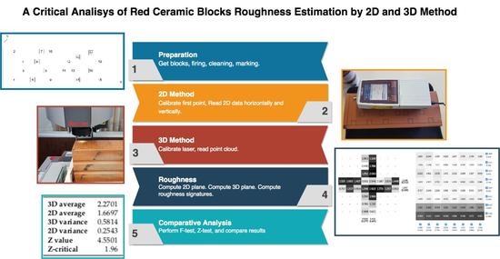
This work quantifies and compares the roughness obtained with the use of two measuring equipment, a rugosimeter, and a 3D laser profilometer, verifying the variations in results between the two measuring methods and formulating a critical analysis regarding the quality of the information obtained with each equipment. Red ceramic blocks with different roughness were used to guarantee the control variable of this research.
2. Materials and Methods
In order to perform the roughness measurements, raw red ceramic blocks with dimensions of 9 cm × 14 cm × 24 cm were collected in a red ceramic plant located in the Vale dos Sinos region/RS, Brazil. In the laboratory, the raw blocks were separated into four groups and fired at firing temperatures of C, C, C, and C, with the objective of providing four groups of blocks with different surface topographies. The same clay was used with different firing cycles, with the consideration that clays coming from different compositions may generate alterations in the surface characteristics of the specimens that would be added to the changes resulting from the measurement type, generating an uncontrolled variable in the experimental program.
The raw blocks were dried in a kiln at
C for a period of 24 h. The firing cycle was done in a muffle furnace with a ramp of
C/hour until the desired temperature was reached, following the study of [
48]. The desired temperature (
C,
C,
C, or
C) were kept for 10 h, generating blocks with distinct characteristics, named samples type 7, 8, 9, and 10.
For materials with homogeneous roughness, such as metals, only one line was read to measure the roughness. However, for ceramic materials, where the surface roughness is heterogeneous, one line is not representative. For this reason, in this work 2 vertical and 2 horizontal were read to obtain a better representation. In the 3D method, all points on the surface were considered. In this way, roughness measurements were made on 4608 regions (gray cells of the roughness signature); resulting in 1536 values using 2D and 3072 values using 3D methods. Two data acquisition equipment were used, a two-dimensional contact-type rugosimeter Mitutoyo SJ-210/178-561-02A, with a stylus tip radius of 5 μm, with tip angle 90 and detector measuring force of 4 nM; and a three-dimensional laser profilometer Starrett AV300+, with X-Y Accuracy (μm): , Z Accuracy (μm): , and scale resolution 0.1 μm.
The average roughness parameters (
), which is the arithmetic average of all the peaks and valleys of the evaluated profile, were determined for the data obtained in the two acquisition methods. The parameter used, average roughness
, described in [
27,
40], is given by:
Figure 3, presented in [
27,
40], illustrates the behavior of the parameter in relation to a profile of a sampled surface.
After determining the roughness parameters for each area, the results were analyzed using the average and standard deviation of the parameter in order to compare the data found in the 2D and 3D methods, verified if they vary significantly from one another.
The roughness was evaluated on four squared surfaces with 10 mm on each side surface of the blocks, selected of the 19 positions indicated in
Figure 4, according to the need to evaluate the variability of the surface of each block. In all blocks the markings are in the same position. The process of choosing areas took place qualitatively with a single observer, avoiding squares with deformations, so it was necessary to analyze all surfaces before choosing each 1 cm
area. The markings were made according to the availability of areas without macro-scale imperfections on the faces of the blocks. In each block, 4 out of 19 possible locations were selected, excluding those with imperfections.
Figure 4 presents the general process defined for the study.
The two-dimensional quantitative analyses with contact were performed following the procedure recommended by NBR ISO 4287 [
49],which specifies the method for measuring
2D using in-line measurement in one direction, to compose the roughness determination profile. The samples were previously cleaned with a compressed air jet and dried in a kiln at
C. In each block, linear surface profiles were measured in areas of 10 mm × 10 mm (
Figure 4). The data acquisition process is illustrated in
Figure 5.
The scanning of the profile is performed from the needle contact, without change to the roughness of the material. The measurements occurred in the horizontal and vertical direction, in order to verify if when changing the analysis orientation the roughness presents a significantly similar or distinct behavior. Parameter
was calculated.
Figure 6 presents the process for computing roughness for 2D data. The same mathematical equation used for the data acquisition equipment was used in the calculation of
.
As there is no agreed method for the determination of the roughness of ceramic blocks, the study proposes to determine whether the use of the 2D method specified by NBR ISO 4287 [
49] is suitable for the determination of the roughness of red ceramic substrates. For the formulation of the experimental program, it was assumed that the heterogeneity of red ceramic substrates is high and much higher than that found on metal surfaces, where the determination of roughness by two-dimensional (in-line) methods is a consolidated practice. If the hypothesis is validated, the method is not considered suitable for the determination of
on ceramic substrates. After data acquisition with 2D equipment, it was verified whether the change in sampling direction results in a significant difference in
. To perform this statistical analysis, the hypothesis test from the variances is used to check whether there is sufficient evidence, at the
significance level, that the variances of
measured in the horizontal direction are equal to the variances of
measured in the vertical direction (corresponding to the
x and
y axes represented in
Figure 4). A second analysis checked whether the
determined from data collection in only one line is representative for defining the
of the substrate. For this purpose, it was ascertained whether there is sufficient evidence, at the
significance level, to confirm the similarity in determining
between single-line groups measured in the same sampling direction.
In addition to 2D analysis, quantitative, three-dimensional, and non-contact roughness analysis was performed using the laser profilometer 3D, named 3D analysis. Before measurements, each surface was cleaned with a compressed air jet and dried in a kiln at
C. From the markings made on the blocks (as shown in
Figure 4), a total of 48 samples qualitatively selected with areas of 100 mm
with a pitch of 10 μm were analyzed, totaling the acquisition of data clouds with about 10,000 points in each sample, from which the roughness values (
) were calculated. The equipment works with the movement of a head over the parts making the measurements of the
x and
y-axis, while simultaneously measuring the
z-axis with the laser. After processing the data, it was transferred to the equipment’s software and converted into a three-dimensional point cloud.
To obtain results of the roughness parameters on the 3D point cloud, the method proposed by [
40] was used. For each point cloud an fitting plane is computed, which describes the average surface of the cloud (as shown in
Figure 7). The fitting plane is calculated by the least squares method and the roughness parameters are distances on the
Z axis of each point from the plane. When the distance from the point to the plane is positive, the point is considered a peak, when the distance is negative, the point is considered a valley. Roughness is therefore an average of peak to valley distances from the point cloud.
In order to provide a greater level of detail for the surface roughness analysis, the surface is divided into regions of the same size within the various levels of representation. A quadtree was adopted that divides the surface in a hierarchical structure to represent the roughness data in levels of detail.
Figure 8 shows an example of roughness coefficients represented at different levels of the quadtree. In the 4th level of the quadtree, the sample area is divided into
nodes (parts or gray cells in roughness signature) of the surface, allowing individual analysis in 64 regions of each sampled surface, as seen in
Figure 9. For each node, the roughness parameters are computed and statistical data are calculated for comparative analysis. Only one fitting plane is computed for the surface point cloud. Therefore, the average roughness (
) of each node (at all levels of the quadtree) is the average of the distances between each point in the region (node) and the surface plane.
The method also proposes a graphical representation of the roughness parameters along the surface, called the roughness signature. A quantitative analysis was possible and with a better level of detail through the statistical data computed for each surface node. In the results presented by the method it was possible to identify regions with more or less roughness along the surface generated by the same cloud of data.
Figure 9 presents the result obtained from the method proposed in [
40] with a sample among the 100 mm
areas obtained in this study. In the roughness signature (the gray cells), it can be noted that the roughness is not homogeneous along the surface (there are differences among the
values determined for each of the 64 regions into which the 100 mm
surface area has been divided). The roughness assessment method proposed in [
40] allows to observe the roughness behavior over the entire surface area. In the line chart and in the darker cells of the lines below the roughness signature (
Figure 9), a different behavior related to the roughness values is perceived. Probably, these noise are generated during the manufacturing process, by the handling or by the firing of the ceramic blocks. The histogram shows the distribution of
values between the minimum
and the maximum
, indicating where the highest concentration of
is in the sample.
Since the 3D method analyzes points without a specific direction, direct statistical comparison between the 2D and 3D methods is not appropriate. Thus, it is necessary to adjust the data acquired by the 2D rugosimeter in order to consider the analysis of a point cloud containing data in both horizontal and vertical directions, that is, independent of direction. The method proposed in this study consists of calculating the adjustment plane for the values obtained between 2D lines on the same surface, and from this plane the calculation of
, using the method described above for 3D analysis. The adjustment plane was calculated for all the data acquired from the same sample in 2D. For this purpose, the data concerning the height of the point in the 2D method is defined as the
Z-coordinate and the data concerning the position of the horizontal lines is defined as the
X-coordinate. Any value between 0 to 1 was defined as the
Y-coordinate. In the specific case, for the first row a value of
has been assigned and for the second row a value of
has been assigned in such a way that the data are close to the sampled region and do not collide with each other. The same is true for data on vertical lines, but the position coordinate for the
Y- and
X-coordinate were
and
, assigned respectively for the first line and second line. After redefining the point cloud from 2D to 3D and calculating the adjustment plane, the hierarchical subdivision of regions (quadtree) was carried out and the
was calculated for each node as defined by [
40]. The mean roughness (
) and standard deviation (
) data of each sample were also calculated, at the same level of detail as the proposed tree in [
40], the third level.
Figure 10 shows the result of the roughness signature for a 2D sample, obtained from the acquisition of two horizontal and two vertical lines by the 2D method and subsequent data adjustment. The nodes (regions) in the sample which do not have associated values are those corresponding to regions where 2D sampling was not performed. It is important to note that each rectangular line, vertical or horizontal, represents a 2D sampled line and that each node contains 250 points, with the exception of the nodes which coincide with the two directions, which have 500 points. Those regions that do not have values (which are filled with dashes) are those which do not coincide with any sampled value.
From the definition of the calculation procedure, it was possible to compare the results of 2D and 3D sampling. The objective is to determine if there is a significant difference between the roughness determination with the 2D method and the 3D method, evaluating if there is an advantage in using the 3D method over the 2D method. Validation has been carried out by means of hypothesis testing (Z-test), at the
significance level, to confirm that the means of
using the 3D method are similar to the means of
using the 2D method. The Z-test is used, since 48 samples are analyzed, with normal distribution, instead of the T-test (appropriate for sample sizes below 30).
Section 3 will present the comparative data between the two methods for measuring roughness, as well as the statistical analyses and considerations on the results.
3. Results
In order to compare the two methods of measuring roughness, statistical analyses were carried out and are presented under this topic.
The first analysis assessed whether there is a significant difference in the direction of measurement by the 2D method. The F-test of hypotheses from the standard deviations was used. The mean
values per sample, obtained by capturing data in one row (two-dimensional data), are presented in
Table 1, and
Table 2 presents the results of the comparison of the differences in roughness between two data captures in parallel rows and between data captures in perpendicular rows to each other.
When comparing the vertical and horizontal lines obtained from the 2D analysis, performed on 10 mm × 10 mm fields of the same block, there is sufficient evidence, at the significance level, to confirm that the standard deviation variances of in horizontal and vertical directions are different from each other, depending on the sampling positions.
When comparing two measures of parallel roughness with each other, there is also sufficient evidence, at the significance level, to confirm that the standard deviation variances of for groups of two lines in the same sampling direction are different from each other, depending on the sampling position.
To determine if there is a significant difference between the estimation of
on ceramic block surfaces by the 2D roughness determination method and that obtained by the 3D method, the methodology described in
Section 2 has been used, performing the calculation of the fitting plane of the
data for the 2D samples. The aim is to determine whether there is an advantage in using the 3D method over the 2D method. For this purpose, a hypothesis test (Z test) at a
significance level was performed to confirm that the means of
using the 3D method are similar to the means using the 2D method.
Table 3 shows the data used in 3D and adjusted 2D for the test.
Table 4 shows the result of the Z-test performed from the data of
Table 3.
As shown in
Table 4, the result of the Z-test for similarity checking resulted in
F = 4.5501 and
F-critico = 1.96, which indicates that there is a significant difference between the two methods for determining the roughness of ceramic blocks.
In addition to this determination, carried out on the basis of group variances, a comparison was also made between the means in order to quantitatively verify the differences of in the population sampled from the two methods of analysis.
In the red ceramic substrates studied, a significantly higher
was observed using the 3D method when compared to the 2D method (the mean
found in the 2D sample is
of the mean value found by the 3D method, according to the data observed in
Table 3). To show this behavior, the
values are organized into ranges with uniform intervals.
Table 5 is assembled based on the histogram of
values, from both 2D and 3D data.
Table 6 and
Figure 11 shows the result of grouping
by method and by
value range. Note the significant difference in distribution ranges, where in the 2D method the highest concentration of values is in the initial ranges (lowest
values) and in the 3D method, the values are better distributed in all ranges, corroborating with the statement that the
in the 3D method is significantly higher.
4. Discussion
Regarding the sample acquisition methodology performed in this work, it was possible to establish standardization, repeatability, and maintain exemption to variables that cause failures in the data reading process and, consequently, in the results obtained. As was done in this work, it is recommended to use a template to standardize sample positions and care with block production as defined.
The difference between sampling directions (vertical and horizontal) using the 2D method, leads to believe that grooves are generated in the forming stage of the ceramic block as a function of the contact between the ceramic mass and the walls of the mold of the extruder during the extrusion process, in accordance with Sahoo [
21].
It is also noted that a difference in relation to the measurement position of the samples in the same direction, in lines parallel to each other, is obtained by the 2D method. It is estimated that this anisotropy is a function of the high variability in the composition of the clays used in the manufacture of red ceramic blocks, generating changes in roughness on a micrometric scale, and not only due to imperfections generated in the extrusion process of the block.
It can be seen that the 2D measurement site on red ceramic substrates changes the roughness parameters because depending on the sampling position there are significant differences in
, either between lines in the same direction or in different directions. It is concluded that the roughness of a ceramic block must not be determined from the 2D measurement at a single location, agreeing with the assumptions of [
41,
42,
43].
Regarding the difference between the two methods of determining the roughness of ceramic blocks, it concludes that the determination of the surface roughness of ceramic substrates by the 2D and 3D methods results in significantly different results.
In the studied red ceramic substrates, a significantly higher
was observed using the 3D method when compared to 2D. The difference in
as a function of the measurement method was also observed by Cristea et al. [
39] on other types of substrate.
In view of the differences between the methods for determining roughness, it is estimated that the method which best represents the roughness of the ceramic block surfaces is the 3D method, as proposed by [
12,
26].
Besides the heterogeneity of the red ceramic substrate, a second reason for the difference in roughness between the two methods is the measurement resolution of the 3D equipment (which makes the data acquisition by a laser beam), while the data acquisition needle size of the 2D equipment (4 μm) can generate smaller
values, as it cannot enter peaks and valleys that have a high amplitude and high frequency configuration (seen in
Figure 2), while the laser used in the 3D method can read these peaks and valleys with a higher reading resolution, generating higher roughness parameters than those obtained in the 2D method. It is estimated that the smallest standard deviation observed in 2D analysis occurs because with the contact method only one surface profile was captured and several valleys were attenuated according to the needle dimensions, while in the three-dimensional method, besides capturing valleys with greater amplitude and frequency, an area of
mm × 10 mm was analyzed, which allowed the capture of a greater amount of surface roughness variations.


 ,
, 


