
Using Digital Photography to Track Understory Phenology in Mediterranean Cork Oak Woodlands

 ,
,  ,
,
Abstract
:
1. Introduction
2. Materials and Methods
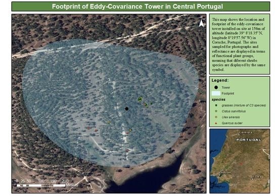
2.1. Site
2.2. Data
2.2.1. Climatic Variables
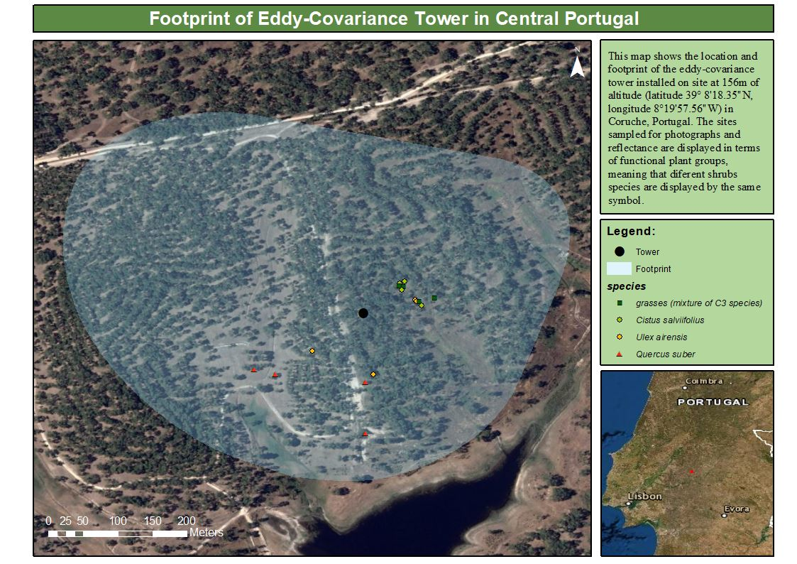
2.2.2. Digital Photographs and Reflectance Data
2.3. Vegetation Indices
2.3.1. Picture-Based Indices
2.3.2. Reflectance-Based Indices
2.4. Data Analysis
2.4.1. Vegetation Indices
2.4.2. Climate Variables
3. Results
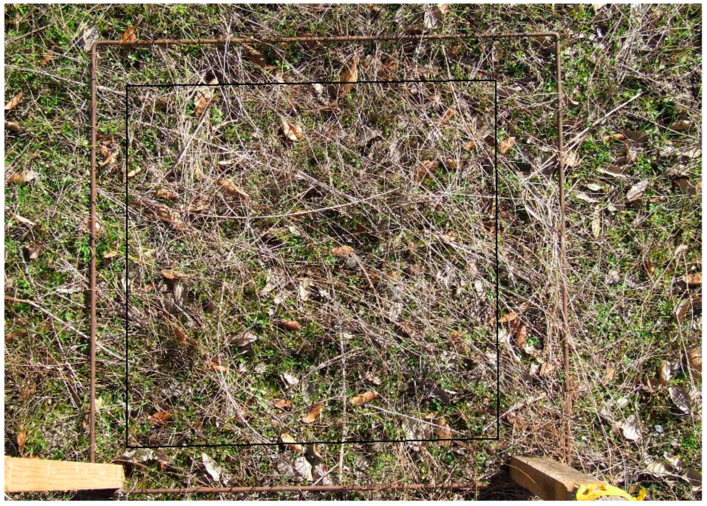
3.1. Climate
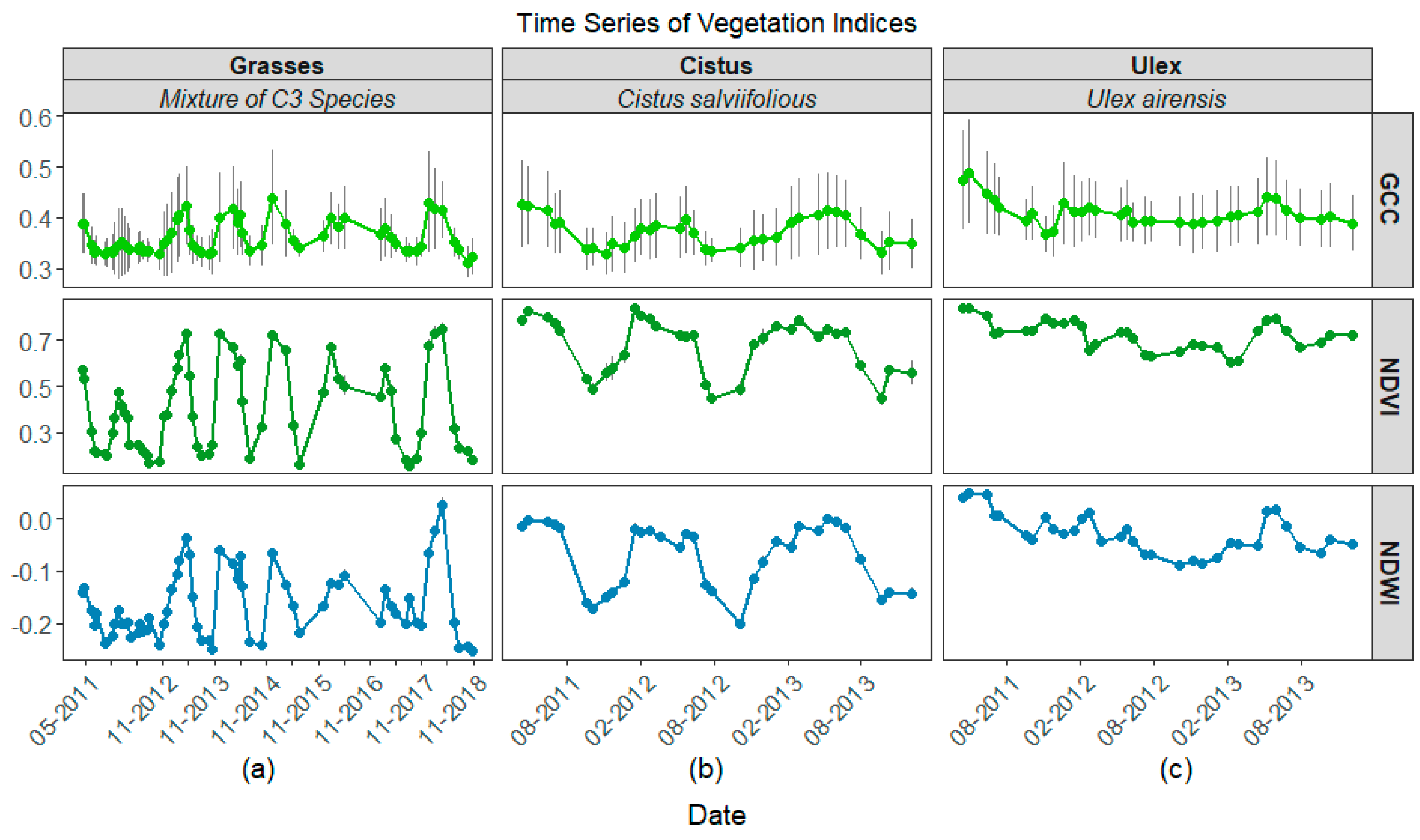
3.2. Time Series
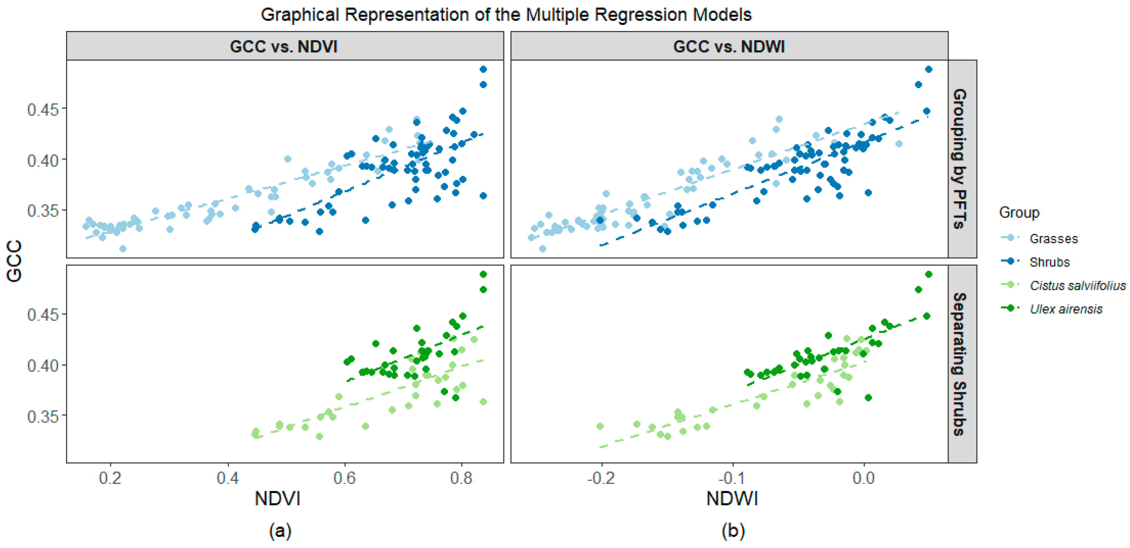
3.3. Association among Indices
3.4. Association between GCC and Climate Variables
4. Discussion
4.1. The Applicability of GCC
4.1.1. Time Series Analysis
4.1.2. Method Usefulness
4.2. Differences among Grasses, Cistus, and Ulex
4.3. Responsiveness of GCC to Climate
5. Conclusions
Supplementary Materials
Author Contributions
Funding
Institutional Review Board Statement
Informed Consent Statement
Data Availability Statement
Acknowledgments
Conflicts of Interest
References
- Menzel, A. Phenology: Its Importance to the Global Change Community. Clim. Chang. 2002, 54, 379–385. [Google Scholar] [CrossRef]
- Richardson, A.D.; Jenkins, J.P.; Braswell, B.H.; Hollinger, D.Y.; Ollinger, S.V.; Smith, M.-L. Use of digital webcam images to track spring green-up in a deciduous broadleaf forest. Oecologia 2007, 152, 323–334. [Google Scholar] [CrossRef]
- Crick, H.Q.P.; Dudley, C.; Glue, D.E.; Thomson, D.L. UK Birds Are Laying Eggs Earlier CO 2 Increases Oceanic Primary Production UK Birds Are Laying Eggs Earlier. Nature 1997, 388, 526. [Google Scholar] [CrossRef]
- Kramer, K.; Leinonen, I.; Loustau, D. The importance of phenology for the evaluation of impact of climate change on growth of boreal, temperate and Mediterranean forests ecosystems: An overview. Int. J. Biometeorol. 2000, 44, 67–75. [Google Scholar] [CrossRef]
- Luo, Y.; El-Madany, T.S.; Filippa, G.; Ma, X.; Ahrens, B.; Carrara, A.; Gonzalez-Cascon, R.; Cremonese, E.; Galvagno, M.; Hammer, T.W.; et al. Using Near-Infrared-Enabled Digital Repeat Photography to Track Structural and Physiological Phenology in Mediterranean Tree–Grass Ecosystems. Remote Sens. 2018, 10, 1293. [Google Scholar] [CrossRef] [Green Version]
- Bradley, B.A.; Jacob, R.W.; Hermance, J.F.; Mustard, J.F. A curve fitting procedure to derive inter-annual phenologies from time series of noisy satellite NDVI data. Remote Sens. Environ. 2007, 106, 137–145. [Google Scholar] [CrossRef]
- Porcar-Castell, A.; Mac Arthur, A.; Rossini, M.; Eklundh, L.; Pacheco-Labrador, J.; Anderson, K.; Balzarolo, M.; Martín, M.P.; Jin, H.; Tomelleri, E.; et al. EUROSPEC: At the interface between remote-sensing and ecosystem CO2 flux measurements in Europe. Biogeosciences 2015, 12, 6103–6124. [Google Scholar] [CrossRef] [Green Version]
- Soudani, K.; Hmimina, G.; Delpierre, N.; Pontailler, J.-Y.; Aubinet, M.; Bonal, D.; Caquet, B.; De Grandcourt, A.; Burban, B.; Flechard, C.; et al. Ground-based Network of NDVI measurements for tracking temporal dynamics of canopy structure and vegetation phenology in different biomes. Remote Sens. Environ. 2012, 123, 234–245. [Google Scholar] [CrossRef]
- Häusler, M.; Silva, J.M.N.; Cerasoli, S.; López-Saldaña, G.; Pereira, J.M.C. Modelling spectral reflectance of open cork oak woodland: A simulation analysis of the effects of vegetation structure and background. Int. J. Remote. Sens. 2016, 37, 492–515. [Google Scholar] [CrossRef]
- Migliavacca, M.; Galvagno, M.; Cremonese, E.; Rossini, M.; Meroni, M.; Sonnentag, O.; Cogliati, S.; Manca, G.; Diotri, F.; Busetto, L.; et al. Using digital repeat photography and eddy covariance data to model grassland phenology and photosynthetic CO2 uptake. Agric. For. Meteorol. 2011, 151, 1325–1337. [Google Scholar] [CrossRef]
- Keenan, T.F.; Darby, B.; Felts, E.; Sonnentag, O.; Friedl, M.A.; Hufkens, K.; O’Keefe, J.; Klosterman, S.; Munger, J.W.; Toomey, M.; et al. Tracking forest phenology and seasonal physiology using digital repeat photography: A critical assessment. Ecol. Appl. 2014, 24, 1478–1489. [Google Scholar] [CrossRef] [Green Version]
- Reid, A.M.; Chapman, W.K.; Prescott, C.E.; Nijland, W. Using excess greenness and green chromatic coordinate colour indices from aerial images to assess lodgepole pine vigour, mortality and disease occurrence. For. Ecol. Manag. 2016, 374, 146–153. [Google Scholar] [CrossRef]
- Sonnentag, O.; Detto, M.; Vargas, R.; Ryu, Y.; Runkle, B.; Kelly, M.; Baldocchi, D. Tracking the structural and functional development of a perennial pepperweed (Lepidium latifolium L.) infestation using a multi-year archive of webcam imagery and eddy covariance measurements. Agric. For. Meteorol. 2011, 151, 916–926. [Google Scholar] [CrossRef]
- Klosterman, S.T.; Hufkens, K.; Gray, J.M.; Melaas, E.; Sonnentag, O.; LaVine, I.; Mitchell, L.; Norman, R.; Friedl, M.A.; Richardson, A.D. Evaluating remote sensing of deciduous forest phenology at multiple spatial scales using PhenoCam imagery. Biogeosciences 2014, 11, 4305–4320. [Google Scholar] [CrossRef] [Green Version]
- Tang, J.; Körner, C.; Muraoka, H.; Piao, S.; Shen, M.; Thackeray, S.J.; Yang, X. Emerging opportunities and challenges in phenology: A review. Ecosphere 2016, 7, e01436. [Google Scholar] [CrossRef] [Green Version]
- Jarraud, M.; Steiner, A. Summary for Policymakers. Managing the Risks of Extreme Events and Disasters to Advance Climate Change Adaptation: Special Report. In Proceedings of the Intergovernmental Panel on Climate Change, Geneva, Switzerland, 6–9 June 2012; pp. 3–22. [Google Scholar] [CrossRef]
- Peñuelas, J.; Filella, I.; Comas, P.E. Changed Plant and Animal Life Cycles from 1952 to 2000 in the Mediterranean Region. Glob. Chang. Biol. 2002, 8, 531–544. [Google Scholar] [CrossRef] [Green Version]
- Gordo, O.; Sanz, J.J. Long-term temporal changes of plant phenology in the Western Mediterranean. Glob. Chang. Biol. 2009, 15, 1930–1948. [Google Scholar] [CrossRef]
- Schroeter, D.; Cramer, W.; Leemans, R.; Prentice, I.C.; Araújo, M.B.; Arnell, N.W.; Bondeau, A.; Bugmann, H.; Carter, T.R.; Gracia, C.A.; et al. Ecosystem Service Supply and Vulnerability to Global Change in Europe. Science 2005, 310, 1333–1337. [Google Scholar] [CrossRef] [PubMed] [Green Version]
- Chmielewski, F.-M.; Rötzer, T. Response of tree phenology to climate change across Europe. Agric. For. Meteorol. 2001, 108, 101–112. [Google Scholar] [CrossRef]
- Giorgi, F.; Lionello, P. Climate change projections for the Mediterranean region. Glob. Planet. Chang. 2008, 63, 90–104. [Google Scholar] [CrossRef]
- Piayda, A.; Dubbert, M.; Rebmann, C.; Kolle, O.; Costa e Silva, F.; Correia, A.; Pereira, J.S.; Werner, C.; Cuntz, M. Drought impact on carbon and water cycling in a Mediterranean Quercus suber L. woodland during the extreme drought event in 2012. Biogeosciences 2014, 11, 7159–7178. [Google Scholar] [CrossRef] [Green Version]
- Lecomte, X.J.F. Effects of Grazing Exclusion and Shrub Encroachment on the Ecosystem Ecology of Evergreen Oak Woodland, Instituto Superior de Agronomia, Universidade de Lisboa. 2018. Available online: http://hdl.handle.net/10400.5/15334 (accessed on 18 February 2021).
- Bugalho, M.N.; Caldeira, M.C.; Pereira, J.S.; Aronson, J.; Pausas, J.G. Mediterranean cork oak savannas require human use to sustain biodiversity and ecosystem services. Front. Ecol. Environ. 2011, 9, 278–286. [Google Scholar] [CrossRef] [Green Version]
- Dubbert, M.; Mosena, A.; Piayda, A.; Cuntz, M.; Correia, A.C.; Pereira, J.S.; Werner, C. Influence of tree cover on herbaceous layer development and carbon and water fluxes in a Portuguese cork-oak woodland. Acta Oecolog. 2014, 59, 35–45. [Google Scholar] [CrossRef]
- Correia, A.; Costa e Silva, F.C.; Correia, A.; Hussain, M.; Rodrigues, A.; David, J.; Pereira, J. Carbon sink strength of a Mediterranean cork oak understorey: How do semi-deciduous and evergreen shrubs face summer drought? J. Veg. Sci. 2013, 25, 411–426. [Google Scholar] [CrossRef]
- Richardson, A.D.; Keenan, T.F.; Migliavacca, M.; Ryu, Y.; Sonnentag, O.; Toomey, M. Climate change, phenology, and phenological control of vegetation feedbacks to the climate system. Agric. For. Meteorol. 2013, 169, 156–173. [Google Scholar] [CrossRef]
- Jongen, M.; Unger, S.; Fangueiro, D.; Cerasoli, S.; Silva, J.M.; Pereira, J.S. Resilience of montado understorey to experimental precipitation variability fails under severe natural drought. Agric. Ecosyst. Environ. 2013, 178, 18–30. [Google Scholar] [CrossRef] [Green Version]
- Molina, J.R.; Prades, C.; Lora, Á.; Silva, F.R.Y. Quercus suber cork as a keystone trait for fire response: A flammability analysis using bench and field scales. For. Ecol. Manag. 2018, 429, 384–393. [Google Scholar] [CrossRef]
- Jongen, M.; LeComte, X.; Unger, S.; Pinto-Marijuan, M.; Pereira, J.S. The impact of changes in the timing of precipitation on the herbaceous understorey of Mediterranean evergreen oak woodlands. Agric. For. Meteorol. 2013, 171, 163–173. [Google Scholar] [CrossRef]
- Unger, S.; Máguas, C.; Pereira, J.S.; Aires, L.M.I.; David, T.S.; Werner, C. Partitioning carbon fluxes in a Mediterranean oak forest to disentangle changes in ecosystem sink strength during drought. Agric. For. Meteorol. 2009, 149, 949–961. [Google Scholar] [CrossRef]
- Instituto Português do Mar e da Atmosfera (IPMA). Normais Climatológicas 1971–2000. 2019. Available online: https://www.ipma.pt/pt/oclima/normais.clima/1971-2000/ (accessed on 24 September 2019).
- Cerasoli, S.; Costa e Silva, F.; Portugal, J.; Moura, C.F.; Carvalhais, N.; Pereira, J.S.; David, J.S.; Migliavacca, M.; El-Madany, T. Carbon and Water Fluxes in a Cork Oak Woodland in Central Portugal. Zenodo 2020, 1, 3727798. [Google Scholar] [CrossRef]
- Cerasoli, S.; Costa e Silva, F.; Silva, J.M.N. Temporal dynamics of spectral bioindicators evidence biological and ecological differences among functional types in a cork oak open woodland. Int. J. Biometeorol. 2015, 60, 813–825. [Google Scholar] [CrossRef]
- Malthus, T.J.; MacLellan, C.J. High Performance Fore Optic Accessories and Tools for Reflectance and Radiometric Measurements with the ASD FieldSpec 3 Spectroradiometer. In Proceedings of the Art, Science and Applications of Reflectance Spectroscopy, Boulder, CO, USA, 23–25 February 2010; pp. 1–5. [Google Scholar]
- Lewis, G.V.; Catlow, C.R.A. Potential models for ionic oxides. J. Phys. C Solid State Phys. 1985, 18, 1149–1161. [Google Scholar] [CrossRef]
- Richardson, A.D.; Braswell, B.H.; Hollinger, D.Y.; Jenkins, J.P.; Ollinger, S.V. Near-surface remote sensing of spatial and temporal variation in canopy phenology. Ecol. Appl. 2009, 19, 1417–1428. [Google Scholar] [CrossRef]
- Filippa, G.; Cremonese, E.; Migliavacca, M.; Galvagno, M.; Forkel, M.; Wingate, L.; Tomelleri, E.; Di Cella, U.M.; Richardson, A.D. Phenopix: A R package for image-based vegetation phenology. Agric. For. Meteorol. 2016, 220, 141–150. [Google Scholar] [CrossRef] [Green Version]
- Rouse, J.W.; Hass, R.H.; Schell, J.A.; Deering, D.W. Monitoring Vegetation Systems in the Great Plains with ERTS. In Proceedings of the Third Earth Resources Technology Satellite-1 (ERTS) Symposium: The Proceedings of a Symposium Held by Goddard Space Flight Center, Washington, DC, USA, 10–14 December 1973; Volume 1, pp. 309–317.
- Gao, B.-C. NDWI—A normalized difference water index for remote sensing of vegetation liquid water from space. Remote Sens. Environ. 1996, 58, 257–266. [Google Scholar] [CrossRef]
- Brian, A.; Peterson, G.; Carl, P.; Boudt, K.; Bennett, R.; Ulrich, J.; Zivot, E.; Lestel, M.; Balkissoon, K. Package “PerformanceAnalytics”. Econom. Tools Perform. Risk Anal. 2018, 2, 240. [Google Scholar]
- Marchin, R.M.; McHugh, I.; Simpson, R.R.; Ingram, L.J.; Balas, D.S.; Evans, B.J.; Adams, M.A. Productivity of an Australian mountain grassland is limited by temperature and dryness despite long growing seasons. Agric. For. Meteorol. 2018, 116–124. [Google Scholar] [CrossRef]
- Pettorelli, N. NDVI and Environmental Monitoring; NDVI and Plant Ecology. In Normalized Difference Vegetation Index; Oxford University Press: Oxford, UK, 2013; Chapters 5–6; pp. 56–80. [Google Scholar]
- Wingate, L.; Ogee, J.; Cremonese, E.; Filippa, G.; Mizunuma, T.; Migliavacca, M.; Moisy, C.; Wilkinson, M.; Moureaux, C.; Wohlfahrt, G.; et al. Interpreting canopy development and physiology using a European phenology camera network at flux sites. Biogeosciences 2015, 12, 5995–6015. [Google Scholar] [CrossRef] [Green Version]
- Cremonese, E.; Filippa, G.; Galvagno, M.; Siniscalco, C.; Oddi, L.; Di Cella, U.M.; Migliavacca, M. Heat wave hinders green wave: The impact of climate extreme on the phenology of a mountain grassland. Agric. For. Meteorol. 2017, 247, 320–330. [Google Scholar] [CrossRef]
- Jongen, M.; Pereira, J.S.; Aires, L.M.I.; Pio, C.A. The effects of drought and timing of precipitation on the inter-annual variation in ecosystem-atmosphere exchange in a Mediterranean grassland. Agric. For. Meteorol. 2011, 151, 595–606. [Google Scholar] [CrossRef]
- Bolton, D.K.; Friedl, M.A. Forecasting crop yield using remotely sensed vegetation indices and crop phenology metrics. Agric. For. Meteorol. 2013, 173, 74–84. [Google Scholar] [CrossRef]
- Gu, Y.; Brown, J.F.; Verdin, J.P.; Wardlow, B. A five-year analysis of MODIS NDVI and NDWI for grassland drought assessment over the central Great Plains of the United States. Geophys. Res. Lett. 2007, 34, 1–6. [Google Scholar] [CrossRef] [Green Version]
- Correia, A.; Costa-E-Silva, F.; Dubbert, M.; Piayda, A.; Pereira, J. Severe dry winter affects plant phenology and carbon balance of a cork oak woodland understorey. Acta Oecologica 2016, 76, 1–12. [Google Scholar] [CrossRef]
- Cerasoli, S.; Campagnolo, M.; Faria, J.; Nogueira, C.; Caldeira, M.D.C. On estimating the gross primary productivity of Mediterranean grasslands under different fertilization regimes using vegetation indices and hyperspectral reflectance. Biogeosciences 2018, 15, 5455–5471. [Google Scholar] [CrossRef] [Green Version]
- Rautiainen, M.; Mõttus, M.; Heiskanen, J.; Akujärvi, A.; Majasalmi, T.; Stenberg, P. Seasonal reflectance dynamics of common understory types in a northern European boreal forest. Remote Sens. Environ. 2011, 115, 3020–3028. [Google Scholar] [CrossRef]
- Migliavacca, M.; Cremonese, E.; Colombo, R.; Busetto, L.; Galvagno, M.; Ganis, L.; Meroni, M.; Pari, E.; Rossini, M.; Siniscalco, C.; et al. European larch phenology in the Alps: Can we grasp the role of ecological factors by combining field observations and inverse modelling? Int. J. Biometeorol. 2008, 52, 587–605. [Google Scholar] [CrossRef]
- Sonnentag, O.; Hufkens, K.; Teshera-Sterne, C.; Young, A.M.; Friedl, M.A.; Braswell, B.H.; Milliman, T.; O’Keefe, J.; Richardson, A.D. Digital repeat photography for phenological research in forest ecosystems. Agric. For. Meteorol. 2012, 152, 159–177. [Google Scholar] [CrossRef]
- Harley, P.C.; Tenhunen, J.D.; Beyschlag, W.; Lange, O.L. Seasonal changes in net photosynthesis rates and photosynthetic capacity in leaves of Cistus salvifolius, a European mediterranean semi-deciduous shrub. Oecologia 1987, 74, 380–388. [Google Scholar] [CrossRef]


| Vegetation Index | Formula | |
|---|---|---|
| Normalized Difference Vegetation Index | (2) | |
| Normalized Difference Water Index | (3) |
| Simple Linear Regressions | ||||
|---|---|---|---|---|
| NDVI | ||||
| Equation | r | r2 | p-value | |
| grasses | y = 16x1 + 0.30 | 0.945 | 0.89 | <0.05 |
| cistus | y = 0.20x1 + 0.24 | 0.793 | 0.62 | <0.05 |
| ulex | y = 0.24x1 + 0.24 | 0.564 | 0.30 | <0.05 |
| NDWI | ||||
| Equation | r | r2 | p-value | |
| grasses | y = 0.45x1 + 0.43 | 0.917 | 0.84 | <0.05 |
| cistus | y = 0.41x1 + 0.40 | 0.885 | 0.78 | <0.05 |
| ulex | y = 0.51x1 + 0.42 | 0.754 | 0.55 | <0.05 |
| Models Separating Vegetation by PFT | |||||
|---|---|---|---|---|---|
| NDVI | |||||
| Coefficients: | |||||
| Estimate | Std. Error | t value | Pr (>|t|) | Residual standard error: 0.01885 on 124 DF | |
| (Intercept) | 0.296693 | 0.005656 | 52.452 | < 2 × 10⁻¹⁶ *** | |
| NDVI | 0.161242 | 0.013046 | 12.360 | < 2 × 10⁻¹⁶ *** | Adjusted R-squared: 0.7274 |
| PFT | −0.073573 | 0.017942 | −4.101 | 7.4 × 10⁻⁵ *** | F-statistic: 113.9 |
| NDVI×PFT | 0.080054 | 0.027463 | 2.915 | 0.00422 ** | p-value = 0.05 |
| NDWI | |||||
| Coefficients: | |||||
| Estimate | Std. Error | t value | Pr (>|t|) | Residual standard error: 0.01562 on 124 DF | |
| (Intercept) | 0.434724 | 0.005529 | 78.628 | <2 × 10⁻¹⁶ *** | |
| NDWI | 0.445858 | 0.030808 | 14.472 | <2 × 10⁻¹⁶ *** | Adjusted R-squared: 0.8128 |
| PFT | −0.018052 | 0.006100 | −2.960 | 0.00369 ** | F-statistic: 184.8 |
| NDWI×PFT | 0.060766 | 0.046307 | 1.312 | 0.19186 | p-value: < 2.2 × 10⁻¹⁶ |
| Models with Shrub Distinction | |||||
|---|---|---|---|---|---|
| NDVI | |||||
| Coefficients: | |||||
| Estimate | Std. Error | t value | Pr (>|t|) | Residual standard error: 0.02009 on 62 DF | |
| (Intercept) | 0.2395414 | 0.0205342 | 11.665 | <2 × 10⁻¹⁶ *** | |
| NDVI | 0.1972340 | 0.0299884 | 6.577 | 1.15 × 10⁻⁸ *** | Adjusted R-squared: 0.6406 |
| PFT shrubs | 0.0007734 | 0.0461891 | 0.017 | 0.987 | F-statistic: 39.62 |
| NDVI×PFT shrubs | 0.0386738 | 0.0645447 | 0.599 | 0.551 | p-value: 2.01× 10⁻¹⁴ |
| NDWI | |||||
| Coefficients: | |||||
| Estimate | Std. Error | t value | Pr (>|t|) | Residual standard error: 0.01577 on 62 DF | |
| (Intercept) | 0.402185 | 0.004186 | 96.084 | < 2 × 10⁻¹⁶ *** | |
| NDWI | 0.414499 | 0.044312 | 9.354 | 1.84 × 10⁻¹³ *** | Adjusted R-squared: 0.7787 |
| PFT shrubs | 0.022588 | 0.005405 | 4.179 | 9.34 × 10⁻⁵ *** | F-statistic: 77.25 |
| NDWI×PFT shrubs | 0.098773 | 0.085586 | 1.154 | 0.253 | p-value: < 2.2 × 10⁻¹⁶ |
| Grasses | Selected Variable | t Value | Pr (>|t|) | |
| Tmax30 (r = −0.66) | −3.793 | 0.000383 *** | Adjusted R-squared: 0.5419 | |
| Prec90 (r = 0.66) | 3.813 | 0.000360 *** | p-value: 3.882 × 10⁻¹⁰ | |
| cistus | Selected Variable | |||
| Tmax90 (r = −0.63) | −3.393 | 0.00196 *** | Adjusted R-squared: 0.3786 | |
| Prec90 (r = 0.44) | 1.063 | 0.29611 | p-value: 0.0003021 | |
| ulex | Selected Variable | |||
| Tmin90 (r = −0.37) | −1.739 | 0.0924 | Adjusted R-squared: 0.1215 | |
| Prec90 (r = 0.31) | 1.177 | 0.2483 | p-value: 0.05441 |
Publisher’s Note: MDPI stays neutral with regard to jurisdictional claims in published maps and institutional affiliations. |
© 2021 by the authors. Licensee MDPI, Basel, Switzerland. This article is an open access article distributed under the terms and conditions of the Creative Commons Attribution (CC BY) license (http://creativecommons.org/licenses/by/4.0/).
Share and Cite
Jorge, C.; Silva, J.M.N.; Boavida-Portugal, J.; Soares, C.; Cerasoli, S. Using Digital Photography to Track Understory Phenology in Mediterranean Cork Oak Woodlands. Remote Sens. 2021, 13, 776. https://doi.org/10.3390/rs13040776
Jorge C, Silva JMN, Boavida-Portugal J, Soares C, Cerasoli S. Using Digital Photography to Track Understory Phenology in Mediterranean Cork Oak Woodlands. Remote Sensing. 2021; 13(4):776. https://doi.org/10.3390/rs13040776
Chicago/Turabian StyleJorge, Catarina, João M. N. Silva, Joana Boavida-Portugal, Cristina Soares, and Sofia Cerasoli. 2021. "Using Digital Photography to Track Understory Phenology in Mediterranean Cork Oak Woodlands" Remote Sensing 13, no. 4: 776. https://doi.org/10.3390/rs13040776