Technical Note

Annual Sea Level Amplitude Analysis over the North Pacific Ocean Coast by Ensemble Empirical Mode Decomposition Method

1
Department of Communications, Navigation and Control Engineering, National Taiwan Ocean University, Keelung 20224, Taiwan
2
Department of Geomatics, National Cheng Kung University, Tainan 70101, Taiwan
3
Department of System Engineering and Naval Architecture, National Taiwan Ocean University, Keelung 20224, Taiwan
*
Author to whom correspondence should be addressed.
Remote Sens. 2021, 13(4), 730; https://doi.org/10.3390/rs13040730
Submission received: 20 January 2021 / Revised: 11 February 2021 / Accepted: 12 February 2021 / Published: 17 February 2021
(This article belongs to the Special Issue Satellite Altimetry: Technology and Application in Geodesy)

Abstract

:
Understanding spatial and temporal changes of seasonal sea level cycles is important because of direct influence on coastal systems. The annual sea level cycle is substantially larger than semi-annual cycle in most parts of the ocean. Ensemble empirical mode decomposition (EEMD) method has been widely used to study tidal component, long-term sea level rise, and decadal sea level variation. In this work, EEMD is used to analyze the observed monthly sea level anomalies and detect annual cycle characteristics. Considering that the variations of the annual sea level variation in the Northeast Pacific Ocean are poorly studied, the trend and characteristics of annual sea level amplitudes and related mechanisms in the North Pacific Ocean are investigated using long-term tide gauge records covering 1950–2016. The average annual amplitude of coastal sea level exhibits interannual-to-decadal variability within the range of 14–220 mm. The largest value of ~174 mm is observed in the west coast of South China Sea. In the other coastal regions of North Pacific Ocean, the mean annual amplitude is relatively low between 77 and 124 mm for the western coast and 84 and 87 mm for the eastern coast. The estimated trend values for annual sea level amplitudes in the western coastal areas of South China Sea and Northeast Pacific Ocean have statistically decreased over 1952–2014 with a range of −0.77 mm·yr−1 to −0.11 mm·yr−1. Our results suggested that the decreasing annual amplitude in the west coast of South China Sea is in good agreement with the annual mean wind stress associated with the Pacific Decadal Oscillation (PDO). This wind phenomenon also explains the temporal variations of annual sea level amplitude in Northeast Pacific Ocean, especially the high correlations since 1980 (R = 0.61−0.72).

Graphical Abstract

1. Introduction

Seasonal cycle is a common signal in sea level change and fluctuates due to various physical forces, including atmospheric pressure, wind stress, precipitation, river runoff, ice melting, ocean current, and steric component [1]. Thus, the temporal sea level change in seasonality (annual and semi-annual) is not constant with time. Understanding seasonal sea level cycles and its spatial and temporal changes is important because its temporal changes (amplitude or phase) may directly affect the coastal systems [2]. An increase in the amplitude of seasonal sea level cycle during storm surge season also increases the risk of coastal flooding and coastal erosion. Thus, accurately estimating the seasonal amplitude and phase in sea level cycle and understanding the physical mechanisms of the seasonal sea level cycle are helpful in assessing the impact of future climate change on coastal ocean environments.
Early studies of seasonal sea level cycle are based on tide gauge records [3], which are limited in coastal areas. Since the early 1990s, satellite altimetry has provided near-global and high-quality observations of sea surface heights. Accuracy of satellite altimetric measurements is higher than 3 cm in open ocean, but rapidly decreases in marginal seas and when approaching coastal area [4,5]. This technique examines seasonal sea level cycle with high spatial coverage and resolution in coastal and open oceans. Chen et al. [6] used satellite altimetry and steric component to analyze seasonal sea level cycle on a global scale. Their results indicated that thermal effect has a dominant impact on observed seasonal variability, especially for zonal averages over regions. Vinogradov et al. [7] investigated seasonal sea level cycle in a near-global ocean by using satellite altimetry and an ocean circulation model. Their results indicated that annual cycle is substantially larger than semi-annual cycle in most parts of the ocean, except in tropical regions. They suggested that surface wind stress and heat flux are the main driving factors for seasonal sea level variations in tropical and mid-latitude regions, respectively, and these two mechanisms play a role at high-latitude regions. Vinogradov and Ponte [8] found that the spatial variability of annual sea level cycle varies from the shoreline to the adjacent shallow and deep ocean areas. The annual amplitude from tide gauge records is critically greater than that of nearby altimetry possibly due to the observations being conducted at different locations, inadequacy of some corrections, or a smoothing of the gridded altimetric data [9]. Wahl et al. [2] reported that the annual amplitude of sea level cycle has gradually increased along the United States Gulf coast since 1990s. They suggested that sea surface temperature and sea level pressure are the reason for the amplitude increase. Feng et al. [10] indicated that wind forcing and steric component are dominant impacts on the marginal seas and deep ocean (or open ocean) of the northwest Pacific Ocean, respectively. Amiruddin et al. [11] also reported similar results in the South China Sea. The temporal variation of seasonal sea level cycle has been investigated at regional scales, such as by Wahl et al. [2] for the United States Gulf coast, Feng et al. [10] and Amiruddin et al. [11] for the northwest Pacific coast, Torres and Tsimplis [12] for the Caribbean Sea, and Passaro et al. [13] and Cheng et al. [14] for the Baltic Sea and North Sea, respectively. Only a few studies have been conducted on seasonal sea level cycle in the Northeast Pacific Ocean. Hence, the driving factors behind temporal and spatial variations remain unrevealed.
The amplitude of seasonal sea level cycle exhibits decadal variability, such as in the Caribbean Sea [12], the United States Gulf coast [2], the South China Sea [11], and the northwest Pacific [10]. Related studies are based on traditional linear regression analysis (TLRA) method with 5-year overlapping periods (shifts month-by-month or year-by-year). This technique assumes that the amplitude and frequency of annual and semi-annual sea level cycles are constant within each time segment; hence, these parameters cannot reflect instantaneous changes and may be contaminated by other frequency signals when the window size is not appropriate [10]. The present study aims to detect changes in annual sea level cycle by using a developed ensemble empirical mode decomposition (EEMD) method [15] that could supplement the TLRA. Wu et al. [15] proposed a definition of a modulated annual cycle that allows the annual cycle to change from year to year by using a developed EEMD method [16]. This technique has been used for analyzing annual cycle in other geophysical data, such as surface air temperature and sea surface temperature [15,17].
Tide gauge stations are sparsely distributed in the early 20th century but rapidly increased in the 1950s [18]. In order to compute more accurate sea level trends and minimize the impact of low-frequency variability, all gauges needed at least 50 years of data [19,20]. EEMD is introduced to extract annual cycle data from observed sea level anomalies to analyze the trends and characteristics of annual sea level amplitude derived from long-term tide gauge records along the North Pacific Ocean coast covering 1950–2016. The dominant force is regionally identified to understand physical mechanisms responsible for sea level variability at the annual frequency. The rest of the paper is organized as follows. Data sets and methodology are described in Section 2 and Section 3, respectively. Results and discussion are reported in Section 4 and Section 5, and Section 6 offers conclusions.

2. Data Sets

2.1. Tide Gauge Records

Monthly mean sea level records at 316 tide gauge stations in the North Pacific Ocean were obtained from the Permanent Service for Mean Sea Level database [21,22]. Monthly records for Revised Local Reference were selected as the primary data set. If the data do not have substantial and unknown datum shifts, then some metric data were included [23]. All records provided at least 50 years of data between 1950 and 2016. The following tide gauge stations were excluded to avoid the influence of data gaps and large nonlinear signals due to typhoons, earthquakes, or groundwater pumping on the EEMD decomposition results [24]: those with data completeness of less than 90% within their time span, and those with records including nonlinear vertical land motion compared with neighboring tide gauge and altimeter measurements. Tide gauge data can be influenced by inverted barometer (IB) effect and contaminated by anomalous jumps owing to external forces and environmental changes [25]. In this study, IB effect and datum shift in tide gauge records were corrected according to tide gauge processing, introduced by Lan et al. [25]. In addition, individual tide gauge record with strong local effects was excluded to avoid the influence of local effect on the final outcome.
Monthly mean values of sea level time series from 107 tide gauge stations along North Pacific coast regions fulfilled the above criteria and are used in this study. Figure 1 shows the locations and record lengths of 107 tide gauge stations in the North Pacific Ocean. These tide gauges are classified into eight subregions (Table 1), namely the west coast of the South China Sea (SCSW), the East China Sea (ECS), the Sea of Japan (SJ), the northeast coasts of Japan (JNE), the southeast coasts of Japan (JSE), the Gulf of Alaska (GA), the west coast of Canada (WC), and the west coast of America (WA) (Figure 1).

2.2. Satellite Altimetric Data

Satellite altimetry has provided high-quality, global observations of sea surface height since early 1990s [4,5]. The altimeter data in this study are monthly gridded sea level anomaly maps at 0.25° × 0.25° spatial resolution with respect to a 20-year (1993–2012) mean sea level, which are provided by the Archiving, Validation, and Interpretation of Satellite Oceanographic (AVISO) data center (http://www.aviso.altimetry.fr/en/home.html, accessed on 19 January 2021), which are sea level anomaly products merged from several satellite altimetry missions of TOPEX/Poseidon, Jason-1/2, ERS-1/ERS-2, ENVISAT, GFO, Cryosat-2, Saral/AltiKa, and HY-2A. All standard corrections recommended by AVISO, including instrumental, medium (ionosphere, wet, and dry troposphere), and geophysical (solid earth, polar, ocean and load tides, sea state bias, and IB) corrections, were applied to the altimeter data. The data cover the period from January 1993 to December 2016. Altimetric observations at the closest grid points to the tide gauge location were compared with tide gauge data for the analysis of annual sea level cycle. The average distance between tide gauges and altimetric observations is approximately 10 km.

2.3. In Situ Hydrographical Data

Steric sea level variation was calculated from an updated version (v7.3) of in situ measurements of ocean temperature and salinity data processed by Ishii et al. [27] (called Ishii data hereinafter). This product has passed through several quality controls and provided monthly gridded fields with a spacing resolution of 1° × 1° and 28 vertical levels from the surface to 3000 m depth covering the period of 1955–2019. Steric sea level variation represents sea level change due to seawater density variation caused by fluctuations in ocean temperature and salinity. Its changes over water depth, hsteric, can be computed from seawater density change [28] expressed as:
h s t e r i c = z 1 z 2 ρ 0 ( S 0 , T 0 , z ) ρ ( S , T , z ) ρ 0 ( S 0 , T 0 , z ) d z ,
where S0 and T0 are the mean salinity and temperature, respectively; S and T are the monthly salinity and temperature of sea water, respectively; ρ and ρ0 are the density of water and the reference density of water, respectively; and z is the depth.

2.4. Wind Data

Surface wind stress was calculated using zonal and meridional (U and V) component winds obtained from the National Centers for Environmental Prediction (NCEP)/National Center for Atmospheric Research (NCAR) Reanalysis Monthly Means database (downloaded from https://www.psl.noaa.gov/, accessed on 19 January 2021) [29] by using bulk formulas [30]. This parameter provides monthly gridded fields from 1948 to present time with a spacing resolution of 2.5° × 2.5°. The IB effect was also removed from tide gauge records by using mean sea level pressure from NCEP/NCAR Reanalysis data set [29].

2.5. Climate Indices

Two natural modes of interannual/decadal variability, namely El Niño–Southern Oscillation (ENSO) and Pacific Decadal Oscillation (PDO), were analyzed to investigate the temporal variation of annual sea level amplitude in the North Pacific Ocean and the effect of low-frequency climate variability. These phenomena are typically considered the interannual and decadal variability with 2–8 and 10–30 years, respectively [31,32]. Their climate variabilities can be represented by the multivariate ENSO index (MEI) and PDO indices defined as the first unrotated principal component of six main observed variables (including sea-level pressure, zonal and meridional components of the surface wind, sea surface temperature, surface air temperature, and total cloudiness fraction of the sky) over the tropical Pacific (data source at: https://www.esrl.noaa.gov/psd/data/correlation/mei.data, accessed on 19 January 2021) and the leading principal component of North Pacific (poleward of 20° N in 1900–1993) monthly sea surface temperature anomalies (data source at: http://research.jisao.washington.edu/pdo/PDO.latest, accessed on 19 January 2021) [33,34], respectively. The two indices covered different time spans, that is, MEI for 1950 to 2016 and PDO for 1948 to 2016. For a clear description of the interannual and decadal characteristics of these two indicators, the MEI index was used to remove the MEI index with 65-month low-pass filter from low-passed MEI with 5-month filter, and the PDO index was smoothed with a 65-month running mean [35].

3. Methods

The analysis method is based on the Empirical Mode Decomposition (EMD), which is part of the Hilbert Huang Transform [36]. This method analyzes nonlinear and nonstationary time series, investigates the spatial and temporal characteristics of various data timescales [37,38], and it has been widely used to examine annual cycle in other geophysical data, such as surface air temperature and sea surface temperature [15,17]. The goal of EMD is to decompose a time series, x(t), into a set of components called intrinsic mode function (IMF), Ci(t), which can be expressed as:
X ( t ) = i = 1 n c i + r n ,
where n is the total number of IMFs, and n is close to but no more than log2 N, where N is the length of the input data, X(t) [39]. rn is the residual. Each IMF may represent different physical processes of various time scales from the highest frequency (IMF1) to the lowest frequency (IMFn), and the sum of all modes and residual can be used to reconstruct original data [40]. The decomposition process of EMD may produce mode mixing (one IMF component includes two or more different frequencies), so the ensemble EMD (EEMD) is applied for the considerable reduction of the mode mixing disparity [41], which can be expressed as:
X E ( t ) = X ( t ) + ε × n o i s e   ( t ) ,
where XE is the added noise data, X is original data, noise is the added white noise, andεis the amplitude of the added white noise. According to Wu and Huang [41], εis basically set to 0.2 standard deviation of the original data. However, when the data are dominated by high- or low-frequency signals, the noise amplitude may be small or large, respectively. These two steps were performed repeatedly by adding white noise to the original data in Equation (3) and decomposing the added noise data into IMFs in Equation (2). This procedure was repeated M times with a different added white noise. M times were averaged for the corresponding IMFs of the decompositions to obtain the (ensemble) means of IMFs as the final values. The number of ensemble members, M, is approximately 100 times [41].
For the monthly tide gauge data, the second and third components by EEMD method are always the annual cycle signals but still include other long timescale variation. A single EMD must be applied to the combination of the second and third components to extract a relatively narrow band annual cycle [15]. The first IMF mode of the EMD is designated as the modulated annual cycle of monthly sea level data. The first and last 2 years of the decomposition results were excluded because the results of EEMD may produce end effects [17]. This analysis method was applied for the sea level data from Tajiri tide gauge records in the SJ coast as shown in Figure 2. The annual cycle results show a good performance and reflect the instantaneous changes of modulated annual sea level cycle from year to year. Figure 2 shows other low-frequency components at interannual-to-decadal (IMF 4 to 5) and multi-decadal (IMF 6 to 8) time scales. Although this study focuses on the annual cycle (i.e., the second and third EEMD modes), the analysis also provides a tool to extract the different physical processes of various time scales (e.g., References [37,42]). The annual amplitude of sea level cycle derived from altimetry or tidal gauges can be extracted by calculating the half distance between the upper and lower envelopes of the annual cycle. Furthermore, the criterion that the correlation coefficient of annual amplitude of sea level between the individual tide gauge record and the regional average of individual anomalies in each subregion must be larger than 0.4 (generally considered correlation above 0.4 to be moderate to relatively strong [43]) was imposed to exclude individual tide gauge records with strong local effect. In North Pacific coast regions, 107 tide gauges fulfilled this criterion (five stations are removed), 80% have correlations > 0.6, and the average correlation coefficient of all 107 tide stations was 0.71. Figure 1 displays the locations and record lengths of 107 tide gauge stations along the North Pacific Ocean coast.

4. Results

4.1. Temporal Variability of Mean Annual Sea Level Cycle

The temporal variability of the annual sea level cycle from observed data was determined by using the developed EEMD method. Figure 3 shows that regional mean annual amplitude was obtained by averaging all annual amplitudes derived from tide gauges or satellite altimetric data at the closest grid points to each tide gauge location in each subregion. In the study, we aimed to calculate reliable estimates of regional averages, so the monthly regional averages were determined from at least three individual data in a month. The mean value estimated by EEMD method varies with time and location. The range between maximum and minimum annual amplitudes in eight subregions varies from 14 mm to 220 mm. The annual amplitude of sea level in eight subregions exhibits interannual-to-decadal variability (Figure 3).
TLRA was applied to estimate the annual cycle (amplitude and phase) from sea level data (red and cyan lines in Figure 3). The mean annual amplitude of sea level from tide gauges in each subregion also shows decadal variability, but the interannual variability is relatively insignificant. For example, the mean annual amplitude estimated by EEMD method in the ECS displays a peak between 1962 and 1963 and reaches the maximum of 170 mm, but the result of TLRA is not evident (Figure 3). Kagoshima II tide gauge data with the highest correlation coefficient of 0.9 with regional mean annual amplitudes in ECS are displayed in Figure 4. The annual amplitude in sea level anomaly is approximately 100 mm in the period 1960–1961, which has remarkably increased to 150–200 mm in 1962–1963 but clearly decreased after 1963 (black line in Figure 4). This finding is consistent with the regional mean annual amplitude of wind stress in the ECS (orange line in Figure 4). For the eight subregions, the temporal variability of annual sea level amplitude extracted by EEMD covering period of 1952–2014 are consistent with that of sea level estimated by TLRA using a 3-year-long data segment with the correlation coefficient ranging from 0.77 to 0.85. Although the decadal variations of the annual sea level amplitudes by the EEMD are remarkably consistent with the TLRA results, the latter may not clearly reflect the details of the interannual variation of annual sea level amplitude, especially when estimating annual amplitudes with long window size (e.g., 5-year), as shown in Figure 3.
The average annual amplitudes in eight subregions obtained by the developed EEMD are shown in Table 2. The largest annual amplitude of 174 mm over 1952–2011 was observed in the SCSW. Ko Sichang tide station located in Gulf of Thailand had the largest mean annual amplitude of more than 200 mm. In other regions, the average annual amplitude was between 77 and 124 mm for those in the western coast and 84 and 87 mm for those in the eastern coast (Table 2). Along the South China Sea coast, seasonal sea level variations are strongly influenced by the local monsoon system [44], which is strong monsoon blowing from the northeast to southwest in winter (December–February), and vice-versa in summer (June–August). In addition, the South China Sea has a special topography and is the largest semi-enclosed marginal sea in the western Pacific (Figure 1) [11]. Thus, the coastal sea level height along SCSW could reach the maximum in winter and minimum in summer; when the topography factor is considered, the annual amplitude will increase. Vinogradov and Ponte [8] indicated that annual sea level cycle mostly has large amplitudes in shallow coastal areas. Steric component, another important factor for annual sea level variability [1], has a relatively small contribution (~42 mm) to the annual sea level cycle for SCSW coast with less than quarter of the mean amplitude of annual sea level cycle (Table 2). Note that a similar result can also be drawn, if the EN4 [45] is used other than the Ishii, since the annual amplitude is approximately 30 mm covering the same period. In the eight subregions, the contribution of the annual amplitude of steric component in the SCSW to the total annual sea level amplitude is the smallest (Table 2). This finding may be associated with the smoothing of gridded ocean temperature and salinity data, the shallow continental shelf areas along coast, or the poor spatial sampling of Argo floats in the South China Sea [46].
A good agreement was found between the EEMD and TLRA estimated results by tide gauges (Table 2). The mean annual amplitude differences between the results of EEMD and TLRA with 3-year-long data segment is 0 ± 2.6 mm in the eight subregions. Moreover, the regional average amplitudes of annual sea level cycle derived from the tide gauge in the eight subregions are larger than those from altimeter data with an average annual amplitude difference of 21 mm. For the same period, the regional average amplitudes in the eight subregions are also larger than those from altimeter data with an average annual amplitude difference of 19 mm. This finding is similar to previous studies [8]. These differences in annual amplitude could partly be attributed to the smoothing of the gridded AVISO data [9]. The regional average annual amplitude from altimeter data along the east coast of North Pacific Ocean is substantially lower by at least 23 mm than that for west coast (Table 2). Further analysis is needed to understand the mechanisms responsible for the larger annual amplitude in the continental shelf of Northwest Pacific Ocean than in the Northeast coast as obtained from the altimeter data.

4.2. Trend of Annual Amplitude of Sea Level Cycle
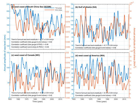
Trends of regional average amplitude of annual sea level in the eight subregions of the North Pacific Ocean derived from long-term tide gauge data in 1952–2014 are presented in Table 3. Statistically significant negative trends were observed in the most areas of marginal seas, with rates of −0.77 mm·yr−1 to −0.11 mm·yr−1. For the rest of coastal areas (ECS, SJ, and JSE), the trends were insignificant (Table 3). For each station, the estimated long-term trends of annual sea level amplitude exhibited geographical non-uniformity (Table 1 and Figure 5). The East Asia tide gauge in the areas of ECS and Japan (SJ, JNE, and JSE) coast showed an inconsistent trend in annual sea level amplitude with a range of −5.3 mm·yr−1 to 6.5 mm·yr−1; the maximum trend of 6.5 mm·yr−1 was obtained from the Shirahama tide gauge data in the JSE coast (Figure 5). In the areas of ECS and Japan coast, the annual sea level variability was strongly influenced by various factors, including atmospheric pressure, wind stress, ocean current, and steric component [10]. Therefore, annual amplitude of sea level cycle in these areas still requires continuous monitoring and analysis to understand the extent of climate change effects on these regions and for disaster prevention.
In the SCSW, the regional average trend of annual sea level amplitude was significantly decreased with a rate of −0.77±0.04 mm·yr−1 for 1952‒2011 (Table 3). A significant decreasing trend was also observed at each station (Table 1 and Figure 5) with a range of −1.15 mm·yr−1 to −0.18 mm·yr−1. In addition, the average mean rate of annual sea level cycle for three subregions of the Northeast Pacific Ocean showed statistically significant negative trends with a range of −0.34 mm·yr−1 to −0.11 mm·yr−1 (Table 3). The changes of annual sea level amplitudes for most tide gauge stations in the Northeast Pacific Ocean showed decreasing trends, except for the positive rate at the Cordova tide gauge in the GA with rate of 0.34±0.07 mm·yr−1 (Table 1 and Figure 5). This discrepancy may be caused by the observations covering different time periods. The time period of Cordova station covers 1964–2016, but the developed EEMD method removes the first and last 2 years from the tide gauge records. Almost no observational data were obtained in 1968–1969, resulting in no observational data before 1970. In the GA, the maximum average annual amplitude (~92 mm) was found in 1952–1969 (Figure 3f), leading to the positive trend at Cordova station. In the following section, we focus on the impact of several factors including steric component, wind stress, and climate indices on the long-term temporal variations of annual sea level amplitude in the areas of SCSW, GA, WC, and WA.
C.C. between tide gauge and altimetry is statistically significant (at 95% confidence level) in each subregion.

5. Discussion

5.1. West Coast of South China Sea

Figure 6 shows the annual cycle amplitude in SCSW that is derived from tide gauges and wind stress and overlaid with the low-pass filtered MEI and PDO. The mean annual sea level cycle amplitude in SCSW decreased significantly from 1952 to 1998, with the smallest amplitude of 115 mm found in 1986–1987. No trend change was observed after 1998. The annual amplitude variability between wind stress and sea level in the SCSW is consistent. The mean annual amplitude of wind stress decreased significantly from 1950 to 1998 but slightly increased after 1998, with a correlation coefficient of +0.62 (Table 4). Cheng et al. [44] indicated that annual sea level variability in the SCSW is dominated by wind forces. The PDO index has an opposite phase to annual amplitude variabilities of sea level and wind stress in the SCSW, which increased significantly from 1950 to 1997, showed the largest index in 1987 and exhibited a slightly decreasing trend after 1997. Comparison between the mean annual amplitudes of sea level and wind stress and PDO index implied that the temporal variations of annual sea level and wind stress amplitudes are negatively correlated with the PDO with the correlation coefficients of −0.48 and −0.46 (Table 4). These results suggested that the changes of annual wind stress in SCSW are associated with PDO [47]. In 1952–2011, the average values of annual sea level amplitude in SCSW decreased significantly. The increases in PDO index prompted the negative trend of the annual amplitude of local monsoon system.

5.2. Eastern Boundary of the North Pacific Ocean

The annual sea level amplitudes of the Northeast Pacific coasts exhibited considerable interannual-to-decadal variability (Figure 7). Those derived from tide gauges along the Northeast Pacific coast (GA, WC, and WA) were correlated with its steric component derived from Ishii data [27] with the correlation coefficients of 0.25–0.51 (Table 4). However, all annual amplitudes of steric component were less than half of the mean annual sea level amplitude derived from tide gauges (Figure 7, Table 2). These differences are partly attributed to the smoothing of the gridded temperature and salinity product and the observations being conducted at different locations. The regional averages of the annual amplitudes of wind stress in the Northeast Pacific coast were highly correlated with the corresponding quantity for the annual sea level amplitude [48] with correlation coefficients of 0.58 for GA, 0.42 for WC, and 0.56 for WA. Since 1980, the two annual amplitudes in the Northeast Pacific coasts have become consistent (Figure 7) with correlation coefficients of 0.61–0.72 compared with those in the period of 1952–1980 (0.25–0.57). This finding indicates that the influence of wind stress field on the annual sea level amplitude varies at different time periods, and the wind field system has a dominant effect on the annual sea level amplitudes in the Northeast Pacific coasts since 1980. Similar results are found for the comparison with altimeter data, with high correlations in the most areas of north Pacific marginal seas [49]. In addition, the annual wind stress and sea level amplitude from 1980 to 2014 showed similar trends in the Northeast Pacific coasts (Figure 7). The weakened annual sea level amplitude of WC and WA for the past 30 years is speculated to be caused by the annual amplitude of wind force manifesting a negative trend.
Wang et al. [50] links the coastal sea level changes to the PDO in the Northeast Pacific Ocean. Comparison between the mean annual sea level amplitude and PDO index revealed that the temporal variations of annual amplitudes in the Northeast Pacific coasts are lowly correlated with the PDO with correlation coefficients ranging from 0 to 0.26 (Table 4). This finding can be attribute to the PDO impact being negligible for the entire period. Hence, the annual sea level amplitude in the Northeast Pacific coasts is not dominated by the PDO. In addition, the variability of annual wind stress amplitude is low correlated with the PDO with correlation coefficients of 0.15 for GA, 0.31 for WC, and 0.31 for WA. This result indicates that PDO did not have a dominant influence on annual amplitude variability during 1952–2014. However, in the Northeast Pacific Coasts, PDO has crucial effects on the changes in other sea level signals (such as sea level trend [51]).

6. Conclusions

The temporal variations of the annual sea level cycle along the North Pacific Ocean coast were investigated by the developed EEMD method using 107 tide gauge records covering the period of 1950–2016. The results showed that average annual sea level amplitudes exhibit interannual-to-decadal variability in the eight subregions and range between 14 and 220 mm. Comparison of the average temporal variations of the annual sea level amplitudes in each subregion for 1952–2014 shows good agreement (R = 0.77–0.85) between the values computed in this analysis and using the TLRA method (with 3-year-long data segment), especially at decadal time scales. The largest mean annual amplitude of 174 mm is found in the SCSW. For the rest of coastal regions, the average annual amplitude is between 77 and 124 mm in the western coast and 84 and 87 mm in the eastern coast. These results agree with the annual amplitude derived by TLRA. The mean difference of annual amplitude between the EEMD and TLRA results is 0 ± 2.6 mm in the eight subregions. Therefore, the EEMD method used in this study can sensitively reflect the annual sea level cycle to obtain a good physical understanding of processes involved in the variation of annual sea level cycle.
The areas of ECS and Japan coast (SJ, JNE, and JSE) are characterized by the estimated long-term trends of annual sea level amplitudes in 1952–2014. An inconsistency in spatial patterns was observed with a range of −5.3 mm·yr−1 to 6.5 mm·yr−1. In these regions, the annual sea level variability is strongly influenced by various factors, including atmospheric pressure, wind stress, ocean current, and steric component [10]. Therefore, their annual amplitudes of sea level cycles still require continuous observation and analysis to understand the extent of climate change effects on these regions.
In the SCSW, the regional average trend of annual sea level amplitude has significantly decreased (−0.77±0.04 mm·yr−1) over 1952‒2011. For each station located in the SCSW, the annual sea level amplitudes present statistically decreasing trends with a range of −1.15 mm·yr−1 to −0.18 mm·yr−1. Steric component has relatively minor impacts on the annual sea level cycle in the SCSW and is estimated to contribute ~42 mm to sea level. This value is less than quarter of the average annual sea level amplitude, which is the smallest contribution of annual amplitude of steric component to the total annual sea level amplitude in the coastal region of the North Pacific Ocean. This difference may be caused by the smoothing of gridded ocean temperature and salinity data, the shallow continental shelf areas, or the poor spatial sampling of Argo floats in the South China Sea [46]. The temporal variation of the annual sea level amplitude is mainly associated with wind stress [44,52], with a correlation coefficient of +0.62. In addition, the PDO index has opposite phases to annual sea level and wind stress amplitudes for the SCSW with the correlation coefficients of −0.48 and −0.46, respectively. We speculated that the weakened local wind system may be associated with the increase in PDO index [44]. The mean annual sea level amplitude from SCSW gradually decreased as a consequence of weakened monsoon system over the past 60 years. The last PDO shift from cold to warm phase occurred in 2014 (Figure 6) [50], leading to high and low sea levels in the Northeast and Northwest Pacific, respectively, in the next few decades [25,53,54].
For the Northeast Pacific Ocean coast (GA, WC, and WA), the temporal variations of average annual sea level amplitude show statistically significant negative trends over 1952‒2014 with a range of −0.34 mm·yr−1 to −0.11 mm·yr−1. Most of the tide gauge stations in the Northeast Pacific Ocean exhibited statistically decreasing trends for their annual sea level amplitudes (Table 1 and Figure 5). The regional mean annual sea level amplitudes derived from tide gauge records are in good agreement with the corresponding wind stress (R = 0.42–0.58), especially with its high correlation with the annual amplitude curves since 1980 (Figure 7) with the correlation coefficients of 0.61–0.72. In addition, annual wind stress and sea level amplitude show similar trends in the Northeast Pacific coasts from 1980 to 2014 (Figure 7). The wind force affecting the annual sea level cycle varies at different time periods and has played a dominant role in the Northeast Pacific coasts since 1980. Furthermore, the annual sea level cycle in the Northeast Pacific Ocean associated with PDO was explored using the tide gauges over 1952–2014. The result indicated that the annual sea level amplitude in the Northeast Pacific coasts is not dominated by the PDO.

Author Contributions

Validation, W.-H.L., C.-Y.K. and H.-C.K.; conceptualization, C.-Y.K. and L.-C.L.; formal analysis, W.-H.L. and H.-C.K.; methodology, W.-H.L. and L.-C.L.; writing–review & editing, C.-Y.K. and H.-C.K.; writing–original draft, W.-H.L.; supervision, C.-Y.K.; investigation, H.-C.K. All authors have read and agreed to the published version of the manuscript.

Funding

This study was funded by the Ministry of Science and Technology of Taiwan (MOST 109-2121-M-019-001- and MOST 109-2222-E-019-001-).

Data Availability Statement

The data presented in this study are available in Lan, W.H.; Kuo, C.Y.; Lin, L.C.; Kao, H.C. Annual Sea Level Amplitude Analysis over the North Pacific Ocean Coast by Ensemble Empirical Mode Decomposition Method. Remote Sens. 2021.

Acknowledgments

The satellite altimeter data were maintained and provided by Archiving, Validation, and Interpretation of Satellite Oceanographic center. We acknowledge the anonymous reviewers.

Conflicts of Interest

The authors declare no conflict of interest.

References

  1. Woodworth, P.L.; Melet, A.; Marcos, M.; Ray, R.D.; Wöppelmann, G.; Sasaki, Y.N.; Cirano, M.; Hibbert, A.; Huthnance, J.M.; Monserrat, S.; et al. Forcing factors causing sea level changes at the coast. Surv. Geophys. 2019, 40, 1351–1397. [Google Scholar] [CrossRef] [Green Version]
  2. Wahl, T.; Calafat, F.M.; Luther, M.E. Rapid changes in the seasonal sea level cycle along the US Gulf coast from the late 20th century. Geophys. Res. Lett. 2014, 41, 491–498. [Google Scholar] [CrossRef] [Green Version]
  3. Tsimplis, M.N.; Woodworth, P.L. The global distribution of the seasonal sea level cycle calculated from coastal tide gauge data. J. Geophys. Res. 1994, 99, 16031–16039. [Google Scholar] [CrossRef]
  4. Dufau, C.; Martin-Puig, C.; Moreno, L. User requirements in the coastal ocean for satellite altimetry. In Coastal Altimetry; Vignudelli, S., Kostianoy, A.G., Cipollini, P., Benveniste, J., Eds.; Springer: Berlin/Heidelberg, Germany, 2011; pp. 51–60. [Google Scholar]
  5. López-García, P.; Gómez-Enri, J.; Muñoz-Pérez, J. Accuracy assessment of wave data from altimeter near the coast. Ocean Eng. 2019, 178, 229–232. [Google Scholar] [CrossRef]
  6. Chen, J.L.; Shum, C.K.; Wilson, C.R.; Chambers, D.P.; Tapley, B.D. Seasonal sea level change from TOPEX/Poseidon observation and thermal contribution. J. Geod. 2000, 73, 638–647. [Google Scholar] [CrossRef]
  7. Vinogradov, S.V.; Ponte, R.M.; Heimbach, P.; Wunsch, C. The mean seasonal cycle in sea level estimated from a data-constrained general circulation model. J. Geophys. Res. 2008, 113, C03032. [Google Scholar] [CrossRef]
  8. Vinogradov, S.V.; Ponte, R.M. Annual cycle in coastal sea level from tide gauges and altimetry. J. Geophys. Res. Oceans 2010, 115, C04021. [Google Scholar] [CrossRef] [Green Version]
  9. Chelton, D.B.; Schlax, M.G.; Samelson, R.M. Global observations of nonlinear mesoscale eddies. Prog. Oceanogr. 2011, 91, 167–216. [Google Scholar] [CrossRef]
  10. Feng, X.; Tsimplis, M.N.; Marcos, M.; Calalfat, F.M.; Zheng, J.; Jorda, G.; Cipollini, P. Spatial and temporal variations of the seasonal sea level cycle in the northwest Pacific. J. Geophys. Res. Oceans 2015, 120, 7091–7112. [Google Scholar] [CrossRef] [Green Version]
  11. Amiruddin, A.M.; Haigh, I.D.; Tsimplis, M.N.; Calafat, F.M.; Dangendorf, S. The seasonal cycle and variability of sea level in the South China Sea. J. Geophys. Res. Oceans 2015, 120, 5490–5513. [Google Scholar] [CrossRef] [Green Version]
  12. Torres, R.R.; Tsimplis, M.N. Seasonal sea level cycle in the Caribbean Sea. J. Geophys. Res. 2012, 117, C07011. [Google Scholar] [CrossRef] [Green Version]
  13. Passaro, M.; Cipollini, P.; Benveniste, J. Annual sea level variability of the coastal ocean: The Baltic Sea-North Sea transition zone. J. Geophys. Res. Oceans 2015, 120, 3061–3078. [Google Scholar] [CrossRef] [Green Version]
  14. Cheng, Y.C.; Xu, Q.; Li, X.F. Spatio-Temporal Variability of Annual Sea Level Cycle in the Baltic Sea. Remote Sens. 2018, 10, 528. [Google Scholar] [CrossRef] [Green Version]
  15. Wu, Z.H.; Schneider, E.K.; Kirtman, B.P.; Sarachik, E.S.; Huang, N.E.; Tucker, C.J. The modulated annual cycle: An alternative reference frame for climate anomalies. Clim. Dyn. 2008, 31, 823–841. [Google Scholar] [CrossRef] [Green Version]
  16. Wu, Z.H.; Huang, N.E. A study of the characteristics of white noise using the empirical mode decomposition method. Proc. R. Soc. Lond. A. 2004, 460, 1597–1611. [Google Scholar] [CrossRef]
  17. Qian, C.; Wu, Z.H.; Fu, C.B.; Zhou, T.J. On multi-timescale variability of temperature in China in modulated annual cycle reference frame. Adv. Atmos. Sci. 2010, 27, 1169–1182. [Google Scholar] [CrossRef]
  18. Bindoff, N.L.; Willebrand, J.; Artale, V.; Cazenave, A.; Gregory, J.; Gulev, S.; Hanawa, K.; Le Quéré, C.; Levitus, S.; Nojiri, Y.; et al. Observations: Oceanic Climate Change and Sea Level. In Climate Change 2007: The Physical Science Basis. Contribution of Working Group I to the Fourth Assessment Report of the Intergovernmental Panel on Climate Change; Solomon, S., Qin, D., Manning, M., Chen, Z., Marquis, M., Averyt, K.B., Tignor, M., Miller, H.L., Eds.; Cambridge University Press: Cambridge, UK; New York, NY, USA, 2007; pp. 385–432. [Google Scholar]
  19. Douglas, B.C. Global sea level rise. J. Geophys. Res. 1991, 96, 6981–6992. [Google Scholar] [CrossRef] [Green Version]
  20. Woodworth, P.L.; Tsimplis, M.N.; Flather, R.A.; Shennan, I. A review of the trends observed in British Isles mean sea level data measured by tide gauges. Geophys. J. Int. 1999, 136, 651–670. [Google Scholar] [CrossRef]
  21. Holgate, S.J.; Matthews, A.; Woodworth, P.L.; Rickards, L.J.; Tamisiea, M.E.; Bradshaw, E.; Foden, P.R.; Gordon, K.M.; Jevrejeva, S.; Pugh, J. New Data Systems and Products at the Permanent Service for Mean Sea Level. J. Coastal Res. 2013, 29, 493–504. [Google Scholar] [CrossRef]
  22. Permanent Service for Mean Sea Level (PSMSL). Available online: http://www.psmsl.org/data/obtaining/ (accessed on 5 March 2018).
  23. Church, J.A.; White, N.J.; Coleman, R.; Lambeck, K.; Mitrovica, J.X. Estimates of regional distribution of sea-level rise over the 1950-2000 period. J. Clim. 2004, 17, 2609–2625. [Google Scholar] [CrossRef]
  24. Kandasamy, S.; Baret, F.; Verger, A.; Neveux, P.; Weiss, M. A comparison of methods for smoothing and gap filling time series of remote sensing observations–application to MODIS LAI products. Biogeosciences 2013, 10, 4055–4071. [Google Scholar] [CrossRef] [Green Version]
  25. Lan, W.H.; Kuo, C.Y.; Kao, H.C.; Lin, L.C.; Shum, C.K.; Tseng, K.H.; Chang, J.C. Impact of Geophysical and Datum Corrections on Absolute Sea-Level Trends from Tide Gauges around Taiwan, 1993–2015. Water 2017, 9, 480. [Google Scholar] [CrossRef]
  26. Amante, C.; Eakins, B.W. ETOPO1 1 Arc Minute Global Relief Model: Procedures, Data Sources and Analysis. In NOAA Technical Memorandum NESDIS NGDC-24; National Geophysical Data Center: Boulder, CO, USA, 2009. [Google Scholar]
  27. Ishii, M.; Fukuda, Y.; Hirahara, S.; Yasui, S.; Suzuki, T.; Sato, K. Accuracy of global upper ocean heat content estimation expected from present observational data sets. SOLA 2017, 13, 163–167. [Google Scholar] [CrossRef] [Green Version]
  28. Steele, M.; Ermold, W. Steric sea level change in the Northern Seas. J. Climate 2007, 20, 403–417. [Google Scholar] [CrossRef]
  29. Kalnay, E.; Kanamitsu, M.; Kistler, R.; Collins, W.; Deaven, D.; Gandin, L.; Joseph, D. The NCEP/NCAR 40-year reanalysis project. Bull. Amer. Meteor. Soc. 1996, 77, 437–472. [Google Scholar] [CrossRef] [Green Version]
  30. Trenberth, K.E.; Large, W.G.; Olson, J.G. The mean annual cycle in global ocean wind stress. J. Phys. Oceanogr. 1990, 20, 1742–1760. [Google Scholar] [CrossRef] [Green Version]
  31. Yang, H.J.; Zhang, Q. On the decadal and interdecadal variability in the Pacific Ocean. Adv. Atmos. Sci. 2003, 20, 173–184. [Google Scholar]
  32. McGregor, S.; Timmermann, A.; England, M.H.; Elison Timm, O.; Wittenberg, A.T. Inferred changes in El Niño–Southern Oscillation variance over the past six centuries. Clim. Past 2013, 9, 2269–2284. [Google Scholar] [CrossRef] [Green Version]
  33. Mantua, N.J.; Hare, S.R.; Zhang, Y.; Wallace, J.M.; Francis, R.C. A Pacific interdecadal climate oscillation with impacts on salmon production. Bull. Am. Meteorol. Soc. 1997, 78, 1069–1079. [Google Scholar] [CrossRef]
  34. Zhang, Y.; Wallace, J.M.; Battisti, D.S. ENSO-like interdecadal variability: 1900–93. J. Clim. 1997, 10, 1004–1020. [Google Scholar] [CrossRef]
  35. Zhang, X.; Church, J.A. Sea-level trends, interannual and decadal variability in the Pacific Ocean. Geophys. Res. Lett. 2012, 39, L21701. [Google Scholar] [CrossRef]
  36. Huang, N.E.; Shen, Z.; Long, S.R.; Wu, M.C.; Shih, E.H.; Zheng, Q.; Tung, C.C.; Liu, H.H. The empirical mode decomposition and the Hilbert spectrum for nonlinear and nonstationary time series analysis. P. Roy. Soc. Lon. A Mat. 1998, 454, 903–995. [Google Scholar] [CrossRef]
  37. Ezer, T.; Corlett, W.B. Is sea level rise accelerating in the Chesapeake Bay? A demonstration of a novel new approach for analyzing sea level data. Geophys. Res. Lett. 2012, 39. [Google Scholar] [CrossRef] [Green Version]
  38. Kong, Y.L.; Meng, Y.; Li, W.; Yue, A.Z.; Yuan, Y. Satellite Image Time Series Decomposition Based on EEMD. Remote Sens. 2015, 7, 15583–15604. [Google Scholar] [CrossRef] [Green Version]
  39. Wang, G.; Chen, X.Y.; Qiao, F.L.; Wu, Z.H.; Huang, N.E. On intrinsic mode function. Adv. Adap. Data Analy. 2010, 2, 277–293. [Google Scholar] [CrossRef]
  40. Huang, N.E.; Wu, M.L.C.; Long, S.R.; Shen, S.S.P.; Qu, W.D.; Gloersen, P.; Fan, K.L. A confidence limit for the empirical mode decomposition and Hilbert spectral analysis. P. Roy. Soc. Lon. A Mat. 2003, 459, 2317–2345. [Google Scholar] [CrossRef]
  41. Wu, Z.H.; Huang, N.E. Ensemble empirical mode decomposition: A noise-assisted data analysis method. Adv. in Adap. Data Analy. 2009, 1, 1–41. [Google Scholar] [CrossRef]
  42. Chambers, D.P. Evaluation of empirical mode decomposition for quantifying multi-decadal variations and acceleration in sea level records. Nonlin. Processes Geophys. 2015, 22, 157–166. [Google Scholar] [CrossRef] [Green Version]
  43. Wu, H.; Kimball, J.S.; Zhou, N.; Alfieri, L.; Luo, L.; Du, J.; Huang, Z. Evaluation of real-time global flood modeling with satellite surface inundation observations from SMAP. Remote Sens. Environ. 2019, 233, 111360. [Google Scholar] [CrossRef]
  44. Cheng, X.H.; Xie, S.P.; Du, Y.; Wang, J.; Chen, X.; Wang, J. Interannual-to-decadal variability and trends of sea level in the South China Sea. Clim. Dynam. 2016, 46, 3113–3126. [Google Scholar] [CrossRef] [Green Version]
  45. Good, S.A.; Martin, M.J.; Rayner, N.A. EN4: Quality controlled ocean temperature and salinity profiles and monthly objective analyses with uncertainty estimates. J. Geophys. Res. Oceans 2013, 118, 6704–6716. [Google Scholar] [CrossRef]
  46. Llovel, W.; Guinehut, S.; Cazenave, A. Regional and interannual variability in sea level over 2002-2009 based on satellite altimetry, Argo float data and GRACE ocean mass. Ocean Dynam. 2010, 60, 1193–1204. [Google Scholar] [CrossRef]
  47. Wu, C.R. Interannual modulation of the Pacific Decadal Oscillation (PDO) on the low-latitude western North Pacific. Prog. Oceanogr. 2013, 110, 49–58. [Google Scholar] [CrossRef]
  48. Sturges, W.; Douglas, B.C. Wind effects on estimates of sea level rise. J. Geophys. Res. 2011, 116, C06008. [Google Scholar] [CrossRef]
  49. Lan, W.H. Assessment of Seasonal-to-Decadal Variability and Trends of Regional Sea Level in the North Pacific Ocean Using Satellite Altimetry and Tide Gauges. Ph.D. Thesis, National Cheng Kung University, Tainan, Taiwan, 2018. [Google Scholar]
  50. Wang, Y.; Liu, H.; Lin, P.; Yin, J. Record-low coastal sea levels in the Northeast Pacific during the winter of 2013–2014. Scientific Reports 2019, 9, 3774. [Google Scholar] [CrossRef]
  51. Bromirski, P.D.; Miller, A.J.; Flick, R.E.; Auad, G. Dynamical suppression of sea level rise along the Pacific coast of North America: Indications for imminent acceleration. J. Geophys. Res. 2011, 116, C07005. [Google Scholar] [CrossRef] [Green Version]
  52. Feng, W. Regional Terrestrial Water Storage and Sea Level Variations Inferred from Satellite Gravimetry. Ph.D. Thesis, Université Toulouse III Paul Sabatier, Toulouse, France, 2014. [Google Scholar]
  53. Strassburg, M.W.; Hamlington, B.D.; Leben, R.R.; Manurung, P.; Lumban Gaol, J.; Nababan, B.; Vignudelli, S.; Kim, K.Y. Sea level trends in Southeast Asian seas. Clim. Past 2015, 11, 743–750. [Google Scholar] [CrossRef] [Green Version]
  54. Hamlington, B.D.; Cheon, S.H.; Thompson, P.R.; Merrifield, M.A.; Nerem, R.S.; Leben, R.R.; Kim, K.Y. An ongoing shift in Pacific Ocean sea level. J. Geophys. Res. Oceans 2016, 121, 5084–5097. [Google Scholar] [CrossRef] [Green Version]
Figure 1. Investigated areas with the tide gauge sites used in this study. Color indicates the length of tide gauge records since 1950. The background was generated based on the global relief model ETOPO1 [26].
Remotesensing 13 00730 g001
Figure 2. Monthly mean sea level variations from Tajiri tide gauge records (blue line) covering 1968–2014 (with IB effect and datum shift corrections) and annual sea level cycles (red line) by ensemble empirical mode decomposition (EEMD) method. Green line and grey line denote the low-frequency components at interannual-to-decadal (intrinsic mode function (IMF) 4 to 5) and multi-decadal (IMF 6 to 8) time scales derived from tide gauge records, respectively.
Remotesensing 13 00730 g002
Figure 3. Temporal variability of mean annual sea level amplitude from tide gauges (TG) and satellite altimetry (ALT) in eight subregions by EEMD (TG-EEMD: grey line; ALT-EEMD: pink line) and TLRA with 3-year-long (TG-TLRA (3 years): red line; ALT-TLRA (3 years): cyan dashed line) and 5-year-long (TG-TLRA (5 years): blue line) data segments shifting month-by-month.
Remotesensing 13 00730 g003
Figure 4. Temporal variability of mean annual sea level amplitude from tide gauges in the East China Sea (ECS). Black line represents monthly sea level variation at Kagoshima II tide gauge in the ECS with IB effect and datum shift corrections. Blue, pink dashed, green, and orange lines represent regional average annual amplitudes derived from tide gauges, satellite altimetry, steric component, and wind stress, respectively.
Remotesensing 13 00730 g004
Figure 5. Estimated trends of mean annual amplitudes derived from tide gauges by EEMD in the Northwest (left panel) and Northeast (right panel) Pacific Ocean. Blank circle indicates the estimates of the trends that are not passing the significance test at 95% confidence level. The background was generated based on the global relief model ETOPO1 [26].
Remotesensing 13 00730 g005
Figure 6. Temporal variability of regional mean annual amplitude along the South China Sea (SCSW) coast derived from (a) tide gauges (blue line) and (b) wind stress (green line) and overlaid with the low-pass multivariate El Niño–Southern Oscillation Index (MEI: grey curves) and Pacific Decadal Oscillation (PDO: orange dashes) covering the time span from 1952 to 2011.
Remotesensing 13 00730 g006
Figure 7. Temporal variability of regional mean annual amplitude along the (a) Gulf of Alaska (GA), (b) west coast of Canada (WC), and (c) west coast of America (WA) coasts derived from tide gauges (blue line), steric component (red dashes), and wind stress (green line) from 1952 to 2014. The purple and yellow dashes denote the trends of annual sea level and wind stress, respectively, over 1980–2014.
Remotesensing 13 00730 g007
Table 1. Trends of annual sea level amplitudes derived from tide gauge records with inverted barometer (IB) and datum shift corrections in the North Pacific Ocean.
AreaNo.NameLat. (° N)Lon.
(° E)
Data PeriodTrend of Annual Sea Level Amplitude (mm yr−1)Completeness (%)
SCSW1Bangkok Bar13.45100.601952–2000−1.15 ± 0.1091
2Ko Sichang13.15100.821952–1999−1.11 ± 0.1094
3Hondau20.67106.801959–2011−0.20 ± 0.07100
4Zhapo21.58111.821961–2014−0.52 ± 0.0999
5Quarry Bay22.29114.211952–2014−0.36 ± 0.0699
6Xiamen24.45118.071956–2002−0.18 ± 0.08100
ECS7Kanmen28.08121.281961–20140.02 ± 0.06 *99
8Mokpo34.78126.381962–20140.18 ± 0.0599
9Jeju33.53126.541966–2014−0.14 ± 0.0699
10Yeosu34.75127.771968–2014−0.07 ± 0.07 *98
11Izuhara II34.20129.291953–20140.18 ± 0.0396
12Sasebo II33.16129.721968–20140.19 ± 0.05100
13Fukue32.70128.851967–2014−0.01 ± 0.06 *98
14Oura32.98130.221967–20140.11 ± 0.0598
15Nagasaki32.74129.871967–20140.09 ± 0.06 *99
16Misumi32.62130.451959–20100.15 ± 0.0597
17Kagoshima31.58130.571959–20140.14 ± 0.0598
18Naha26.21127.671968–20140.17 ± 0.10 *100
SJ19Busan35.10129.041963–2014−0.02 ± 0.05 *99
20Ulsan35.50129.391965–2014−0.15 ± 0.0795
21Mukho37.55129.121967–2014−0.14 ± 0.0597
22Oshoro II43.21140.861952–20140.11 ± 0.02100
23Nezugaseki38.56139.551957–20140.22 ± 0.0590
24Awa Sima38.47139.261968–20140.45 ± 0.0697
25Kashiwazaki37.36138.511957–20140.00 ± 0.05 *95
26Wajima37.41136.901952–20140.15 ± 0.0496
27Mikuni36.25136.151969–20140.23 ± 0.0597
28Maizuru II35.48135.391953–20140.01 ± 0.03 *98
29Tajiri35.59134.321968–20140.00 ± 0.05 *99
30Sakai35.55133.241959–20140.12 ± 0.0397
31Saigo36.20133.331967–20140.15 ± 0.05100
32Hamada II34.90132.071952–20140.16 ± 0.0497
33Mozi33.95130.971960–2006−0.15 ± 0.04100
34Shimonoseki III33.93130.931959–2010−0.26 ± 0.0696
35Hakata33.62130.411967–20140.18 ± 0.05100
JNE36Monbetu II44.35143.371957–2006−0.42 ± 0.0597
37Abashiri44.02144.291970–20140.17 ± 0.0797
38Hanasaki II43.28145.571959–20140.08 ± 0.04 *95
39Kushiro42.98144.371953–2014−0.09 ± 0.0397
40Urakawa II42.17142.771960–2007−0.33 ± 0.0595
41Hakodate I41.78140.721959–20140.03 ± 0.03 *99
42Ominato41.25141.151954–2006−0.13 ± 0.0496
43Asamushi40.90140.861956–20140.02 ± 0.03 *99
44Hachinohe II40.53141.531952–2009−0.10 ± 0.0399
45Miyako II39.64141.981952–20090.02 ± 0.03 *99
46Ayukawa38.30141.511960–20090.00 ± 0.03 *94
47Onahama36.94140.891953–20090.07 ± 0.0399
JSE48Katsuura35.13140.251969–2014−0.05 ± 0.04 *98
49Mera34.92139.831952–20140.01 ± 0.05 *96
50Tiba35.57140.051966–20140.04 ± 0.05 *100
51Yokosuka35.29139.651957–2014−0.23 ± 0.0595
52Aburatsubo35.16139.621952–2014−0.16 ± 0.0399
53Okada34.79139.391967–2014−0.53 ± 0.0799
54Uchiura35.02138.891952–2014−0.39 ± 0.0699
55Shimizu-Minato35.01138.521959–2014−0.37 ± 0.07100
56Maisaka34.68137.611967–2014−0.09 ± 0.10 *99
57Nagoya II35.09136.881959–2014−0.26 ± 0.07100
58Onisaki34.90136.821965–2014−0.09 ± 0.07 *98
59Toba II34.49136.821952–2014−0.35 ± 0.06100
60Owase34.08136.211968–2014−0.08 ± 0.11 *94
61Uragami33.56135.901967–2014−0.27 ± 0.1096
62Kushimoto33.48135.771959–20140.20 ± 0.07 99
63Shirahama33.68135.381968–20140.65 ± 0.09 99
64Kainan34.14135.191955–20140.14 ± 0.07 99
65Wakayama34.22135.151959–20140.27 ± 0.07 99
66Tan-Nowa34.34135.181959–20140.32 ± 0.08 97
67Kobe II34.68135.191959–2014−0.17 ± 0.06100
68Sumoto34.34134.911967–2014−0.14 ± 0.09 *99
69Komatsushima34.01134.591960–20140.30 ± 0.07 99
70Uno34.49133.951959–20140.31 ± 0.07 97
71Takamatsu II34.35134.061959–20140.21 ± 0.05 98
72Matsuyama II33.86132.711959–20140.19 ± 0.06 98
73Kure IV34.24132.551957–20140.15 ± 0.03 98
74Hirosima34.35132.461965–20140.14 ± 0.05 99
75Uwajima II33.23132.551952–20140.09 ± 0.04 99
76Tokuyama II34.04131.81954–20140.16 ± 0.03 100
77Tosa Shimizu32.78132.961959–20140.22 ± 0.06 98
78Hosojima32.43131.671952–20140.15 ± 0.04 97
79Aburatsu31.58131.411959–20140.17 ± 0.06 99
80Odomari31.02130.691967–20140.40 ± 0.11 99
81Nisinoomote30.74130.991967–2014−0.26 ± 0.1099
GA82Seldovia59.44−151.721967–2014−0.23 ± 0.0796
83Seward60.12−149.431966–2014−0.07 ± 0.07 *91
84Cordova60.56−145.751966–20140.34 ± 0.0794
85Yakutat59.55−139.731952–2014−0.23 ± 0.0696
86Sitka57.05−135.341952–2014−0.07 ± 0.05 *99
87Ketchikan55.33−131.631952–2014−0.18 ± 0.0599
WC88Prince Rupert54.32−130.331952–2014−0.01 ± 0.06 *99
89Queen Charlotte City53.25−132.071966–2014−0.31 ± 0.0697
90Bella Bella52.17−128.131963–2014−0.21 ± 0.0797
91Port Hardy50.72−127.481966–2014−0.36 ± 0.0798
92Tofino49.15−125.921952–2014−0.45 ± 0.0696
93Victoria48.42−123.371952–2014−0.44 ± 0.05100
94Vancouver49.28−123.121952–2014−0.28 ± 0.0599
95Point Atkinson49.33−123.251952–2014−0.31 ± 0.0598
WA96Friday Harbor48.55−123.011952–2014−0.41 ± 0.0697
97Neah Bay48.37−124.611952–2014−0.35 ± 0.0597
98Seattle47.60−122.341952–2014−0.34 ± 0.06100
99Astoria46.21−123.771952–20140.12 ± 0.09 *100
100South Beach44.63−124.041969–2014−0.69 ± 0.10100
101Crescent City41.75−124.181952–2014−0.55 ± 0.0598
102San Francisco37.81−122.471952–2014−0.42 ± 0.05100
103Alameda37.77−122.301952–2014−0.45 ± 0.0599
104Port San Luis35.18−120.761952–2014−0.19 ± 0.0594
105Los Angeles33.72−118.271952–2014−0.08 ± 0.04 *99
106La Jolla32.87−117.261952–20140.04 ± 0.04 *92
107San Diego32.71−117.171952–20140.06 ± 0.04 *98
* indicates the estimates of the parameters that do not pass the significance test at 95% confidence level.
Table 2. Mean amplitudes of annual sea level cycle from tide gauges, satellite altimetry, and steric component (0–3000 m) in eight subregions by EEMD and traditional linear regression analysis (TLRA) with 3- and 5-year-long data segments shifting month-by-month.
AreaEEMD (mm)TLRA (mm)
Tide GaugeSatellite AltimetrySteric ComponentTide Gauge
(3-year)
Tide Gauge
(5-year)
SCSW17415342172172
ECS124112107124124
SJ117107112121121
JNE7772698181
JSE10310282102102
GA8749258583
WC8442328280
WA8449328382
Table 3. Trends of mean annual sea level amplitude derived from tide gauges in the eight subregions of the North Pacific Ocean. C.C. refers to correlation coefficient of annual amplitudes between tide gauges and satellite altimetry.
AreaPeriodEEMD
Mean (mm)Trend (mm·yr−1)C.C. with Altimetry
SCSW1952–2011174−0.77 ± 0.040.53
ECS1959–20141240.02 ± 0.04 *0.94
SJ1952–2014117−0.01 ± 0.03 *0.93
JNE1953–201477−0.12 ± 0.020.71
JSE1952–20141030.00 ± 0.04 *0.86
GA1952–201487−0.11 ± 0.040.81
WC1952–201484−0.34 ± 0.040.63
WA1952–201484−0.16 ± 0.040.66
* indicates the estimates of the parameters that do not pass the significance test at 95% confidence level.
Table 4. Correlation coefficient of mean annual amplitudes derived from tide gauges with annual amplitudes from steric component and wind stress, MEI, and PDO. The MEI and PDO indices denote the interannual and decadal variabilities.
AreaSteric ComponentTuTvTuvMEIPDO
SCSW0.270.540.600.62−0.14−0.48
ECS0.670.600.300.41−0.15−0.26
SJ0.60−0.02 *0.260.17−0.05 *−0.17
JNE0.00*−0.16−0.28−0.240.05 *−0.25
JSE0.420.260.290.35−0.15−0.16
GA0.300.650.120.580.220.07 *
WC0.250.380.320.420.220.03 *
WA0.510.420.570.560.390.26
* indicates that the correlations between two variables that do not pass the significance test at 95% confidence level.
Publisher’s Note: MDPI stays neutral with regard to jurisdictional claims in published maps and institutional affiliations.

