
Extraction of Spectral Information from Airborne 3D Data for Assessment of Tree Species Proportions


Abstract
:
1. Introduction
2. Materials
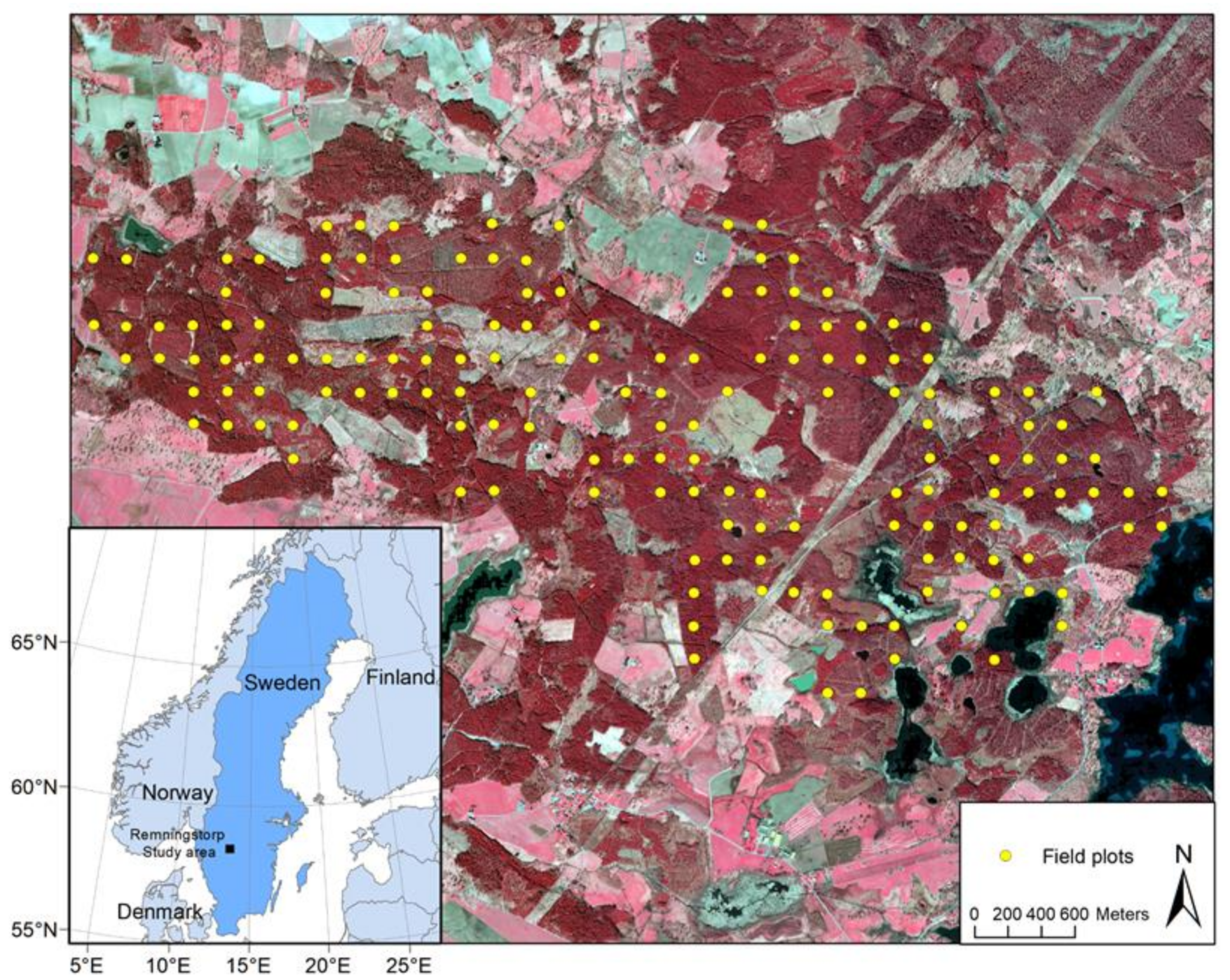
2.1. Study Area
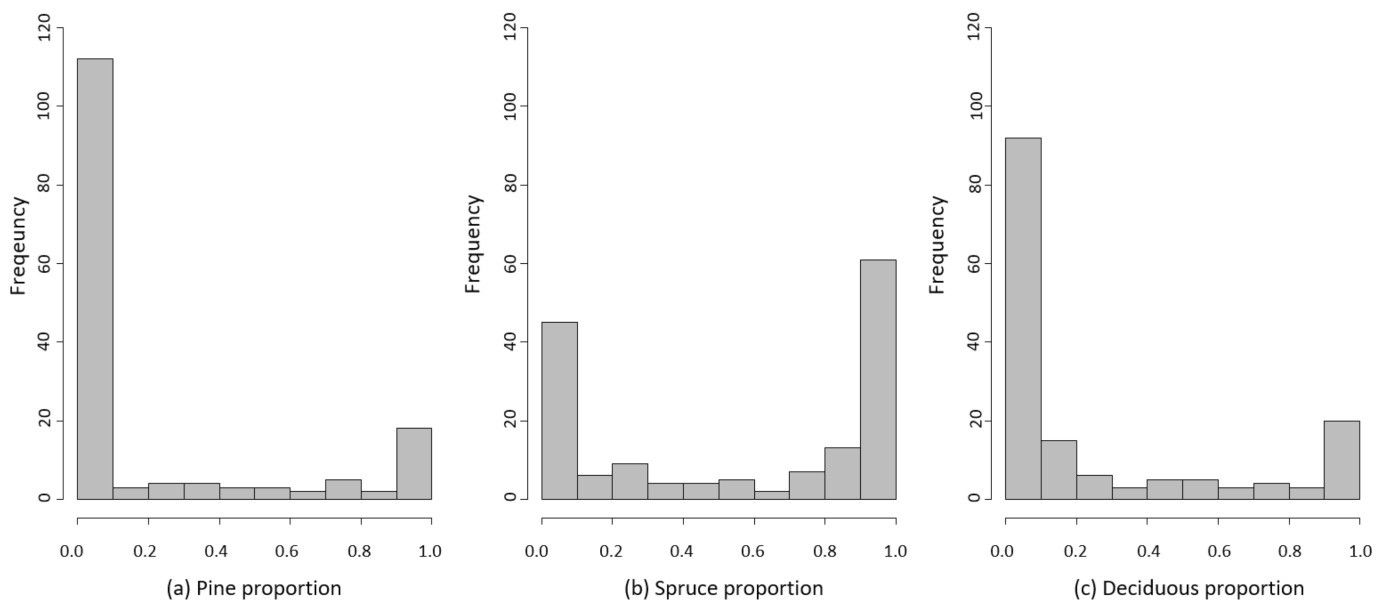
2.2. Field Data
2.3. Aerial Images
2.4. Multi-Spectral Lidar
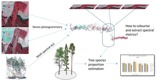
3. Methods
3.1. Stereo Photogrammetry
3.2. Colouring Options
3.3. Spatial Metrics
3.4. Spectral Metrics
3.5. Modelling
3.5.1. Stem Volume
3.5.2. Species Proportion
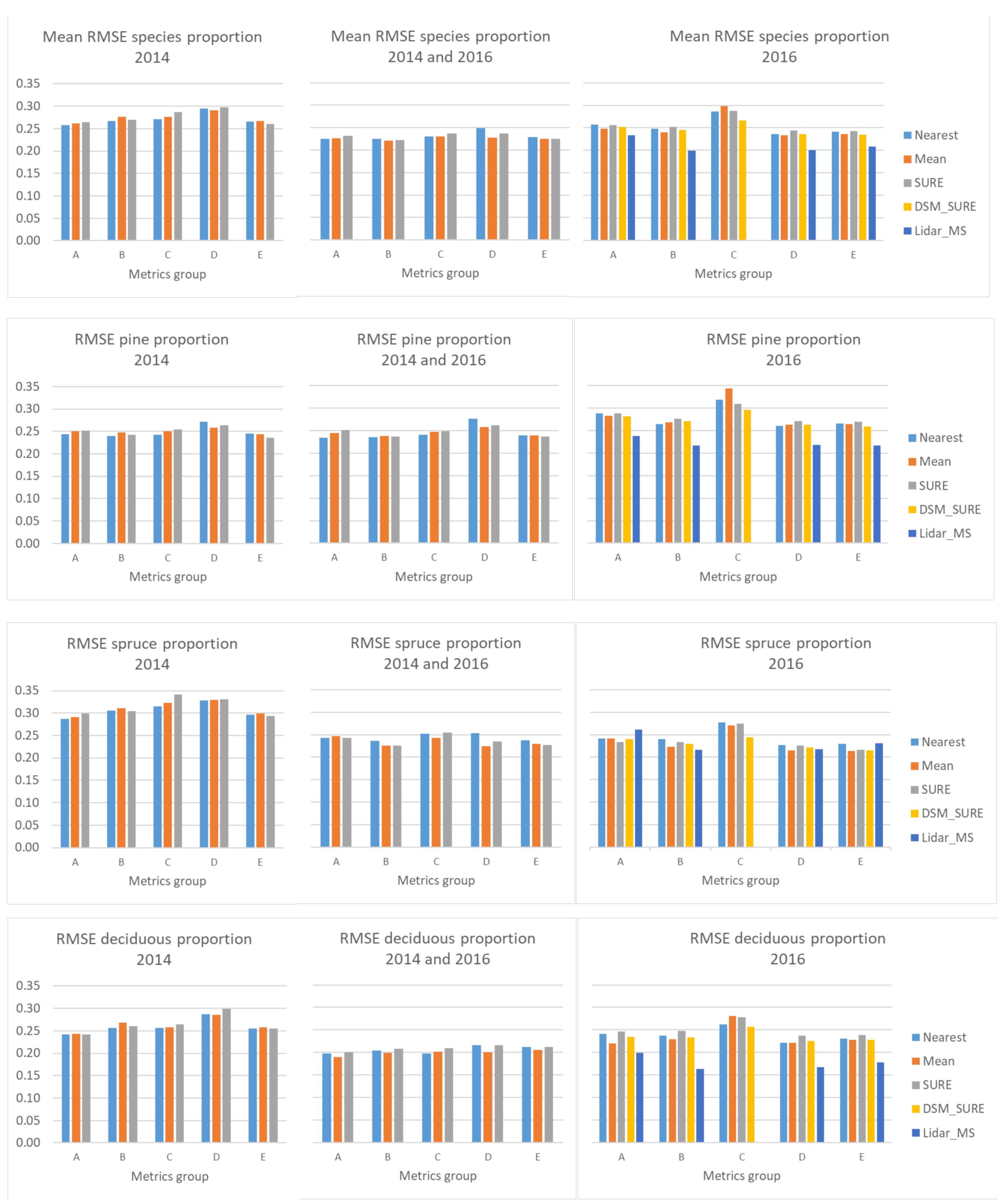
4. Results
5. Discussion
6. Conclusions
Author Contributions
Funding
Data Availability Statement
Acknowledgments
Conflicts of Interest
References
- Magnussen, S.; Boudewyn, P. Derivations of stand heights from airborne laser scanner data with canopy-based quantile estimators. Can. J. For. Res. 1998, 28, 1016–1031. [Google Scholar] [CrossRef]
- Næsset, E. Predicting forest stand characteristics with airborne scanning laser using a practical two-stage procedure and field data. Remote Sens. Environ. 2002, 80, 88–99. [Google Scholar] [CrossRef]
- Næsset, E.; Gobakken, T.; Holmgren, J.; Hyyppä, H.; Hyyppä, J.; Maltamo, M.; Nilsson, M.; Olsson, H.; Persson, Å.; Söderman, U. Laser scanning of forest resources: The Nordic experience. Scand. J. For. Res. 2004, 19, 482–499. [Google Scholar] [CrossRef]
- McRoberts, R.E.; Cohen, W.B.; Næsset, E.; Stehman, S.V.; Tomppo, E.O. Using remotely sensed data to construct and assess forest attribute maps and related spatial products. Scand. J. For. Res. 2010, 25, 340–367. [Google Scholar] [CrossRef]
- Hyyppä, J.; Hyyppä, H.; Leckie, D.; Gougeon, F.; Yu, X.; Maltamo, M. Review of methods of small-footprint airborne laser scanning for extracting forest inventory data in boreal forests. Int. J. Remote Sens. 2008, 29, 1339–1366. [Google Scholar] [CrossRef]
- Packalén, P.; Suvanto, A.; Maltamo, M. A two stage method to estimate species-specific growing stock. Photogramm. Eng. Remote Sens. 2009, 75, 1451–1460. [Google Scholar] [CrossRef]
- Packalén, P.; Maltamo, M. The k-MSN method for the prediction of species-specific stand attributes using airborne laser scanning and aerial photographs. Remote Sens. Environ. 2007, 109, 328–341. [Google Scholar] [CrossRef]
- St-Onge, B.; Budei, B.C. Individual tree species identification using the multispectral return intensities of the Optech Titan lidar system. In Proceedings of the SilviLaser 2015, 14th Conference on Lidar Applications for Assessing and Managing Forest Ecosystems, La Grande Motte, France, 28–30 September 2015. [Google Scholar]
- Kukkonen, M.; Maltamo, M.; Korhonen, L.; Packalen, P. Multispectral airborne LiDAR data in the prediction of boreal tree species composition. IEEE Trans. Geosci. Remote Sens. 2019, 57, 3462–3471. [Google Scholar] [CrossRef]
- Bohlin, J.; Wallerman, J.; Fransson, J.E.S. Forest variable estimation using photogrammetric matching of digital aerial images in combination with a high-resolution DEM. Scand. J. For. Res. 2012, 27, 692–699. [Google Scholar] [CrossRef]
- Gobakken, T.; Bollandsås, O.M.; Næsset, E. Comparing biophysical forest characteristics estimated from photogrammetric matching of aerial images and airborne laser scanning data. Scand. J. For. Res. 2015, 30, 73–86. [Google Scholar] [CrossRef]
- Jarnstedt, J.; Pekkarinen, A.; Tuominen, S.; Ginzler, C.; Holopainen, M.; Viitala, R. Forest variable estimation using a high-resolution digital surface model. ISPRS J. Photogramm. Remote Sens. 2012, 74, 78–84. [Google Scholar] [CrossRef]
- St-Onge, B.; Vega, C.; Fournier, R.A.; Hu, Y. Mapping canopy height using a combination of digital stereo-photogrammetry and lidar. Int. J. Remote Sens. 2008, 29, 3343–3364. [Google Scholar] [CrossRef]
- Goodbody, T.R.H.; Coops, N.C.; White, J.C. Digital aerial photogrammetry for updating area-based forest inventories: A review of opportunities, challenges, and future directions. Curr. For. Rep. 2019, 5, 55–75. [Google Scholar] [CrossRef] [Green Version]
- Puliti, S.; Gobakken, T.; Ørka, H.O.; Næsset, E. Assessing 3D point clouds from aerial photographs for species-specific forest inventories. Scand. J. For. Res. 2017, 32, 68–79. [Google Scholar] [CrossRef]
- Kukkonen, M.; Maltamo, M.; Korhonen, L.; Packalen, P. Comparison of multispectral airborne laser scanning and stereo matching of aerial images as a single sensor solution to forest inventories by tree species. Remote Sens. Environ. 2019, 231, 1–10. [Google Scholar] [CrossRef]
- Heikkinen, V.; Tokola, T.; Parkkinen, J.; Korpela, I.; Jaaskelainen, T. Simulated multispectral imagery for tree species classification using support vector machines. IEEE Trans. Geosci. Remote Sens. 2009, 48, 1355–1364. [Google Scholar] [CrossRef]
- Lillesand, T.; Kiefer, R.W.; Chipman, J. Remote Sensing and Image Interpretation, 6th ed.; John Wiley and Sons: Hoboken, NJ, USA, 2018. [Google Scholar]
- Bohlin, J.; Olsson, H.; Olofsson, K.; Wallerman, J. Tree species discrimination by aid of template matching applied to digital air photos. In Proceedings of the International Workshop on 3D Remote Sensing in Forestry, Vienna, Austria, 14–15 February 2006; Koukal, T., Schneider, W., Eds.; EARSeL SIG Forestry: Münster, Germany; pp. 210–214. Available online: https://boku.ac.at/fileadmin/data/H03000/H85000/H85700/workshops/3drsforestry/Proceedings_3D_Remote_Sensing_2006_rev_20070129.pdf (accessed on 15 February 2021).
- Honkavaara, E.; Arbiol, R.; Markelin, L.; Martinez, L.; Cramer, M.; Bovet, S.; Chandelier, L.; Ilves, R.; Klonus, S.; Marshal, P.; et al. Digital airborne photogrammetry—A new tool for quantitative remote sensing?—A state-of-the-art review on radiometric aspects of digital photogrammetric images. Remote Sens. 2009, 1, 577–605. [Google Scholar] [CrossRef] [Green Version]
- Korpela, I.; Heikkinen, V.; Honkavaara, E.; Rohrbach, F.; Tokola, T. Variation and directional anisotropy of reflectance at the crown scale—Implications for tree species classification in digital aerial images. Remote Sens. Environ. 2011, 115, 2062–2074. [Google Scholar] [CrossRef]
- Xu, Z.; Shen, X.; Cao, L.; Coops, N.C.; Goodbody, T.R.H.; Zhong, T.; Zhao, W.; Sun, Q.; Ba, S.; Zhang, Z.; et al. Tree species classification using UAS-based digital aerial photogrammetry point clouds and multispectral imageries in subtropical natural forests. Int. J. Appl. Earth Obs. Geoinf. 2020, 92, 1–14. [Google Scholar] [CrossRef]
- Honkavaara, E.; Khoramshahi, E. Radiometric correction of close-range spectral image blocks captured using an unmanned aerial vehicle with a radiometric block adjustment. Remote Sens. 2018, 10, 256. [Google Scholar] [CrossRef] [Green Version]
- Nezami, S.; Khoramshahi, E.; Nevalainen, O.; Pölönen, I.; Honkavaara, E. Tree species classification of drone hyperspectral and rgb imagery with deep learning convolutional neural networks. Remote Sens. 2020, 12, 1070. [Google Scholar] [CrossRef] [Green Version]
- Trimble. MATCH-T DSM 6.0 Reference Manual; Trimble INPHO GmbH: Stuttgart, Germany, 2014. [Google Scholar]
- Ulander, L.M.H.; Gustavsson, A.; Dubois-Fernandez, P.; Dupuis, X.; Fransson, J.E.S.; Holmgren, J.; Wallerman, J.; Eriksson, L.; Sandberg, G.; Soja, M. BIOSAR 2010—A SAR campaign in support to the BIOMASS mission. In Proceedings of the 2011 IEEE International Geoscience and Remote Sensing Symposium (IGARSS)—Beyond the Frontiers: Expanding our Knowledge of the World, Vancouver, BC, Canada, 24–29 July 2011; pp. 1528–1531. [Google Scholar] [CrossRef] [Green Version]
- Wikström, P.; Edenius, L.; Elfving, B.; Eriksson, L.O.; Lämås, T.; Sonesson, J.; Öhman, K.; Wallerman, J.; Waller, C.; Klintebäck, F. The Heureka forestry decision support system: An overview. Math. Comput. For. Nat. Res. Sci. 2011, 3, 87–94. [Google Scholar]
- Söderberg, U. Functions for forest management. Height, form height and bark thickness of individual trees. Rapp. Sver. lantbr. Inst. Skogstaxering. 1992, 52. ISSN 03480496. [Google Scholar]
- Wiechert, A.; Gruber, M. UltraCam and UltraMap—Towards all in one solution by photogrammetry. In Photogrammetric Week ’11; Fritsch, D., Ed.; Wichmann: Heidelberg, Germany, 2011. [Google Scholar]
- Rothermel, M.; Wenzel, K.; Fritsch, D.; Haala, N. SURE: Photogrammetric surface reconstruction from imagery. In Proceedings of the LC3D Workshop, Berlin, Germany, 4–5 December 2012. [Google Scholar]
- Hirschmuller, H. Stereo processing by semiglobal matching and mutual information. IEEE Trans. Pattern Anal. Mach. Intell. 2008, 30, 328–341. [Google Scholar] [CrossRef] [PubMed]
- Owemyr, P.; Lundgren, J. Noggrannhetskontroll av Laserdata för ny Nationell Höjdmodell; Högskolan i Gävle: Gävle, Sweden, 2010. (In Swedish) [Google Scholar]
- McGaughey, R.J. FUSION/LDV: Software for LIDAR Data Analysis and Visualization; U.S. Department of Agriculture, Forest Service, Pacific Northwest Research Station, University of Washington: Seattle, WA, USA, 2016. [Google Scholar]
- Korhonen, L.; Morsdorf, F. Estimation of canopy cover, gap fraction and leaf area index with airborne laser scanning. In Forestry Applications of Airborne Laser Scanning; Maltamo, M., Naesset, E., Vauhkonen, J., Eds.; Springer: Dordrecht, The Netherlands, 2014; Volume 27, pp. 397–437. [Google Scholar]
- Vastaranta, M.; Wulder, M.A.; White, J.C.; Pekkarinen, A.; Tuominen, S.; Ginzler, C.; Kankare, V.; Holopainen, M.; Hyyppä, J.; Hyyppä, H. Airborne laser scanning and digital stereo imagery measures of forest structure: Comparative results and implications to forest mapping and inventory update. Can. J. Remote Sens. 2013, 39, 382–395. [Google Scholar] [CrossRef]
- Hijmans, R.J.; van Etten, J.; Mattiuzzi, M.; Sumner, M.; Greenberg, J.A.; Lamigueiro, O.P.; Shortridge, A. Geographic Data Analysis and Modeling: Package “Raster” Version 2016. Available online: https://cran.r-project.org/web/packages/raster/index.html (accessed on 15 February 2021).
- Clark, P.J.; Evans, F.C. Distance to nearest neighbor as a measure of spatial relationships in populations. Ecology 1954, 35, 445–453. [Google Scholar] [CrossRef]
- Ripley, B.D. The second-order analysis of stationary point processes. J. Appl. Probab. 1976, 13, 255–266. [Google Scholar] [CrossRef] [Green Version]
- Bohlin, J.; Wallerman, J.; Fransson, J.E.S. Deciduous forest mapping using change detection of multi-temporal canopy height models from aerial images acquired at leaf-on and leaf-off conditions. Scand. J. For. Res. 2015, 31, 517–525. [Google Scholar] [CrossRef]
- Breiman, L. Bagging predictors. Mach. Learn. 1996, 24, 123–140. [Google Scholar] [CrossRef] [Green Version]
- Breiman, L. Random forests. Mach. Learn. 2001, 45, 5–32. [Google Scholar] [CrossRef] [Green Version]
- Liaw, A.; Wiener, M. Classification and regression by randomForest. R news 2002, 2, 18–22. [Google Scholar]
- R Core Team. R: A Language and Environment for Statistical Computing; R Foundation for Statistical Computing: Vienna, Austria, 2015. [Google Scholar]
- Bohlin, J.; Wallerman, J.; Fransson, J.E.S.; Olsson, H. Species-specific forest variable estimation using non-parametric modeling of multi-spectral photogrammetric point cloud data. In Proceedings of the XXIInd ISPRS Congress, Imaging a Sustainable Future, Melbourne, Australia, 25 August–1 September 2012; Volume XXXIX-B8, pp. 387–391. [Google Scholar]
- Dandois, J.P.; Ellis, E.C. High spatial resolution three-dimensional mapping of vegetation spectral dynamics using computer vision. Remote Sens. Environ. 2013, 136, 259–276. [Google Scholar] [CrossRef] [Green Version]


| Data Set | Data Source | Photogrammetric Product | Colouring Method |
|---|---|---|---|
| UC2014_SURE | 2014 aerial images | SURE point cloud | SURE |
| UC2014_Nearest | 2014 aerial images | SURE point cloud | Nearest images |
| UC2014_Mean | 2014 aerial images | SURE point cloud | Mean of images |
| UC2016_SURE | 2016 aerial images | SURE point cloud | SURE |
| UC2016_Nearest | 2016 aerial images | SURE point cloud | Nearest images |
| UC2016_Mean | 2016 aerial images | SURE point cloud | Mean of images |
| UC2016DSM_SURE | 2016 aerial images | DSM | SURE |
| Lidar2016_MS | 2016 lidar | Multi-spectral lidar | Multi-spectral lidar |
| Group | Metrics | Motivation |
|---|---|---|
| A | minimum, maximum, mean, standard deviation and variance of each spectral band * | fundamental distributional statistics |
| B | mode, covariance, skewness, L-moments (L1, L2, L3, L4), the 1st, 5th, 10th, 20th, 25th, 30th, 40th, 50th, 60th, 70th, 75th, 80th, 90th, 99th percentile and generalized means for the 2nd and 3rd power, of each spectral band | extensive distributional statistics |
| C | mean value of the sunlit part of the CHM for each band and normalised by dividing the value for each band by the sum of all bands | data from the sunlit part only |
| D | groups A, B and C | all spectral metrics |
| E | groups A, B, C and all spatial metrics (see Section 3.3. above) | all spectral and spatial metrics |
| Data Set | Model | RMSE (m3 ha−1) | RMSE (%) |
|---|---|---|---|
| UC2014 | 78.5 | 36.0 | |
| UC2016 | 82.8 | 36.7 | |
| UC2016DSM_SURE | 81.8 | 36.2 | |
| Lidar2016_MS | 82.5 | 36.6 |
Publisher’s Note: MDPI stays neutral with regard to jurisdictional claims in published maps and institutional affiliations. |
© 2021 by the authors. Licensee MDPI, Basel, Switzerland. This article is an open access article distributed under the terms and conditions of the Creative Commons Attribution (CC BY) license (http://creativecommons.org/licenses/by/4.0/).
Share and Cite
Bohlin, J.; Wallerman, J.; Fransson, J.E.S. Extraction of Spectral Information from Airborne 3D Data for Assessment of Tree Species Proportions. Remote Sens. 2021, 13, 720. https://doi.org/10.3390/rs13040720
Bohlin J, Wallerman J, Fransson JES. Extraction of Spectral Information from Airborne 3D Data for Assessment of Tree Species Proportions. Remote Sensing. 2021; 13(4):720. https://doi.org/10.3390/rs13040720
Chicago/Turabian StyleBohlin, Jonas, Jörgen Wallerman, and Johan E. S. Fransson. 2021. "Extraction of Spectral Information from Airborne 3D Data for Assessment of Tree Species Proportions" Remote Sensing 13, no. 4: 720. https://doi.org/10.3390/rs13040720