Article

Application of Remote Sensing Techniques to Discriminate the Effect of Different Soil Management Treatments over Rainfed Vineyards in Chianti Terroir

by
Àngela Puig-Sirera
1,
Daniele Antichi
1,
Dylan Warren Raffa
2 and
Giovanni Rallo
1,*
1
Department of Agriculture, Food and Environment (DAFE), University of Pisa, 80, 56124 Pisa, Italy
2
Institute of Life Sciences, Group of Agroecology, Scuola Superiore Sant’Anna, 56127 Pisa, Italy
*
Author to whom correspondence should be addressed.
Remote Sens. 2021, 13(4), 716; https://doi.org/10.3390/rs13040716
Submission received: 24 November 2020 / Revised: 5 February 2021 / Accepted: 12 February 2021 / Published: 16 February 2021
(This article belongs to the Special Issue Remote Sensing in Irrigated Crop Water Stress Assessment)

Abstract

:
The work aimed to discriminate among different soil management treatments in terms of beneficial effects by high-resolution thermal and spectral vegetation imagery using an unmanned aerial vehicle and open-source GIS software. Five soil management treatments were applied in two organic vineyards (cv. Sangiovese) from Chianti Classico terroir (Tuscany, Italy) during two experimental years. The treatments tested consisted of conventional tillage, spontaneous vegetation, pigeon bean (Vicia faba var. minor Beck) incorporated in spring, mixture of barley (Hordeum vulgare L.) and clover (Trifolium squarrosum L.) incorporated or left as dead mulch in late spring. The images acquired remotely were analyzed through map-algebra and map-statistics in QGIS and correlated with field ecophysiological measurements. The surface temperature, crop water stress index (CWSI) and normalized difference vegetation index (NDVI) of each vine row under treatments were compared based on frequency distribution functions and statistics descriptors of position. The spectral vegetation and thermal-based indices were significantly correlated with the respective leaf area index (R2 = 0.89) and stem water potential measurements (R2 = 0.59), and thus are an expression of the crop vigor and water status. The gravel and active limestone soil components determined the spatial variability of vine biophysical (e.g., canopy vigor) and physiological characteristics (e.g., vine chlorophyll content) in both farms. The vine canopy surface temperature, and CWSI were lower on the spontaneous and pigeon bean treatments in both farms, thus evidencing less physiological stress on the vine rows derived from the cover crop residual effect. In conclusion, the proposed methodology showed the capacity to discriminate across soil management practices and map the spatial variability within vineyards. The methodology could serve as a simple and non-invasive tool for precision soil management in rainfed vineyards to guide producers on using the most efficient and profitable practice.

1. Introduction

Water deficit periods are increasing in frequency and intensity in the Mediterranean basin, due to the higher variation in the amount and distribution of rainfall [1]. Vine trees are one of the most common cultivated woody perennial crops in the Mediterranean region [2], which was traditionally rainfed farmed. Vine growers always seek for a certain level of water stress in vineyards, which is known to increase wine quality [3]. Nonetheless, excessive vine water stress can alter the vegetative growth of vine, yield, berry composition and wine quality. In fact, water is the main constrain for yield in semiarid vineyards [3,4,5]. Therefore, an effective management of the water resource is a priority to alleviate the instability in productivity and negative socioeconomic impacts that the drought phenomena may cause [1].
Continuous tillage and regular soil incorporation of cover crops have been implemented as the most common soil management technique in semiarid vineyards. Many case studies have highlighted the benefits in terms of ecosystem services that an appropriate management of cover crop brings to the vineyard agroecosystem, such as soil protection, improving soil structure and organic matter, water purification and carbon sequestration [6,7,8]. Despite this beneficial effect, farmers are reluctant to grow cover crops as they are perceived as a cause of yield reduction due to nutrients and water competition that may occur between the vine and the cover crop [9,10,11].
In terms of crop water status, cover crops can modify the water balance of the vineyard agroecosystem by increasing transpiration, reducing evaporative water loss and promoting water infiltration, soil storage and holding capacity and crop’s capacity to access soil water [12]. Consequently, the cover crop could increase the agroecosystem resilience to drought phenomena and stabilize vine yield. However, most of the studies carried out on cover crops did not have as the main objective the quantification of the relationship cover crop–crop water supply [12]. Therefore, in order to shift farmers’ perception towards cover crop adaptation, further research is needed, which should focus on a holistic and multidisciplinary approach that assesses the potential ecosystem services that cover crops may provide [5,13].
The use of the multidisciplinary and distributed approach is relevant in viticulture, where the systems are complex with high spatial and temporal variability within and between fields due to the heterogeneity and sparse canopy crop characteristics [14]. Chianti terroir (Tuscany, Italy) is a good example of this complex system, characterized by high variability within its agroecosystems, in terms of soil type and physical properties, topographical aspects, microclimates and landscape complexity [15]. The vineyards are registered under the Controlled Designation of Origin (CDO) Chianti Classico. Dry farming is practiced in Chianti region and promoted by the CDO regulation; however, the increasing water deficit periods make necessary to adopt alternative soil management techniques (e.g., cover crops) and supplemental irrigation, which could be necessary after prolonged drought periods to support the functioning of the vineyard. Hence, monitoring soil and vine water status in relation to soil alternative management practices in Chianti region can represent an innovative practice to support their implementation.
Traditional methods for field data acquisition involve extensive sampling and time-consuming, destructive and discrete measurements, being thus impractical for monitoring large areas and for commercial-scale farming [16,17]. Nonetheless, vineyards are heterogeneous and sparse crop systems with significant intra- and inter-field variability [14]. Remote sensing technology is a valuable tool to study the significant complexity associated to vineyards agroecosystems and more specifically in Chianti region [4]. Among the remote sensing techniques, the unmanned aerial vehicles (UAVs) have become a technology with affordable operational costs, non-invasive, with high spatial and temporal resolution that can be used in commercial vineyards. UAVs are coupled with multispectral and thermal cameras that acquire aerial images of specific spectral responses of the vegetation and thermal infrared region of the spectrum. The images can be processed into vegetation spectral and thermal based indexes that are related to vine biophysical and physiological parameters [18].
UAV thermal infrared images have been widely used to evaluate vine water status variability [19,20]. Canopy temperature is linked to the transpiration cooling effect, as the immediate crop response to water stress is closure of the leaf stomata, which reduces transpiration and consequently increases leaf temperature [21]. Therefore, canopy temperature and thermal based indicators from airborne thermal imaging are used to map spatial variability and quantify crop water status, among which the crop water stress index (CWSI) is one of the most common water stress indices in viticulture. The CWSI was developed as a thermal based stress indicator in herbaceous crops by [22,23] and lately have been used in woody perennial crops [17,24,25]. Spectral vegetation indices have been much studied and have been proved to correlate well with biophysical and physiological vine parameters [26].
The normalized difference vegetation index (NDVI) has been proven to represent crop structural characteristics and vigor, which was correlated to vine water status in environments where soil water deficit is a determinant factor for vine crop [27]. In addition, the ratio between the transformed chlorophyll absorption in reflectance index (TCARI) and the optimized soil-adjusted vegetation index (OSAVI) is a combined spectral index that has been observed to represent accurately physiological vine status, concretely correlated with the chlorophyll a+b content in vegetation. This index removes the soil background effect and non-photosynthetic material that may produce inaccurate results [28,29,30,31].
Moreover, Geographical Information System (GIS) tools paired with UAVs allow rigorous mapping of the variables under study within and between fields and produce quasi-real time maps of vine water status. Therefore, coupling these two tools could assist winegrowers in decision-making processes and in the precision management of alternative soil management techniques.
To the best of our knowledge, few studies [26] have developed an integrated approach to discriminate the effects of different soil management techniques on grapevine water status using remote sensing technologies.
Therefore, the main objective of this paper is to use a combined approach of high-resolution thermal/spectral imagery with GIS tool to discriminate how different soil management practices affect the water status in complex rainfed vineyards from Chianti Terroir (Tuscany, Italy). Specifically, the different soil management treatments were studied in terms of crop water status, vegetation vigor and chlorophyll content. Finally, the cover crop residual effect over the vine row was evaluated through the thermal-based crop water stress index.

2. Materials and Methods

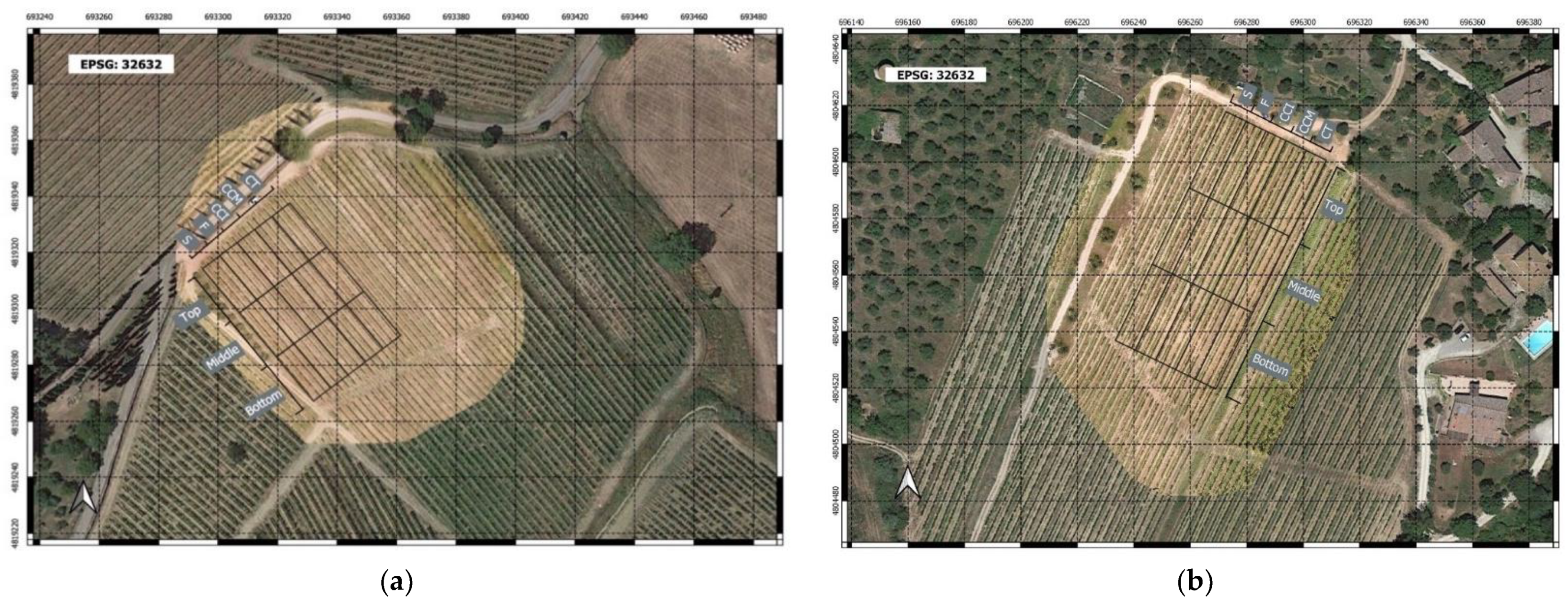
2.1. Study Site Description

The experimental activities were conducted during two seasons (2018–2019) in two organic vineyards within the CDO of Chianti Classico (Tuscany, NW Italy), namely, Fattoria San Giusto a Rentennano (SG) and Azienda Agricola Montevertine (MV). SG farm has an extension of about 160 ha, of which 31 ha correspond to vineyards, while MV sizes 30 ha, of which 18 correspond to vineyards. The experimental plots were planted with the same vineyard variety (Vitis vinifera, L. cvs. Sangiovese R10, rootstock 420A) and same vine and row spacing of 2.50 × 0.8 m2, respectively (5000 vines ha−1). The farms were managed according to the organic farming standards, ordinary soil and canopy management protocols. The vineyards were rainfed to follow the regulation of the CDO Chianti Classico for high quality wines, which enables only supplemental irrigation when needed.
The experimental plot of San Giusto a Rentennano (SG) is localized with geographical coordinates 43°22′05.9″N and 11°25′20.82″E at 233 m elevation above sea level and mean slope of 10%. Average air temperature and annual rainfall account for 14.4 °C and 801 mm, respectively. The extension of the experimental plot was 4000 m2 with North-South row orientation. The vineyards were planted in 1991 and trained according to the guyot system. Soils are loam-clay/loam, developed on ancient fluvial terrace.
The experimental plot of Montevertine (MV) is localized with 43°30′06.1″N and 11°23′28.8″E at 425 m elevation above sea level with a mean slope of 8%. Average air temperature and annual rainfall account for 12.6 °C and 824 mm, respectively. The extension of the plot is 3000 m2 with North-South row orientation. The vineyards were planted in 1995 and trained on spurred cordon trellis system. Soils are stony silty clay loam and clay loam characterized by calcareous flysch of the Monte Morello formation.

2.2. Experimental Design

Table 1 shows the five soil management treatments implemented in both farms, the tillage practices applied under the trellis and inter-row as well as the cover crop management implemented during two seasons.
Each treatment includes three vine rows and two inter-rows (approximately 5 × 100 m), which are separated from the contiguous treatments by one buffer row. The central row of each treatment, used for the remote and ground measurements, was divided into three subplots namely top, middle and bottom, which corresponded to the tophill, middle and valley part of the slope gradient of the experimental plot, respectively (Figure 1).
An in-row ventral plough was used to control weeds under the trellis during the season in all the treatments. The cover crops were sown in October and terminated in mid-June for both experimental years.

2.3. Field Measurements

2.3.1. Soil Physical Characterization

The determination of the soil particle-size distribution was carried out by combining sieving methodology and the novel technique PARIO soil particle analyzer (METER Group, Inc., Pullman, WA, USA). The textural distribution of the soil samples was determined according to USDA classification [32]. Active limestone was determined by the Drouineau method [33].
A total of 15 undistributed soil samples were taken on each farm, which corresponded to three sampling points per treatment, thus one per subplot. On each sampling point, three soil depths were taken: 0–10 cm, 10–30 cm and 30–60 cm. The final results concerned the average data for the entire profile explored (0–60 cm).
The sample positions (Universal Transverse Mercator, UTM, coordinates system) were recorded with a differential GPS (Global Positioning System). Then, the components of the textural analysis were geospatially analyzed using ordinary kriging in the QGIS suite software [34].

2.3.2. Ecophysiological Measurements

The leaf area Index (LAI) was measured by a LAI-2000 optoelectronic sensor (LI-COR, Lincoln, Nebraska, USA), using the two-azimuth protocol for a sparse crop cultivated in rows [35]. The LAI measurements were carried out in the period of maximum vegetative development of the vineyard and were paired with the NDVI computed on the base of the images acquired by UAV on 03 August 2018. First, the sensor was positioned above the vine canopy to perform an ambient light standardization (type A measurement). Seven under-canopy measurements were taken along a diagonal transect pointed toward the middle of the interrow of each soil management treatment, with the instrument held a few centimeters above the soil (type B measurements). Thus, the LAI measurements were implemented through two repetitions of the ABBBBBBB acquisition sequence on each treatment. This procedure was repeated for a total of two transects per soil management treatment in order to investigate both sides of the central vine row of the investigated treatments. The localization of the transect was selected in order to cover the maximum spatial variability of the vigor. A physical cap was used to limit the azimuthal field-of-view to 180°, facing away from the operator and the adjoining row of vines. The measurements were performed when sunlight was low. in order to avoid the direct sunlight influence.
The SPAD readings were performed in both farms in June and August 2018, closed to the day where the NDVI and TCARI/OSAVI images were acquired. To this scope, a portable chlorophyll meter SPAD Minolta 502D has been used. Five rootstocks were selected per subplot, thus a total of 15 plants per treatment. In each plant, three shoots were selected, and SPAD was measured on three fully expanded median leaves. Three readings were taken and averaged on each leaf. This protocol allowed to obtain representative values of the chlorophyll content at canopy scale.
Measurements of midday steam water potential (MSWP) were performed in both farms in July 2019, next to the day where the thermal images were acquired. In particular, a delay of three days occurred between the MSWP and UAV acquisitions, and no substantial variation in water status was observed during those days due to the stable soil drying conditions. Practically, the measurements of MSWP were acquired with a Scholander pressure chamber (PMS Model 600, Albany, OR, USA) according to the precautions suggested by [36]. The measurements were performed between 12:00and 14:00, and two hours previous to the measurement, the leaves were covered in aluminum foil bags to reach the water status equilibrium between leaf and stem. The determinations were carried out in one healthy mature leaf per vine, which was exposed to direct solar radiation. A total of nine plants were measured per treatment (e.g., three plants per subplot), thus fourteen plants on each farm.

2.4. Remote Sensing Measurements

The spectral and thermal radiometric measurements were addressed to acquire the reflectance in the red and infrared bands to calculate the vegetation (i.e., NDVI, TCARI/OSAVI) and thermal (CWSI) indexes.

2.4.1. UAV Platform and Setting

The multispectral and thermal measurements were carried out with an unmanned aerial vehicle (UAV) consisting of a counter-rotating coaxial bladed hexacopter Zephyr EXOS. The UAV was mounted with a multi-spectral sensor Parrot Sequoia (Parrot SA) and a thermal camera FlirVuePro R 640 13mm (FLIR, USA). The multi-spectral sensor acquired four multispectral bands in the green (G), red (R), red edge (RE) and near-infrared (NIR) domain with the respective spectral band width of 530–570 nm, 640–680 nm, 730–740 nm and 770–810 nm. The thermal camera measurement accuracy is +/−5 °C or 5% of reading.
The multispectral camera was equipped with a fully integrated sunshine sensor for in situ calibration of the solar lighting conditions at the time of acquisition. The flight survey was set at 30 m above ground level (AGL) at solar noon, thus producing a Ground Sampling Distance (GSD) equal to 2.82 cm pixel−1 image resolution, which is considered suitable for both thermal surface and vegetative analysis.
The waypoint route was developed to obtain 85% overlap both between photos (forward overlap) and between flight lines (lateral overlap), in order to achieve the highest accuracy in the mosaicking elaboration step. The images were geo-referenced using relevant points on the image such as field corners or obvious end of row. The UAV flights were performed during homogeneous and stable radiation conditions, under sunny, clear sky, no wind and dry soil conditions.
Three drone flights were planned considering the periods of fruit set and full development of the crop. The first two flights were carried out in 2018 (16 June and 27 July) to estimate the NDVI and TCARI/OSAVI indexes, while the third flight was performed in 2019 (03 August) to estimate the surface temperature and the CWSI. In 2019, a thermal image of the surface temperature on a small lake near MV farm was acquired in order to calibrate the thermal image.

2.4.2. Spectral and Thermal Images Processing

The multispectral and thermal images acquired by the UAV were processed using the Pix4D photogrammetry software to develop reflectance maps, vegetation indexes (NDVI, TCARI/OSAVI), thermal and crop water stress index maps. All images were orthorectified, corrected for geometric errors and calibrated radiometrically.
The visible map (RGB) allowed to frame the study area and to observe qualitatively the vegetation density. The vegetation indices used to generate information about biophysical characteristic of the canopy were the NDVI [37] and the TCARI/OSAVI [28,38]. Moreover, the thermal analysis used directly the surface temperature images to compute the CWSI [23].
The method described in [39] was used to calculate the CWSI, which uses an analytical approach to determine Twet (i.e., temperature of the crop without water stress) and Tdry (i.e., temperature of the crop at maximum water stress) based on the frequency of distribution of pure canopy vine temperatures pixels after removing the soil background effect. Twet corresponds to the average temperature of the 0.5% values on the left side of the vine canopy temperatures histogram (i.e., lowest canopy temperatures), and Tdry corresponds to the average temperature of the 0.5% values on the right side of the histogram (i.e., highest canopy temperatures).

2.5. Data Mapping and Analysis

The vegetation and thermal indexes and the georeferenced data collected in the field (e.g., soil texture, MSWP, LAI, SPAD) were managed through open-source GIS technology: QuantumGIS (QGis). The extraction of the vegetation and thermal indexes values that correspond to the vine canopy pixels were performed following two ways using QGIS software. First, the vine row pixels of the NDVI, TCARI/OSAVI and surface temperature images were extracted by drawing a polygon mask that took into account only the central vine row (plant + soil background) of each soil management treatment. The polygon size and length were fixed and designed to accurately identify each vine central row, which was possible due to high spatial resolution of the images [40]. At the same time, each polygon was split in three sub-polygons with the same size that correspond to the treatment subplots (e.g., top, middle and bottom). The raster images of each spectral and thermal indexes were clipped with the polygon and the subplots of the central vine row. Then, the clipped raster image was transformed into a vector layer, from which the point values of the vine canopy pixels were extracted.
In the second way, the plugin i.segment with thresholding method in QGIS was used to extract the pixels values that corresponded solely to the vine crown [41], thus eliminating the soil and mixed pixels. This plugin was used in the surface temperature images in order to calculate the CWSI refereed to the vine rows.
The statistical analysis was carried out using Prism 9 (© 2020 GraphPad Software). The spectral vegetation and thermal pixels were assessed by studying their relative distribution frequency. The statistics descriptors of position (minimum, 1st quartile, median, 3rd quartile and maximum) of the pixels correspondent to the central vine row were determined. One-way ANOVA and multiple comparison pairwise test (Tukey’s test, α = 0.05) were used in the CWSI to discriminate the treatments, whereas simple regression analysis was carried out to determine an empirical relationship between the remote sensing data and field measurements.

3. Results

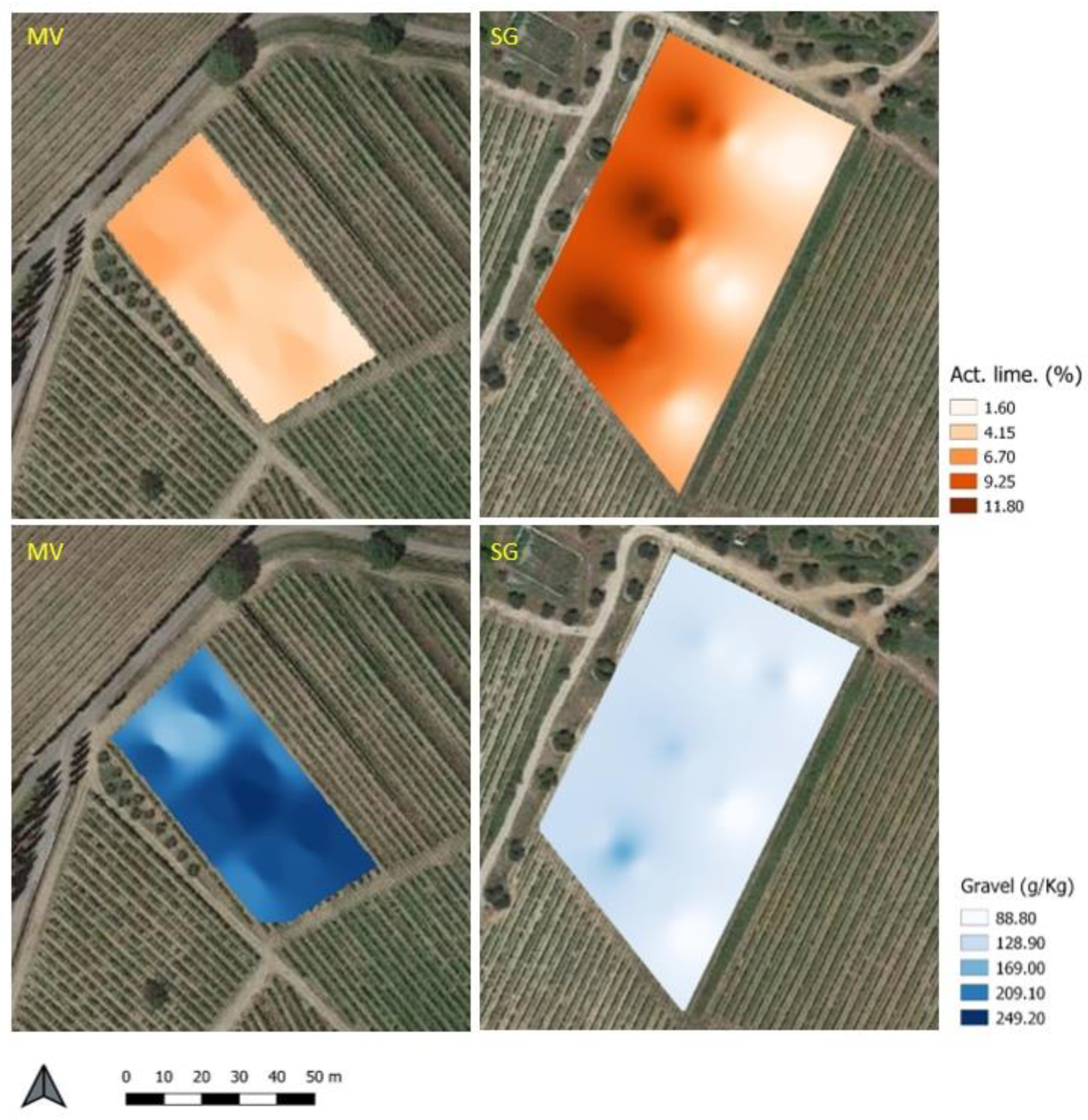
3.1. Soil Physical Properties

Table 2 shows the content percentages of clay, silt, sand and active limestone, as well as the gravel content (g Kg−1) in the soils of the two farms. The fine components (clay, silt and sand) were comparable between the two farms, while the content in gravel was on average higher in MV. The soils of SG, on the other hand, presented a higher percentage of active limestone. According to the USDA [32], classification of soil textural class, both for SG and MV, was distributed between the clay-loam (CL) and silty-loam (SiL) textural classes [32].
The thematic maps for active limestone and gravel (Figure 2), respectively for MV and SG farms, show that for SG, there was a gradient both for the gravel and active limestone, which are more concentrated in the North-West zone and then degrade towards the South-East. On the other hand, MV did not present homogeneous gradients, but rather a wider variability of the distribution of the gravel, which was more concentrated in the middle (reaching contents of 227–250 g kg−1) and less on the upper part of the experimental field. Moreover, the percentage of active limestone was higher in the upper part and diminishing in the lower part of the field.

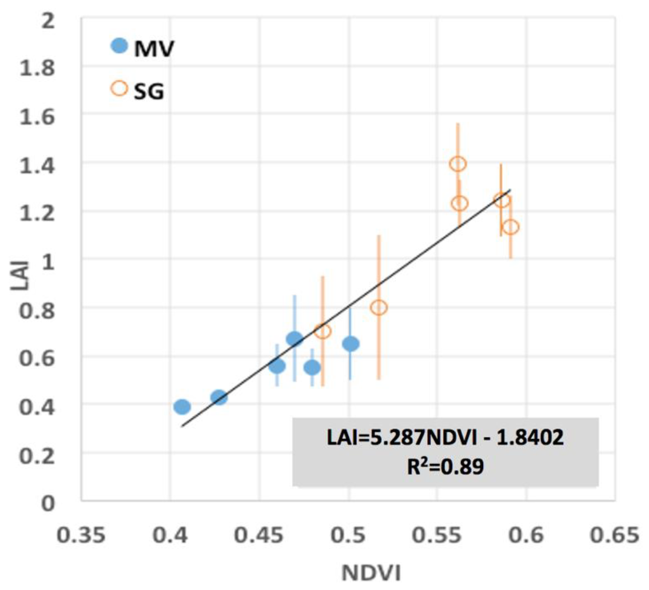
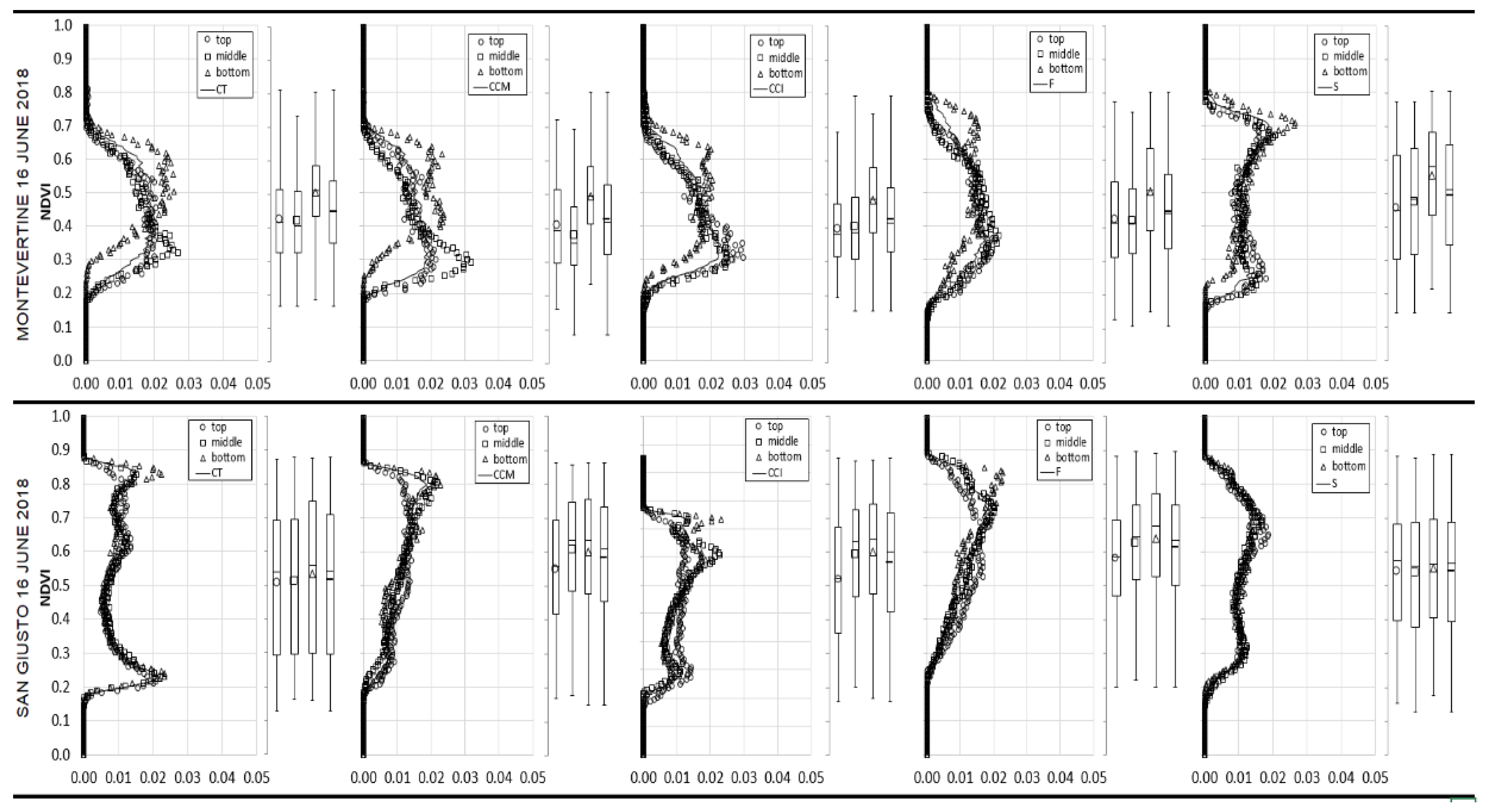
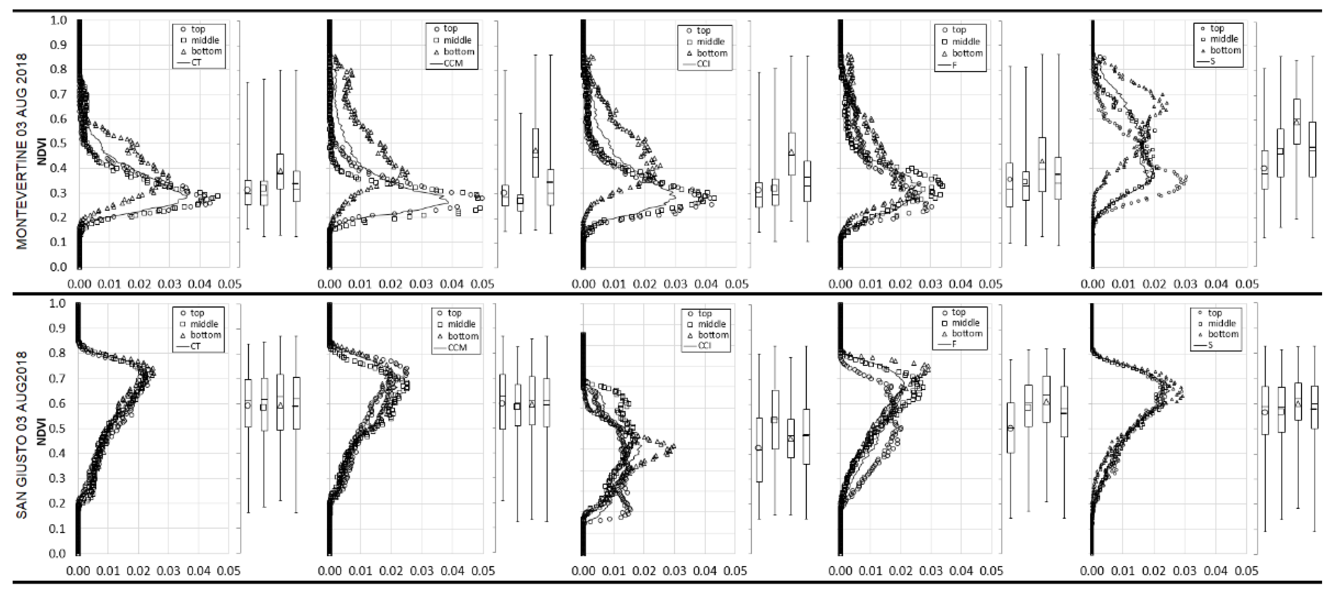
3.2. Structure of the Vegetation Spectral Variability

Figure 3 shows the correlation between the NDVI and the corresponding LAI measurements in each farm. There is a strong correlation between the NDVI and the LAI measurements (R2 = 0.89) at the veraison vine stage in both farms. The vertical bars represent the variability of the LAI measurement expressed in terms of standard deviation. The LAI values and its variability were higher in the vineyards of SG (1.8 ± 0.25 m2 m−2) than in MV (0.55 ± 0.12 m2 m−2).
The LAI and NDVI measurements of the two farms were aligned on the same regression line, which means that the NDVI was influenced by the structure of the vineyard surface, such as the canopy architecture and leaf orientation. Moreover, the alignment in the same line confirms that the vineyards surface characteristics were similar in the two farms: same vine variety, canopy and soil management.
Figure 4 shows the NDVI spatial distribution recognized for the two farms. The NDVI maps evidenced a different structure of the canopy vigor for each flight in each experimental farm. First, the different vigor structure of the two flights was likely related to the different degree of development of the vine crop. In June, the vineyard was at the fruit setting, while in August the vineyard can be considered mature with a fully developed foliage at the veraison stage.
The spatial patterns of the NDVI are more stable when the vine crop is fully developed, thus at veraison stage. Therefore, there was a gradient of the NDVI from North-West to South-East at SG farm. This gradient may depend on the combined action of two soil chemical-physical properties: gravel and active limestone content. Both were more concentrated in the North-West zone and then degraded towards the South-East, as was evidenced previously in the soil physical analysis.
On the other hand, the NDVI did not present a homogeneous gradient in MV but a widespread variability also linked to the distribution of the gravel content. Therefore, the rows appeared more vigorous in the north-corner area of the plot, where a lower gravel content was concentrated. Conversely, the higher gravel content (227−250 g kg−1) at the central part of the plot induced less vigorous canopies.
Referring the two UAV flights, Figure 5 and Figure 6 depict the distribution frequency of the NDVI pixels, which are referred to the central vine row of the treatment and for the three subplots (e.g., top, middle and bottom) localized along the slope gradient. The same Figures also show the boxplots that allow a quick encoding of the distribution frequency.
The bimodal shape of the distribution frequency is typical of sparse crops such as vineyards. The bimodal behavior of NDVI, as described in [42], is related to the soil background effect always present in heterogeneous sparse crops, which do not cover completely the soil. The first mode was located at about NDVI ≈ 0.3, in both farms, and reflects the soil contribution, while the values higher than 0.3 concern soil-vegetation mixed pixels (i.e., transition zone) and crop vegetation. Therefore, the target corresponding solely to the vine vegetation had higher NDVI values, which were situated on the second mode of the distribution frequency.
In MV, the bottom part of the vine row appeared on average more vigorous than in the middle and top slope gradient. The S treatment depicted more vigor compared to the other treatments, both in the June and August flight (NDVI ≈ 0.5). There was a decrease in the vine vigor on August, except for the S treatment. Hence, the first mode of the distribution frequency was smoother for F, followed by CCM, CCI and CT treatments.
Regarding SG farm, the vine vigor followed the slope gradient, though this trend was weaker with respect to MV. As discussed for MV, in August the vines depicted lower vigor values than in June in all treatments. Specifically, the CT treatment exhibited a more marked pick of the first mode in June; thus, there was higher soil incidence, which could be caused by lower canopy vigor.
Figure 7 shows the TCARI/OSAVI spatial distribution acquired with the two flights. The same vigor spatial patterns that were observed previously for the NDVI images could be appreciated in the TCARI/OSAVI spatial distribution at the veraison stage in both farms. Thus, the NDVI and TCARI/OSAVI indexes could depict an analogous gradient in terms of vegetative vigor, chlorophyll concentration and efficiency of the photosynthesis, which were correlated to the gravel and active limestone concentrations in the soil.
The SPAD measurements were plotted against the correspondent TCARI/OSAVI values acquired in both flights (Figure 8). Moreover, the graph includes gravel content, which is proportional to the size of the bubble. There was a negative linear correlation (R2 = 0.60) between the two variables. The values of TCARI/OSAVI were higher in June than in August for both farms, probably due to the mature condition of the leaf structure at the veraison stage. However, the relationship represents the TCARI/OSAVI patterns in time but not in space, which could be related to the limited number of measurements at leaf level that did not allow a good interpretation of the intra-field variability of the SPAD.

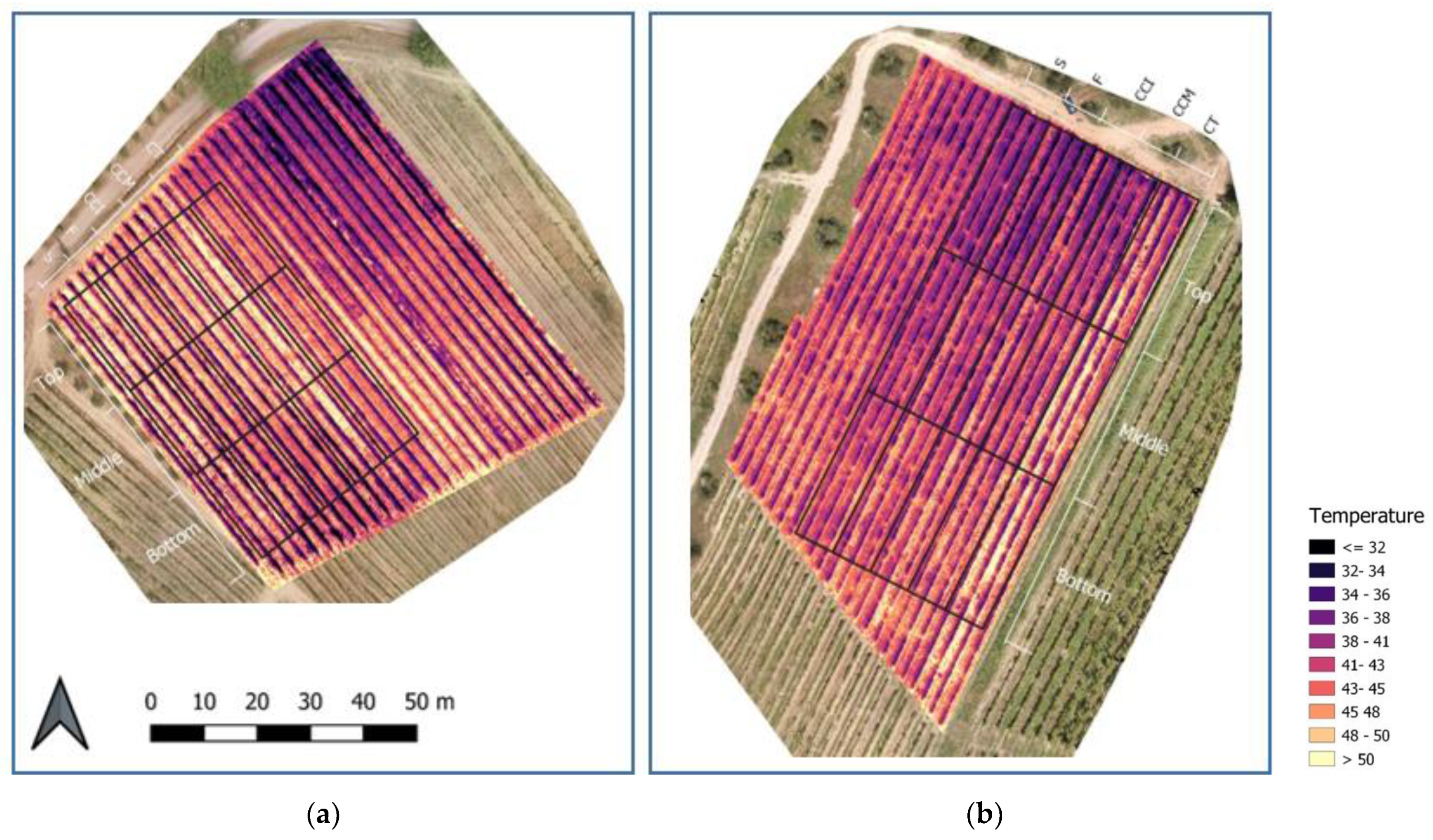
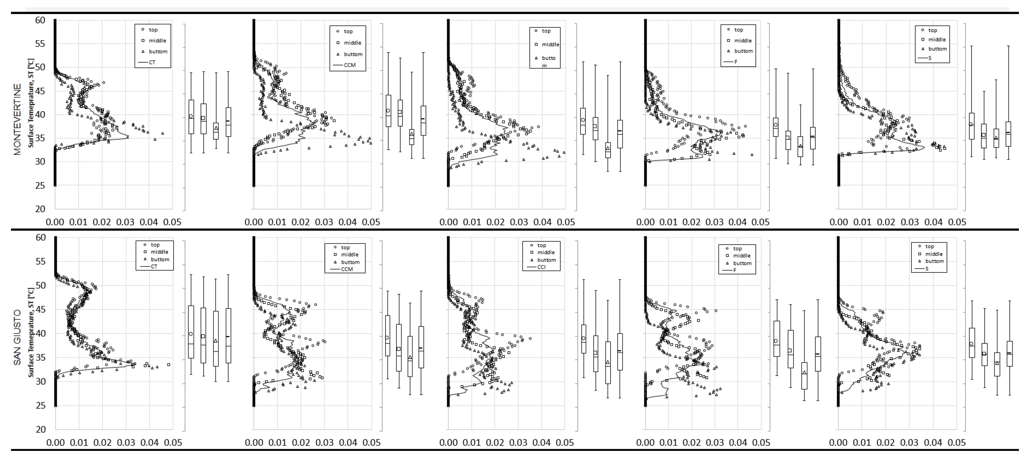
3.3. Structure of the Surface Temperature Variability

The thermal analysis used the surface temperature images provided by the drone flight on the 27 of July 2019, when we hypothesized that a cover crop residual effect of the different soil management treatments can be observed over the vineyards water status.
The air temperature and humidity at the time of the drone flight were 29 °C and 30% in MV and 32 °C and 40% in SG, respectively. The water body temperature measured with a handheld infrared thermometer was equal to 30°C, which was the same to the one registered by the UAV thermal image. Therefore, this process allowed validating the thermal image acquired by the UAV [24,43,44]. MV and SG farms are situated in the same latitude and presented similar atmospheric conditions at the time of the image acquisition; hence, we can consider that water body temperatures could be a reference value of the minimum thermal status of the two agro-environments.
Figure 9a,b shows the spatial distribution of the surface temperatures referred to the whole experimental plots. Analyzing the images, we could identify a similar visual pattern of the spatial variability to the one described above for the NDVI and TCARI/OSAVI indexes at the veraison stage. Consequently, the surface temperature was affected by the surface radiative properties (i.e., albedo and emissivity), which were linked to the canopy surface and the soil background distributions. MV did not present a homogeneous gradient of the spatial distribution of temperatures, but lower temperatures can be found in the bottom part of the plot, which corresponds to the valley part, where the soil water content would be higher than in the upper part.
As discussed for the NDVI, the distribution frequencies of the surface temperatures were bimodal, in which two modes represented the vegetation and soil effects (Figure 10). The first mode was positioned in the lower part of the graph and hence lower temperatures corresponding to the vine canopy and the second mode in the upper part with higher temperatures, which refers to the soil background.
In both farms, the CT treatment presented more marked bimodal distribution with the first mode around 33.5° and the second one at 48.7° in SG, whereas in MV were 35.0 °C and 46.0 °C, respectively. Therefore, there was a soil background effect that imposes a higher incidence of the soil thermal contribution on CT compared to the other treatments. Contrarily, the second mode was not present in the S treatment, which suggests that the S treatment was more vigorous compared to the others. Moreover, the presence of the spontaneous vegetation during the entire season could reduce the sensible heat flux (H) that would affect the nearest vine row [45], which was the opposite in the other treatments where the cover crop vegetation was removed at specific times.
In MV, the soil background effect was more important according to these series: CT > CCM > CCI > F > S. This is shown by the sharpest peak of the second mode; thus, the more marked the peak, the more incidence of the soil in the treatment studied. The lower soil incidence in the soil management techniques was verified with the highest values of the NDVI. The soil modes identified among the treatments were more marked in SG than MV farm.
The median and quartiles of every distribution frequency in both farms follow the slope gradient. Hence, the bottom part had a lower temperature in all treatments in both farms, which is in line with [40], a study that highlighted vine water status dependent on the plot slope. As a consequence, there is a combined slope-soil properties effect which could affect the crop thermal status.

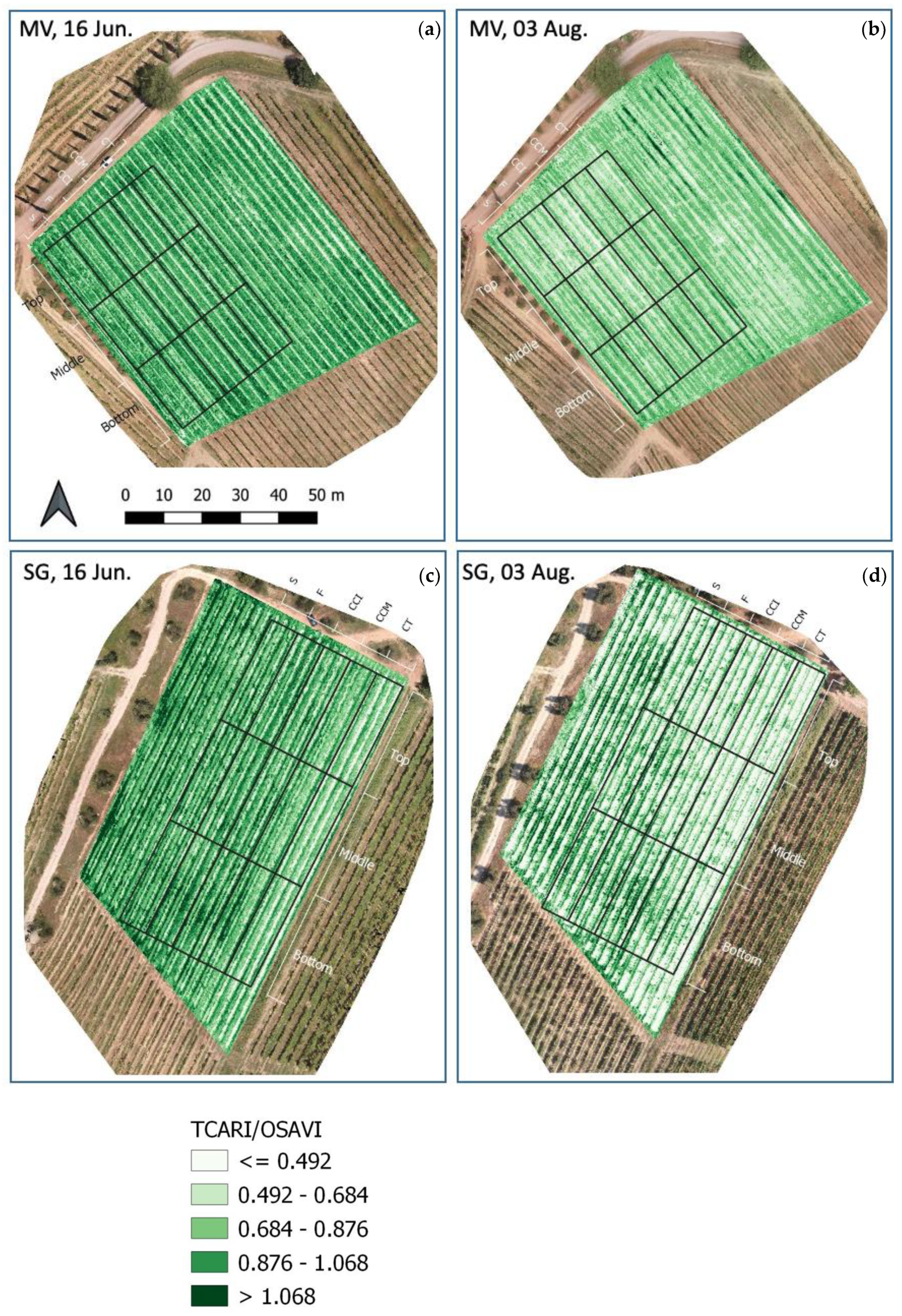
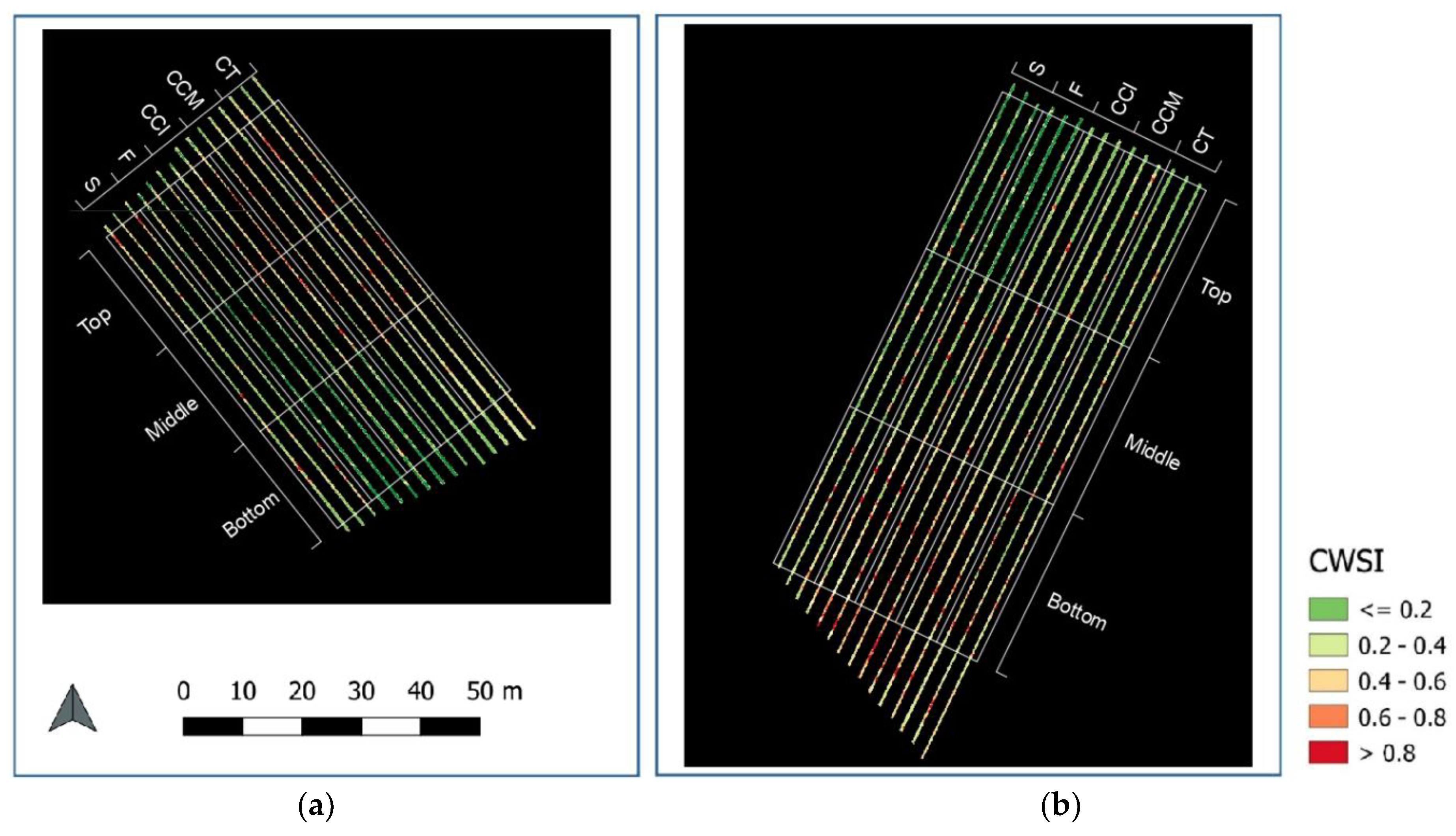
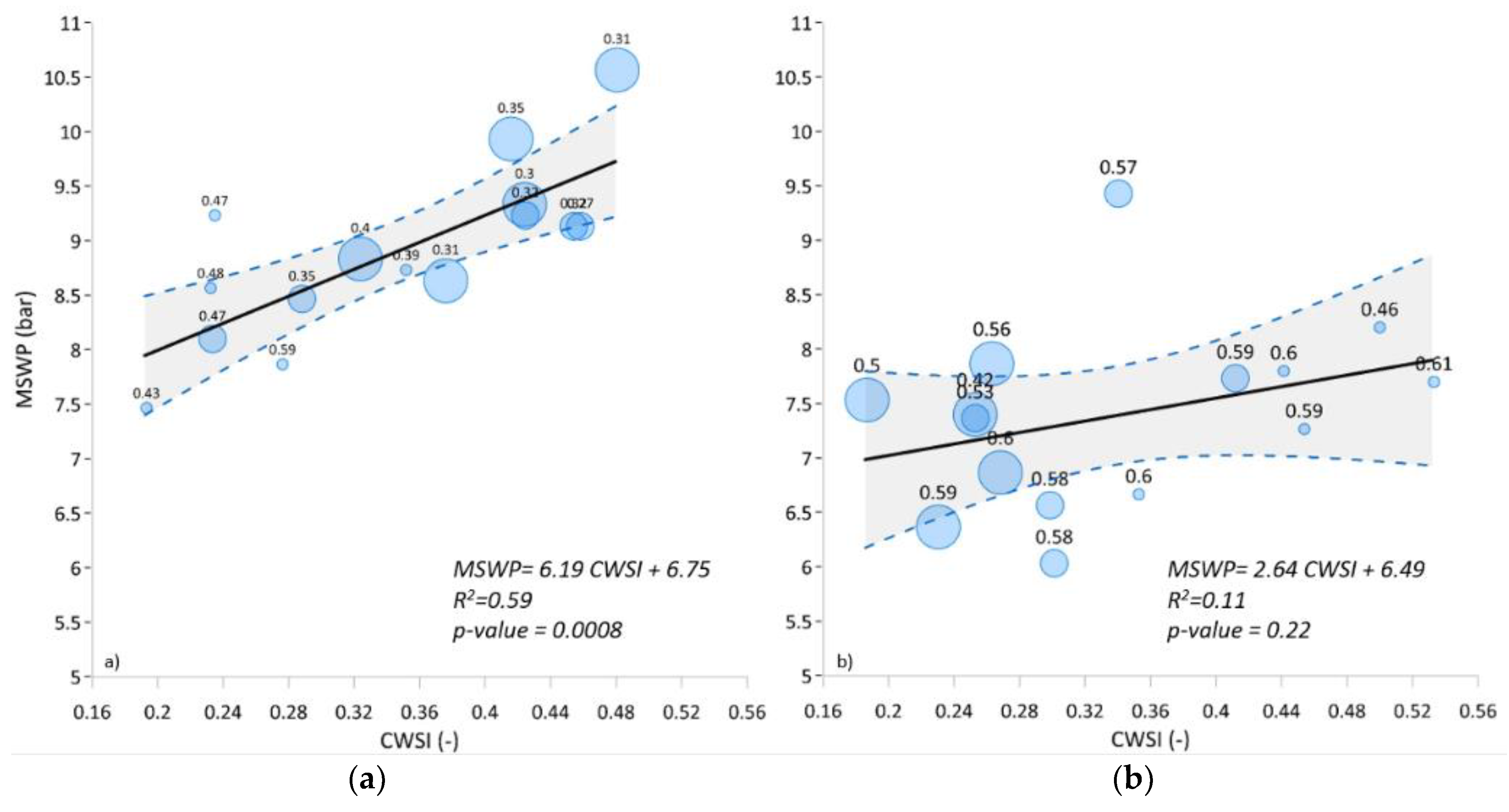
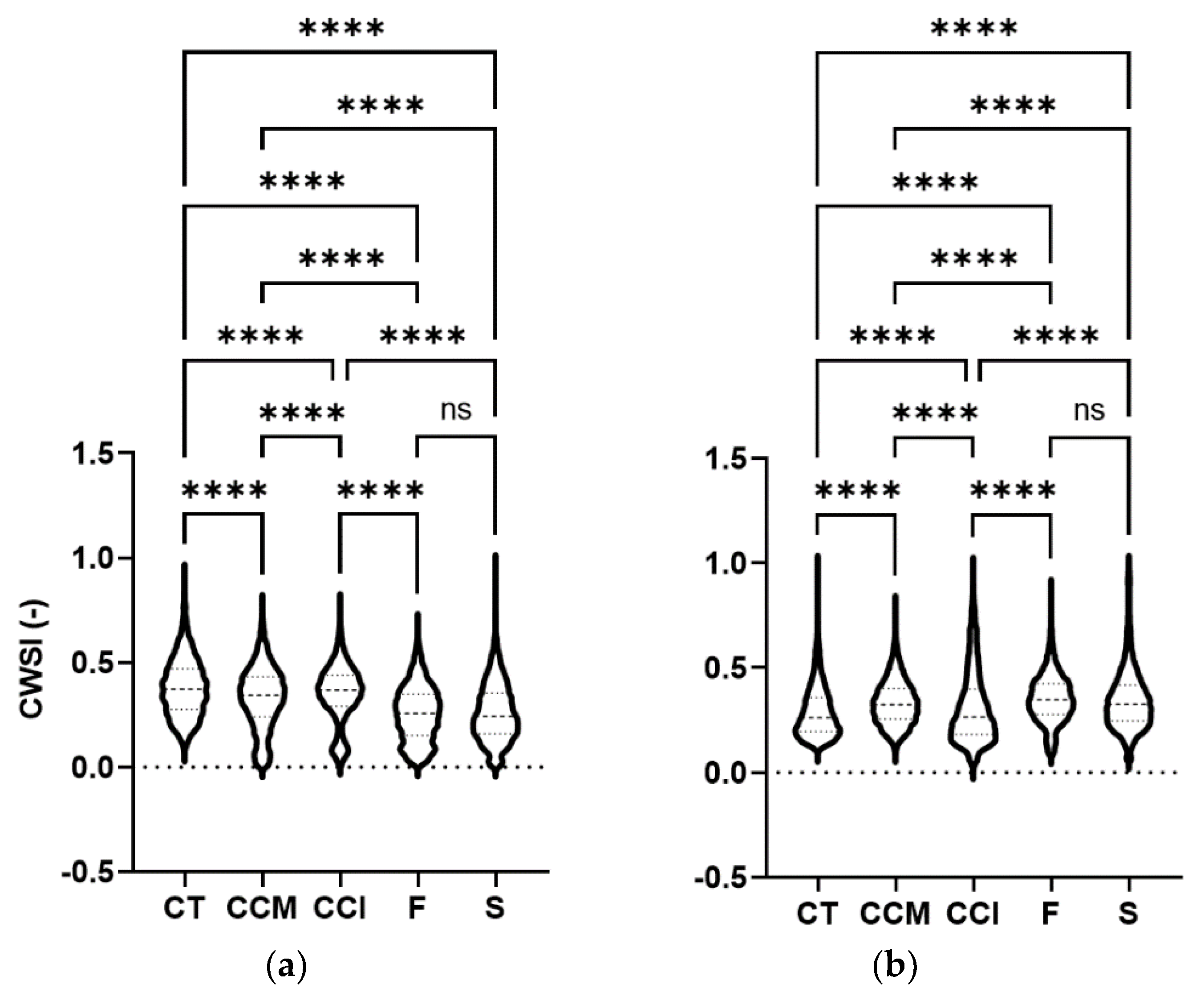
3.4. Mapping CWSI and Discrimination of Treatments

Table 3 shows the Twet and Tdry temperatures for all the treatments extracted from the unimodal histograms by considering the average of the lowest and the highest 0.5% canopy temperatures to compute Twet and Tdry reference, respectively [36].
The CWSI spatial distribution displayed the same pattern as the surface temperature spectral images maps (Figure 11a,b). Therefore, the CWSI maps evidenced a gradient of the stress in SG from the less stressed area in the North-West to the most stressed area in the South-East part of the plot. On the other hand, in MV, the most stressed area was around the center of the field, and the less stressed ones were found at the top and bottom end of the map, confirming what was seen with the map of surface temperature.
The relationship between CWSI vs. MSWP is shown in Figure 12a,b. The size of the bubble is proportional to the slope gradient, whereas the value next to the bubble indicates the NDVI value.
The vineyards of SG experienced no to mild stress levels regarding MSWP, while MV vineyards presented values of mild to high water stress, according to the water stress range proposed by [46].
There is a positive correlation between MSWP and CWSI for both farms, which was significant only in MV (R2 = 0.59). At the same time, this correlation is linked to the NDVI in both farms, which showed lower values of NDVI with higher water stress values. The effect of the slope gradient was correlated in MV, which relationship depicted that as the altitude was lower, the stress values were lower. On the other hand, the crop water status response to the slope gradient was not confirmed in SG, which effect could have been masked by the transversal gradient of the soil chemical-physical properties: combined effect of active limestone and gravel. In addition, we acknowledge that water stress domain of SG was null to mild (e.g., below 8 bar) and narrow, with small variability among the MSWP measurements. Therefore, the crop water status would present a homogeneous condition, which would not be depicted in the correlation between MSWP and CWSI.
Figure 13a,b shows the CWSI multiple comparison among soil management treatments using violin data encoding and the pairwise comparison according to the Tukey’s test. The S and F treatments were not statistically different in both farms, whereas the other paired wise combination of soil management treatments depicted significant statistical differences.
The violin plot analysis showed that on average S and F are the treatments with lower stress values in terms of CWSI for MV. In particular, the violin plot depicts an asymmetric distribution for the S and F compared to the other three soil management treatments. The asymmetric distributions present the median of S and F localized towards the lower values of CWSI.
The lowest stress values evidenced in the S and F treatments in MV could be associated to the beneficial gain due to the cover crop residual fertility effect (e.g., residual N from symbiotic N2–fixation) in F or to the long-lasting presence of spontaneous plant-soil cover in S.
On the other hand, this gain due to the cover crop residual effect could not be perceived in SG, which may be due to the low variability of the MSWP among the treatments and to the disturbance associated to the gravel–active limestone combination covering the difference in terms of crop thermal status.

4. Discussion

The results presented in this study highlight the advantages of using an integrated methodology to discretize among soil management treatments in vineyards from complex territories using GIS tools, aerial thermal and spectral imaging. The methodology suggested presents several advantages compared to traditional techniques, which are time-consuming, discrete and with lower capability to characterize a whole vineyard plot [40].
The outcomes obtained using remotely sensed numerical data have demonstrated that surface temperature and the simplified CWSI, with the support of VIs, would be competent for the discrimination of the most appropriate soil management practices in vineyards.

4.1. Variability within the Vineyard Systems

The vineyards in Chianti terroir are complex agroecological systems much variable in terms of soil texture, topography, and microclimates, which could have an effect on how the soil management techniques influence the crop performance and functional status. In fact, the variability of soil characteristics was one of the main factors explaining the spatial variability of vine biophysical and physiological status (e.g., vigor and water status), which was verified in previous studies on vineyards [4,16,47,48].
The analysis of the particle size composition and chemical components of the soil highlighted, respectively, high content in gravel and active limestone in both farms. The gravel component was the main soil component determining differences on vine performance when was analyzed together with the spatial variability of spectral and thermal indexes. Consequently, our study evidenced a strong influence of the gravel content on the vine vigor. The gravel component is composed of lithoid fragments with low specific surface area, which diminishes the soil water retention properties [49]. Therefore, the lower water retention in the soil during the dry season due to the presence of gravel could lead to a higher incidence of the soil water deficit on the vine growth. In a similar study [10], which was focused on diverse soil management treatments in vineyards, the masking effect of the calcareous content and stony soils did not allow to discriminate the performance among permanent, temporary cover crops and weed management. Consequently, the ranges of active limestone (3.4 ± 4.3 g kg−1) and gravel content (17.8 ±14.9 %), which were lower than the one determined in our study, masked the effects derived from the treatments on the vines’ status [10].

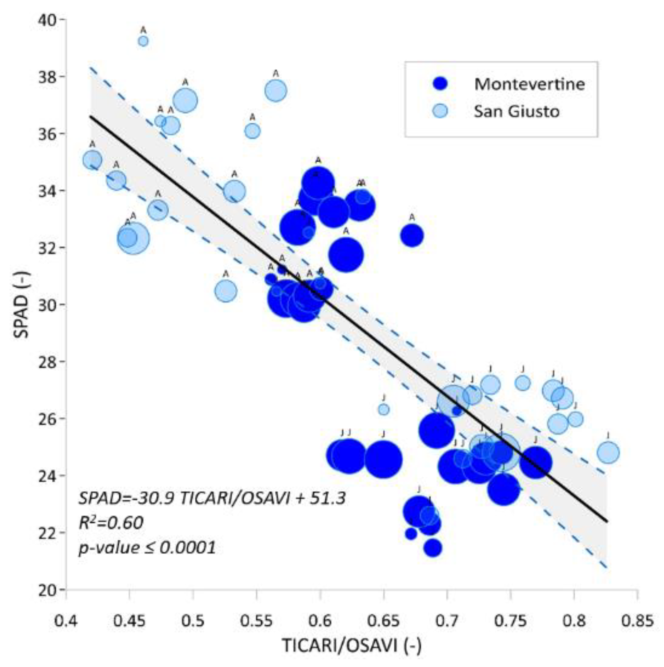
4.2. Spectral Vegetation and Thermal Indexes to Discriminate among Treatments

The NDVI and TCARI/OSAVI indexes served as a supporting tool for the thermal-based indexes. The maps of vine vigor and chlorophyll concentration followed the same spatial patterns as gravel and active limestone concentrations, which confirmed the crop response to these soil components [4,50,51].
Rey-Caramés et al. (2015) [52] has shown an NDVI range (0.57–0.73) similar to ours in vineyards from Navarra (Spain), as well as, [53] with a range of NDVI values (0.765 ± 1.82) within Pinot Noir vineyards fields in Canada. The authors associated the NDVI spatial variability to environmental biophysical constraints, such as low soil water availability, and therefore lower vine size.
The NDVI and the LAI measurements were significantly correlated (R2 = 0.89) at the veraison vine stage in both farms. Therefore, this relationship made possible to consider the NDVI variability as an expression of the crop vigor [54,55,56]. Additionally, the TCARI/OSAVI was linearly correlated to SPAD measurements considering the same time target. Thus, the index is a good indicator of the photosynthetically active part of the vine crop, specifically the leaf chlorophyll a+b content in the plant. The results are consistent with previously published studies on vineyards, which confirmed TCARI/OSAVI as the most consistent indicator of vineyard pigment content [4,30,50,57].
The NDVI statistic indicators individuated which treatment developed more vigorous vine canopies. The frequency distributions of the NDVI were bimodal, representing vine vegetation and soil background due to the different reflectance values of these two features [42]. In both farms, the S treatment presented the highest second mode of the bimodal frequency distribution (e.g., higher NDVI values), which corresponded to the crop vegetation, while the CT depicted the opposite behavior. The first mode of the frequency distribution, thus the soil background effect, was more pronounced in the CT treatment. Hence, the vine growing conditions derived from the S treatment could be more favorable for the vineyard in terms of available soil moisture. In addition, the less vigorous canopies of the CT would present minor water conservation and higher depletion of the available moisture within the vine root zone. This fact could be related to the higher sensible heat in the CT treatment, which leads to higher transpiration of the vine tree and higher soil evaporation, thus causing higher soil water depletion.
Moreover, the crop growth could have been mainly affected by soil water deficit at the veraison stage in August, which was reflected in a lower IR reflectance of chlorophylls that turned into lower plant vigor and thus lower NDVI values [16,18].
Thermal based indices were the core method in this study to assess the physiological condition of the vineyards associated with the application of several soil management treatments. Thermal based indices have been proposed as indicators of plant water stress since the 1960s [19,21,48]. Furthermore, our study goes further and introduced them as a tool to differentiate the best soil management technique in complex territories. To support the validity of the CWSI, a strong linear correlation with MSWP has been found in MV, which was higher than the one in [4] and in accordance with [47,58].
These relationships are confirmed by those reported in annual crops, fruit trees and grapevines, in which CWSI was the indicator that better reflected the crop water status and the root zone moisture content [20,24,39,47,48,58]. In addition, the correlation found between the effect of the slope gradient and the CWSI in MV was in line with previous findings, which confirmed that lower parts of the field slope present higher soil water contents [59].
The correlation between NDVI and CWSI evidenced the chronic or cumulative water stress because is affected by long-term scarce water supply from rainfall. As demonstrated in [58], the authors found a significant inverse correlation between the CWSI and vigor measurements, which evidenced the link between the level of stress of the crop and the vine vigor in semi-arid climates. Hence, CWSI would be a feasible indicator that reflects both immediate and long-term exposure to stress in grapevines.
The surface temperature and CWSI maps displayed similar visual patterns as the ones developed for the spectral vegetation indices, which demonstrated the link between all these variables and the use of VIs as a supporting tool for thermal imaging. Previously, [4] evidenced the relationship among thermal and spectral indices on detecting vine water status and proposed them as a decision support tool.
The frequency distribution of the surface temperatures enabled the more accurate discrimination of the soil management treatments in both farms. Several studies demonstrated the ability of canopy temperature to discriminate among irrigation treatments and thus represent different water status conditions [39,47,58]. As highlighted by the NDVI statistical indicators, the mode that describes the effect of the soil was flattened and difficult to discriminate in the S treatment, followed by the F treatment. This fact suggests that the vine vigor was maximum in the S and F treatments, which canopies covered wider areas diminishing the warmer soil temperatures. There would be an effect of the S vegetation and F cover crop on the vine water status, since these kinds of combinations keep more water in the soil available to the vine, as has been shown in several studies on cover cropped vineyards [7,60]. The vegetation of the cover crop could increase soil water availability by enhancing water infiltration and conservation, and then lower the average canopy surface temperature, which is correlated to a higher canopy transpiration process. This fact was pointed out in diverse studies in which soil management strategies induced changes in the vine canopy microclimate [18,45].
Regarding the S treatment, our results are in agreement with previous studies that reported spontaneous native vegetation as the most adequate cover to increase soil water availability in Mediterranean vineyards [61,62].
According to these outcomes, the agroecosystem under study can be seen as composed by three buckets, which are formed by the vine roots, the cover crop roots and a bucket where there is neither one nor the other [63]. The cover crop bucket played a conservative role, which means that it kept more water in the soil and built a reservoir that increased water availability to the vine row, as observed also in other studies [12,62]. Consequently, the cover crop/grassing bucket increased the soil water availability for the vine row, while the same bucket modified the microclimate conditions of the vine row by lowering its sensible heat [64,65].
From an agroecological point of view, it can be hypothesized that the S treatment has shown lower competition for soil resources. Thus, the S treatment showed higher conservation capacity of water and soil nutrients from the early vegetative growth stage in spring to post-harvest in autumn. On the other hand, the positive effect of the F treatment on the thermal status of the vine may have been due to an improvement of the soil nutritional conditions, e.g., through higher N availability in the vine root zone as a result of N2–fixation of pigeon bean.
On the other hand, the CT treatment was frequently tilled and did not have a soil cover and the vine row thermal status might have been affected by the higher contribute of sensible heat. This is confirmed by a more marked soil mode and at the same time the vegetation mode situated towards higher temperature values. Reference [65] evidenced higher soil temperatures on tillage when compared to cover cropped soil, especially during the warmer months.

5. Conclusions

This study used a simplified and non-invasive methodology to discriminate how different soil management practices affect the water status in rainfed vineyards. High-resolution spectral imagery acquired from UAV and GIS tools allowed to investigate the whole spatial variability of the vineyard water status within the field and distinguish the effect of the soil chemical and physical properties.
This approach was able to discriminate the spontaneous grass vegetation (S) and pigeon bean (F) cover crop as the optimal management treatments for both experimental farms. The results showed, on average, that surface temperature of the vine’s canopy was lower for the S and F treatments, and the same results were found in terms of CWSI and vegetation spectral indexes. In addition, it was found that gravel and active limestone content determined the spatial patterns of vine biophysical and physiological characteristics. Hence, soil properties could influence the efficiency of the soil practices implemented.
The combined approach would be further applied to assess the best combination of cover crop species/mixtures and management techniques (e.g., mowing, green manure, mulching) in diverse pedoclimatic conditions, which would reflect the spatial soil variability present in the vineyards from the Mediterranean regions. Specifically, Chianti’s winegrowers could use the integrated methodology to adopt the best soil management in their specific territory, due to the complexity of Chianti terroir.
The territory understudy is suffering from acute drought periods that are affecting vineyards performance. Thus, further research would be focused on combining soil management by applying supplemental irrigation while monitoring productive and quality parameters, which could help wine growers alleviate the water stress periods.

Author Contributions

À.P.-S.: conceptualization, methodology, investigation, data curation, writing—original draft. D.A.: investigation, validation, writing—review and editing. D.W.R.: investigation, validation, writing—review and editing. G.R.: conceptualization, methodology, data curation, writing—review and editing. All authors have read and agreed to the published version of the manuscript.

Funding

The research was carried out in the frame of “Progetto OP-Illuminati Frutta-Rallo” (University of Pisa, MIPAF-Regione Toscana) and “ATMOSMART-dimostratore tecnologico” (University of Pisa). The field experiments are partly funded by the EU-H2020 Project “IWMPRAISE” (GA nr. 727321).

Acknowledgments

Montevertine and San Giusto a Rentennano for offering their plots and availability to carry out the experiments; SPEVIS s.r.l. (Stazione Sperimentale di Viticoltura Sostenibile, Panzano in Chianti, Florence, Italy), Ing. Simone Katsiotis (DroneBee|Agricoltura Intelligente) and Andrea Sbrana to support the research.

Conflicts of Interest

The authors declare no conflict of interest.

References

  1. Van Leeuwen, C.; Darriet, P. The Impact of Climate Change on Viticulture and Wine Quality. J. Wine Econ. 2016, 11, 150–167. [Google Scholar] [CrossRef] [Green Version]
  2. Anderson, K.; Nelgen, S. Global Wine Markets, 1961 to 2009: A Statistical Compendium; University of Adelaide Press: Adelaide, Australia, 2011. [Google Scholar]
  3. Medrano, H.; Tomás, M.; Martorell, S.; Escalona, J.-M.; Pou, A.; Fuentes, S.; Flexas, J.; Bota, J. Improving water use efficiency of vineyards in semi-arid regions. A review. Agron. Sustain. Dev. 2015, 35, 499–517. [Google Scholar] [CrossRef] [Green Version]
  4. Baluja, J.; Diago, M.P.; Balda, P.; Zorer, R.; Meggio, F.; Morales, F.; Tardaguila, J. Assessment of Vineyard Water Status Variability by Thermal and Multispectral Imagery Using an Unmanned Aerial Vehicle (UAV). Irrig. Sci. 2012, 30, 511–522. [Google Scholar] [CrossRef]
  5. Novara, A.; Cerdà, A.; Gristina, L. Sustainable vineyard floor management: An equilibrium between water consumption and soil conservation. Curr. Opin. Environ. Sci. Health 2018, 5, 33–37. [Google Scholar] [CrossRef]
  6. Morlat, R.; Jacquet, A. Grapevine root system and soil characteristics in a vineyard maintained long-term with or without interrow sward. Am. J. Enol. Vitic. 2003, 54, 1–7. [Google Scholar]
  7. Tomaz, A.; Pacheco, C.A.; Coleto Martinez, J.M. Influence of cover cropping on water uptake dynamics in an irrigated Mediterranean vineyard. Irrig. Drain. 2017, 66, 387–395. [Google Scholar] [CrossRef]
  8. Garcia, L.; Celette, F.; Gary, C.; Ripoche, A.; Valdés-gómez, H. Agriculture, Ecosystems and Environment Management of service crops for the provision of ecosystem services in vineyards: A review. Agric., Ecosyst. Environ. 2018, 251, 158–170. [Google Scholar] [CrossRef] [Green Version]
  9. Mercenaro, L.; Nieddu, G.; Pulina, P.; Porqueddu, C. Agriculture, Ecosystems and Environment Sustainable management of an intercropped Mediterranean vineyard. Agric. Ecosyst. Environ. 2014, 192, 95–104. [Google Scholar] [CrossRef]
  10. Salomé, C.; Coll, P.; Lardo, E.; Metay, A.; Villenave, C.; Marsden, C.; Blanchart, E.; Hinsinger, P.; Le Cadre, E. The soil quality concept as a framework to assess management practices in vulnerable agroecosystems: A case study in Mediterranean vineyards. Ecol. Indic. 2016, 61, 456–465. [Google Scholar] [CrossRef]
  11. Baiamonte, G.; Minacapilli, M.; Novara, A.; Gristina, L. Time scale effects and interactions of rainfall erosivity and cover management factors on vineyard soil loss erosion in the semi-arid area of southern Sicily. Water 2019, 11, 978. [Google Scholar] [CrossRef] [Green Version]
  12. Ogilvie, C.M.; Deen, W.; Martin, R.C. Service crop management to maximize crop water supply and improve agroecosystem resilience: A review. J. Soil Water Conserv. 2019, 74, 389–404. [Google Scholar] [CrossRef]
  13. Cerdà, A.; Rodrigo-Comino, J.; Giménez-Morera, A.; Keesstra, S.D. Hydrological and erosional impact and farmer’s perception on catch crops and weeds in citrus organic farming in Canyoles river watershed, Eastern Spain. Agric. Ecosyst. Environ. 2018, 258, 49–58. [Google Scholar] [CrossRef]
  14. Yang, Y.T. Evapotranspiration over Heterogeneous Vegetated Surfaces. Ph.D. Thesis, Tsinghua University, Beijing, China, 2015. [Google Scholar]
  15. Costantini, E.A.C.; Barbetti, R. Environmental and visual impact analysis of viticulture and olive tree cultivation in the province of Siena (Italy). Eur. J. Agron. 2008, 28, 412–426. [Google Scholar] [CrossRef]
  16. Acevedo-Opazo, C.; Tisseyre, B.; Ojeda, H.; Ortega-Farias, S.; Guillaume, S. Is it possible to assess the spatial variability of vine water status? OENO ONE 2008, 42, 203–219. [Google Scholar] [CrossRef]
  17. Bellvert, J.; Zarco-Tejada, P.J.; Girona, J.; Fereres, E. Mapping Crop Water Stress Index in a ‘Pinot-Noir’ Vineyard: Comparing Ground Measurements with Thermal Remote Sensing Imagery from an Unmanned Aerial Vehicle. Precis. Agric. 2014, 15, 361–376. [Google Scholar] [CrossRef]
  18. Gago, J.; Douthe, C.; Coopman, R.E.; Gallego, P.P.; Ribas-Carbo, M.; Flexas, J.; Escalona, J.; Medrano, H. UAVs challenge to assess water stress for sustainable agriculture. Agric. Water Manag. 2015, 153, 9–19. [Google Scholar] [CrossRef]
  19. Methodologies and Results in Grapevine Research; Delrot, S.; Medrano-Gil, H.; Or, E.; Bavaresco, L.; Grando, S. (Eds.) Springer Science+Business Media, B.V.: Dordrecht, The Netherlands, 2010. [Google Scholar]
  20. Gutiérrez, S.; Diago, M.P.; Fernández-Novales, J.; Tardaguila, J. Vineyard water status assessment using on-the-go thermal imaging and machine learning. PLoS ONE 2018, 13, e0192037. [Google Scholar] [CrossRef] [PubMed]
  21. Tanner, C.B. Plant temperatures. Agron. J. 1963, 55, 210–211. [Google Scholar] [CrossRef]
  22. Jackson, R.; Idso, S.; Reginato, R.; Pinter, P.J. Canopy temperature as a crop water stress indicator. Water Resour. Res. 1981, 17, 1133–1138. [Google Scholar] [CrossRef]
  23. Idso, S.B.; Jackson, R.D.; Pinter, P.J.; Reginato, R.J.; Hatfield, J.L. Normalizing the stress-degree day parameter for environmental variability. Agric. Meteorol. 1981, 24, 45–55. [Google Scholar] [CrossRef]
  24. Park, S.; Nolan, A.P.; Ryu, D.; Chung, H. Estimation of crop water stress in a nectarine orchard using high-resolution imagery from unmanned aerial vehicle (UAV). In Proceedings of the MODSIM2015, 21st International Congress on Modelling and Simulation, Modelling and Simulation Society of Australia and New Zealand, Gold Coast, Australia, 29 November–4 December 2015; pp. 1413–1419. [Google Scholar]
  25. Jiménez-Berni, J.A.; Zarco-Tejada, P.J.; Sepulcre-Cantó, G.; Fereres, E.; Villalobos, F. Mapping canopy conductance and CWSI in olive orchards using high resolution thermal remote sensing imagery. Remote Sens. Environ. 2009, 113, 2380–2388. [Google Scholar] [CrossRef]
  26. Retzlaff, R.; Molitor, D.; Behr, M.; Bossung, C.; Rock, G.; Hoffmann, L.; Evers, D.; Udelhoven, T. UAS-based multi-angular remote sensing of the effects of soil management strategies on grapevine. J. Int. Sci. Vigne Vin 2015, 49, 85–102. [Google Scholar] [CrossRef] [Green Version]
  27. Autovino, D.; Rallo, G.; Provenzano, G. Predicting soil and plant water status dynamic in olive orchards under different irrigation systems with Hydrus-2D: Model performance and scenario analysis. Agr. Water Manag. 2018, 203, 225–235. [Google Scholar] [CrossRef]
  28. Haboudane, D.; Miller, J.R.; Tremblay, N.; Zarco-Tejada, P.J.; Dextraze, L. Integrated narrow-band vegetation indices for prediction of crop chlorophyll content for application to precision agriculture. Remote Sens. Environ. 2002, 81, 416–426. [Google Scholar] [CrossRef]
  29. Martín, P.; Zarco-Tejada, P.J.; González, M.R.; Berjón, A. Using hyperspectral remote sensing to map grape quality in “Tempranillo” vineyards affected by iron deficiency chlorosis. VITIS J. Grapevine Res. 2015, 46, 7. [Google Scholar]
  30. Zarco-tejada, P.J.; Berjón, A.; López-Lozano, R.; Miller, J.; Martín, P.; Cachorro, V.; González, M.; de Frutos, A. Assessing vineyard condition with hyperspectral indices: Leaf and canopy reflectance simulation in a row-structured discontinuous canopy. Remote. Sens. Environ. 2005, 99, 271–287. [Google Scholar] [CrossRef]
  31. Zarco-Tejada, P.J.; Guillén-Climent, M.L.; Hernández-Clemente, R.; Catalina, A.; González, M.R.; Martín, P. Estimating Leaf Carotenoid Content in Vineyards Using High Resolution Hyperspectral Imagery Acquired from an Unmanned Aerial Vehicle (UAV). Agric. For. Meteorol. 2013, 171–172, 281–294. [Google Scholar] [CrossRef] [Green Version]
  32. Ditzler, C.; Scheffe, K.; Monger, H.C.; Soil Science Division Staff. Soil Survey Manual. USDA Handbook 18; Government Printing Office: Washington, DC, USA, 2017.
  33. Drouineau, G. Rapid determination of the active limestone soil. Reportation new data on the nature of the limestone fractions. Ann. Agron. 1942, 12, 441–450. [Google Scholar]
  34. QGIS Geographic Information System. Open Source Geospatial Foundation Project. 2020. Available online: http://qgis.org (accessed on 1 January 2021).
  35. Welles, J.M.; Norman, J.M. Instrument for indirect measurement of canopy architecture. Agron. J. 1991, 83, 818–825. [Google Scholar]
  36. Turner, N.C. Techniques and experimental approaches for the measurement of plant water status. Plant Soil 1981, 58, 339–366. [Google Scholar] [CrossRef]
  37. Rouse, J.W.; Haas, R.H.; Schell, J.A.; Deering, D.W. Monitoring vegetation systems in the Great Plains with ERTS. NASA Spec. Publ. 1974, 351, 309. [Google Scholar]
  38. Rondeaux, G.; Steven, M.; Baret, F. Optimization of soil-adjusted vegetation indices. Remote Sens. Environ. 1996, 55, 95–107. [Google Scholar] [CrossRef]
  39. Bian, J.; Zhang, Z.; Chen, J.; Chen, H.; Cui, C.; Li, X.; Chen, S.; Fu, Q. Simplified evaluation of cotton water stress using high resolution unmanned aerial vehicle thermal imagery. Remote Sens. 2019, 11, 267. [Google Scholar] [CrossRef] [Green Version]
  40. González-Dugo, V.; Zarco-Tejada, P.; Nicolas, E.; Nortes, P.A.; Alarcón, J.J.; Intrigliolo, D.S.; Fereres, E. Using high resolution UAV thermal imagery to assess the variability in the water status of five fruit tree species within a commercial orchard. Precis. Agric. 2013, 14, 660–678. [Google Scholar] [CrossRef]
  41. Duarte, L.; Silva, P.; Teodoro, A.C. Development of a QGIS plugin to obtain parameters and elements of plantation trees and vineyards with aerial photographs. Int. J. Geo-Inf. 2018, 7, 14–19. [Google Scholar] [CrossRef] [Green Version]
  42. Hall, A.; Louis, J.; Lamb, D. Characterising and mapping vineyard canopy using high-spatial-resolution aerial multispectral images. Comput. Geosci. 2003, 29, 813–822. [Google Scholar] [CrossRef]
  43. Sepulcre-cantó, G.; Zarco-tejada, P.J.; Jiménez-Muñoz, J.; Sobrino, J.A.; de Miguel, E.; Villalobos, F.J. Detection of water stress in an olive orchard with thermal remote sensing imagery. Agric. For. Meteorol. 2006, 136, 31–44. [Google Scholar] [CrossRef]
  44. Gerhards, M.; Schlerf, M.; Id, U.R.; Udelhoven, T.; Juszczak, R.; Alberti, G.; Id, F.M.; Inoue, Y. Analysis of Airborne Optical and Thermal Imagery for Detection of Water Stress Symptoms. Remote. Sens. 2018, 10, 1139. [Google Scholar] [CrossRef] [Green Version]
  45. O’Brien, P.L.; Daigh, A.L.M. Tillage practices alter the surface energy balance—A review. Soil Tillage Res. 2019, 195, 104354. [Google Scholar] [CrossRef]
  46. Poblete-Echeverría, C.; Espinace, D.; Sepúlveda-Reyes, D.; Zúñiga, M.; Sanchez, M. Analysis of crop water stress index (CWSI) for estimating stem water potential in grapevines: Comparison between natural reference and baseline approaches. Acta Hortic. 2017, 1150, 189–194. [Google Scholar] [CrossRef]
  47. Bellvert, J.; Marsal, J.; Girona, J.; Gonzalez-dugo, V.; Fereres, E.; Ustin, S.L.; Zarco-tejada, P.J. Airborne Thermal Imagery to Detect the Seasonal Evolution of Crop Water Status in Peach, Nectarine and Saturn Peach Orchards. Remote Sens. 2016, 8, 39. [Google Scholar] [CrossRef] [Green Version]
  48. Santesteban, L.G.; Di Gennaro, S.F.; Herrero-langreo, A.; Miranda, C.; Royo, J.B.; Matese, A. High-resolution UAV-based thermal imaging to estimate the instantaneous and seasonal variability of plant water status within a vineyard. Agric. Water Manag. 2017, 183, 49–59. [Google Scholar] [CrossRef]
  49. Murray, E.J.; Sivakumar, V. Unsaturated Soils: A Fundamental Interpretation of Soil Behaviour; Wiley: New York, NY, USA, 2010. [Google Scholar]
  50. Haboudane, D.; Tremblay, N.; Miller, J.R.; Vigneault, P. Using Spectral Indices Derived From Hyperspectral Data. Geosci. Remote. Sens. IEEE 2008, 46, 423–437. [Google Scholar] [CrossRef]
  51. Gil-Pérez, B.; Zarco-Tejada, P.J.; Correa-Guimaraes, A.; Relea-Gangas, E.; Navas-Gracia, L.M.; Hernández-Navarro, S.; Sanz-Requena, J.F.; Berjón, A.; Martín-Gil, J. Remote sensing detection of nutrient uptake in vineyards using narrow-band hyperspectral imagery. Vitis J. Grapevine Res. 2010, 49, 167–173. [Google Scholar]
  52. Rey-Caramés, C.; Diago, M.; Martín, M.; Lobo, A.; Tardaguila, J. Using RPAS Multi-Spectral Imagery to Characterise Vigour, Leaf Development, Yield Components and Berry Composition Variability within a Vineyard. Remote Sens. 2015, 7, 14458–14481. [Google Scholar] [CrossRef] [Green Version]
  53. Reynolds, A.G.; Brown, R.; Kotsaki, E.; Lee, H.-S. Utilization of proximal sensing technology (greenseeker) to map variability in ontario vineyards. In Proceedings of the 19th International Symposium GiESCO, Gruissan, France, 31 May–5 June 2015; pp. 593–597. [Google Scholar]
  54. Montero, F.J.; Meliá, J.; Brasa, A.; Segarra, D.; Cuesta, A.; Lanjeri, S. Assessment of vine development according to available water resources by using remote sensing in La Mancha, Spain. Agric. Water Manag. 1999, 40, 363–375. [Google Scholar] [CrossRef]
  55. Johnson, L.F. Temporal stability of an NDVI-LAI relationship in a Napa Valley vineyard. Aust. J. Grape Wine Res. 2003, 9, 96–101. [Google Scholar] [CrossRef]
  56. Caruso, G.; Zarco-Tejada, P.J.; González-Dugo, V.; Moriondo, M.; Tozzini, L.; Palai, G.; Rallo, G.; Hornero, A.; Primicerio, J.; Gucci, R. High-resolution imagery acquired from an unmanned platform to estimate biophysical and geometrical parameters of olive trees under different irrigation regimes. PLoS ONE 2019, 14, e0210804. [Google Scholar] [CrossRef] [PubMed] [Green Version]
  57. Soubry, I.; Patias, P.; Tsioukas, V. Monitoring Vineyards with UAV and Multi-sensors for the assessment of Water Stress and Grape Maturity. J. Unmanned Veh. Syst. 2017, 5, 37–50. [Google Scholar] [CrossRef] [Green Version]
  58. Fuentes, S.; De Bei, R.; Pech, J.; Tyerman, S. Computational water stress indices obtained from thermal image analysis of grapevine canopies. Irrig. Sci. 2012, 30, 523–536. [Google Scholar] [CrossRef]
  59. Basile, A.; Albrizio, R.; Autovino, D.; Bonfante, A.; De Mascellis, R.; Terribile, F.; Giorio, P. A modelling approach to discriminate contributions of soil hydrological properties and slope gradient to water stress in Mediterranean vineyards. Agric. Water Manag. 2020, 241, 106338. [Google Scholar] [CrossRef]
  60. Steenwerth, K.; Belina, K.M. Cover crops enhance soil organic matter, carbon dynamics and microbiological function in a vineyard agroecosystem. Appl. Soil Ecol. 2008, 40, 359–369. [Google Scholar] [CrossRef]
  61. Monteiro, A.; Lopes, C.M. Influence of cover crop on water use and performance of vineyard in Mediterranean Portugal. Agric. Ecosyst. Environ. 2007, 121, 336–342. [Google Scholar] [CrossRef]
  62. Trigo-Córdoba, E.; Bouzas-Cid, Y.; Orriols-Fernández, I.; Mirás-Avalos, J.M. Effects of deficit irrigation on the performance of grapevine (Vitis vinifera L.) cv. “Godello” and “Treixadura” in Ribeiro, NW Spain. Agric. Water Manag. 2015, 161, 20–30. [Google Scholar] [CrossRef]
  63. Vismara, R. Ecologia Applicata. 1992. Available online: https://www.libreriauniversitaria.it/ecologia-applicata-vismara-renato-hoepli/libro/9788820315696 (accessed on 16 February 2021).
  64. Nachtergaele, J.; Poesen, J.; van Wesemael, B. Gravel mulching in vineyards of southern Switzerland. Soil Tillage Res. 1998, 46, 51–59. [Google Scholar] [CrossRef]
  65. Ruiz-colmenero, M.; Bienes, R.; Marques, M.J. Soil and water conservation dilemmas associated with the use of green cover in steep vineyards. Soil Tillage Res. 2011, 117, 211–223. [Google Scholar] [CrossRef]
Figure 1. Experimental fields and their set-up for Montevertine (a) and San Giusto a Rentennano farm (b).
Remotesensing 13 00716 g001
Figure 2. Maps of active limestone and gravel content of MV and SG experimental fields.
Remotesensing 13 00716 g002
Figure 3. Correlation between normalized difference vegetation index (NDVI) and leaf area Index (LAI) for the two farms investigated. The error bars indicate the standard deviation of the measurements collected on each pair of transects.
Remotesensing 13 00716 g003
Figure 4. NDVI maps of June and August 2018 for MV and SG.
Remotesensing 13 00716 g004
Figure 5. Distribution frequency of the NDVI pixels and boxplots obtained for the entire vine row treatment and for the three subplots (top; middle; bottom) localized along the slope gradient.
Remotesensing 13 00716 g005
Figure 6. Distribution frequency of the NDVI pixels and boxplots obtained for the entire vine row treatment and for the three subplots (top; middle; bottom) localized along the slope gradient.
Remotesensing 13 00716 g006
Figure 7. TCARI/OSAVI maps of June and August 2018 for MV (a,b) and SG (c,d).
Remotesensing 13 00716 g007
Figure 8. Correlation between TCARI/OSAVI and SPAD acquired on 16 June (J) and 03 August (A). The size of the bubble is proportional to the soil gravel content.
Remotesensing 13 00716 g008
Figure 9. Surface temperature image referred to the entire experimental plots in (a) MV and (b) SG.
Remotesensing 13 00716 g009
Figure 10. Distributions frequency and boxplots of the surface temperature pixels obtained for the entire treatment row and for the three subplots (top; middle; bottom).
Remotesensing 13 00716 g010
Figure 11. Maps of CWSI computed for (a) Montevertine and (b) San Giusto a Rentennano.
Remotesensing 13 00716 g011
Figure 12. Relationship between CWSI vs. MSWP for Montevertine (a) and San Giusto a Rentennano (b). The size of the bubble is proportional to the slope gradient, whereas the number next to the bubble indicates the NDVI value.
Remotesensing 13 00716 g012
Figure 13. Violin data encoding and pairwise comparison of CWSI values computed for the five soil management treatments for Montevertine (a) and San Giusto a Rentennano (b). The asterisks indicate statistical significance (p-value ≤ 0.0001)
Remotesensing 13 00716 g013
Table 1. Description of the experimental treatments.
TreatmentTillage Applied Under TrellisTillage Applied in the Inter-RowCover Crop SpeciesCover Crop Management
Conventional tillage (CT)In-row ventral plowThree-shank grubber at 15 cm depth (autumn, spring, summer)Spontaneous vegetationSpontaneous vegetation incorporated with grubber
Barley-clover dead mulch (CCM)In-row ventral plowThree-shank grubber at 15 cm depth only before cover crop sowing (autumn)Hordeum vulgare L. (85 kg ha−1): Trifolium squarrosum L. (25 kg ha−1)Mowed in late spring and retained as dead mulch
Barley-clover green manure (CCI)In-row ventral plowThree-shank grubber at 15 cm depth only before cover crop sowing (autumn)Hordeum vulgare L. (85 kg ha−1): Trifolium squarrosum L. (25 kg ha−1)Soil incorporated in late spring
Pigeon bean green manure (F)In-row ventral plowThree-shank grubber at 15 cm depth only before cover crop sowing (autumn)Vicia faba L. var. minor Beck (90 kg ha−1)Soil incorporated in late spring
Spontaneous vegetation (S)In-row ventral plowNoneSpontaneous vegetationMowed in late spring
Table 2. Average values (μ) and standard deviation (σ) of the particles size composition (percentage of clay, silt and sand), gravel and percentage of active limestone of Azienda Agricola Montevertine (MV) and Fattoria San Giusto a Rentennano (SG).
FarmClay (%)Silt (%)Sand (%)Gravel (g kg−1)Active Limestone (%)
μσμσμσμσμσ
Montevertine0.280.040.490.050.230.05218.5329.764.530.96
San Giusto0.250.030.430.080.320.05116.2325.426.864.83
Table 3. Twet and Tdry temperatures (°C) of the two farms divided by treatment.
FarmTemperatureCTCCMCCI FS
MontevertineTwet32.5033.0029.0030.1331.63
Tdry44.2545.8844.7544.3843.75
San Giusto a RentennanoTwet30.5028.2527.0026.8828.25
Tdry44.6344.2544.3843.2544.25
Publisher’s Note: MDPI stays neutral with regard to jurisdictional claims in published maps and institutional affiliations.

