
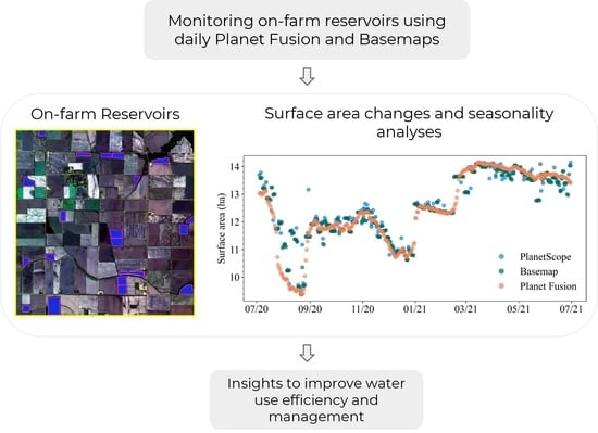
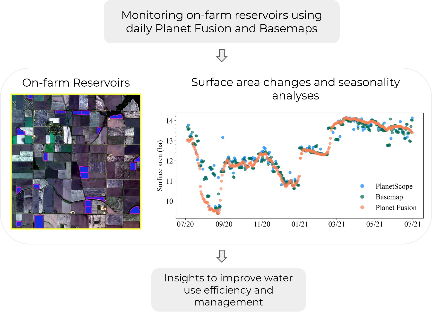
Monitoring Small Water Bodies Using High Spatial and Temporal Resolution Analysis Ready Datasets

 , ,
, ,
Abstract
:
1. Introduction
2. Methods
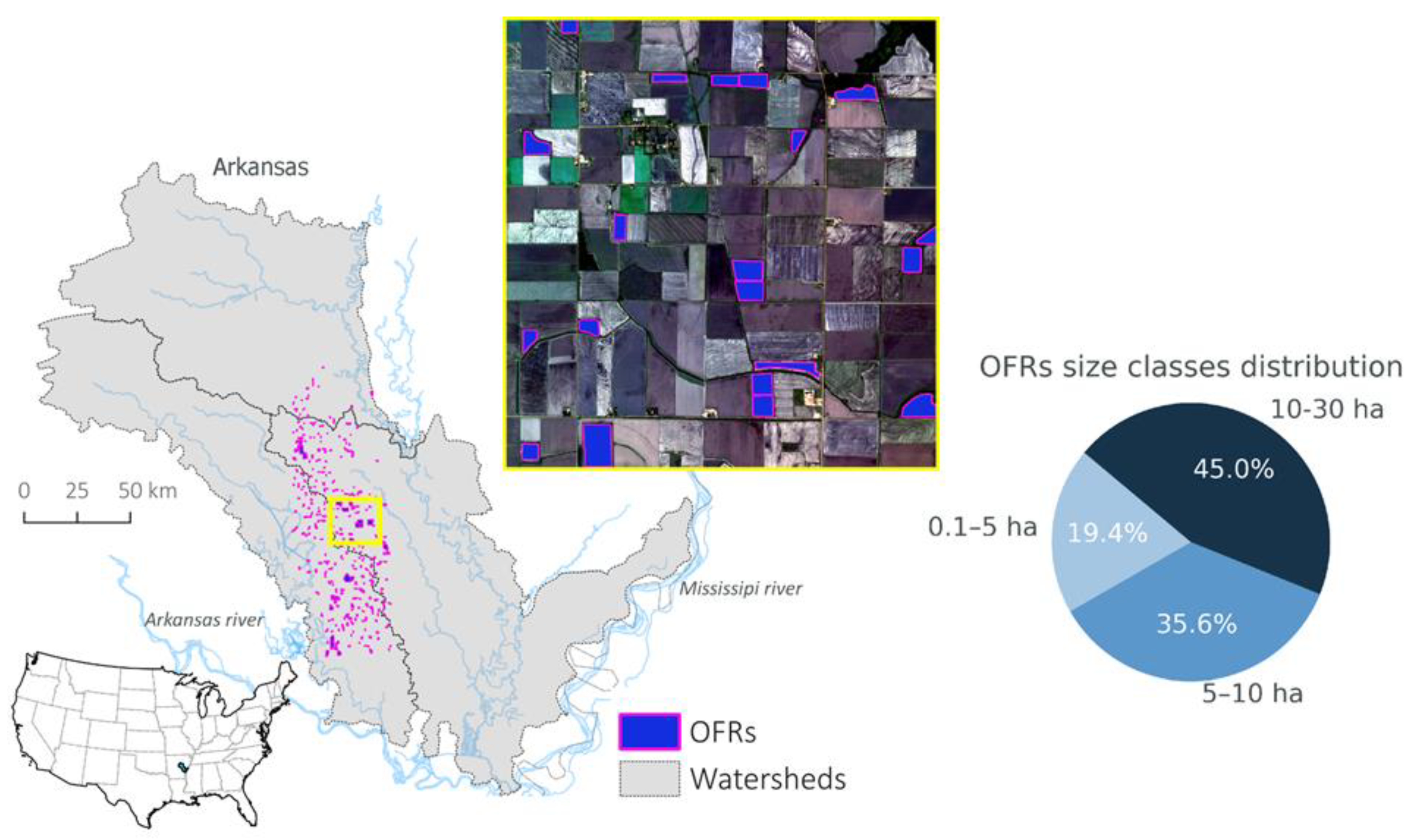
2.1. Study Region
2.2. Satellite Imagery Datasets
2.2.1. PlanetScope CubeSat Surface-Reflectance Ortho Tiles
2.2.2. Normalized Surface-Reflectance Basemap
2.2.3. Planet Fusion Surface Reflectance
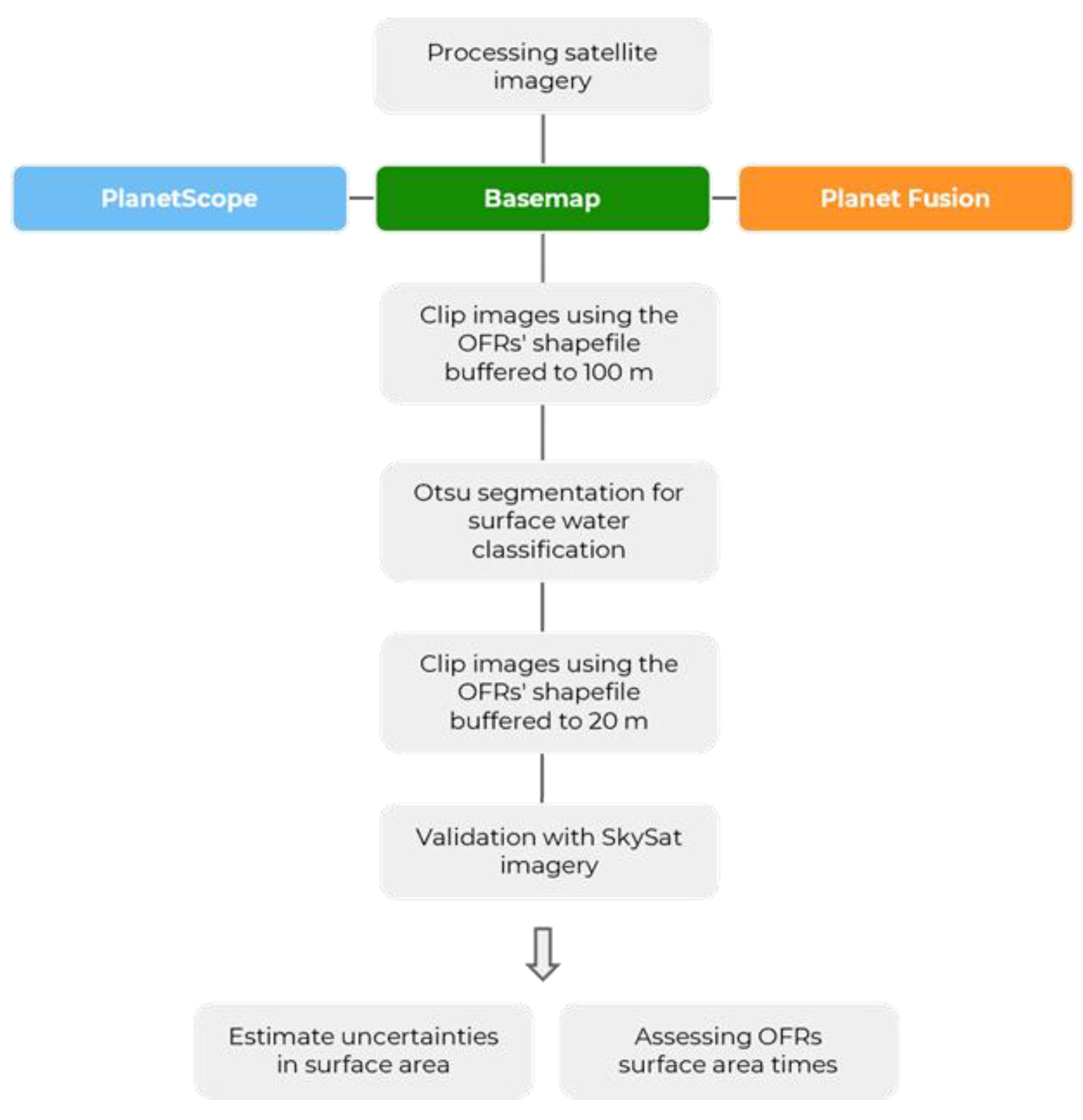
2.3. Data Analysis
2.4. Validation Scheme
3. Results
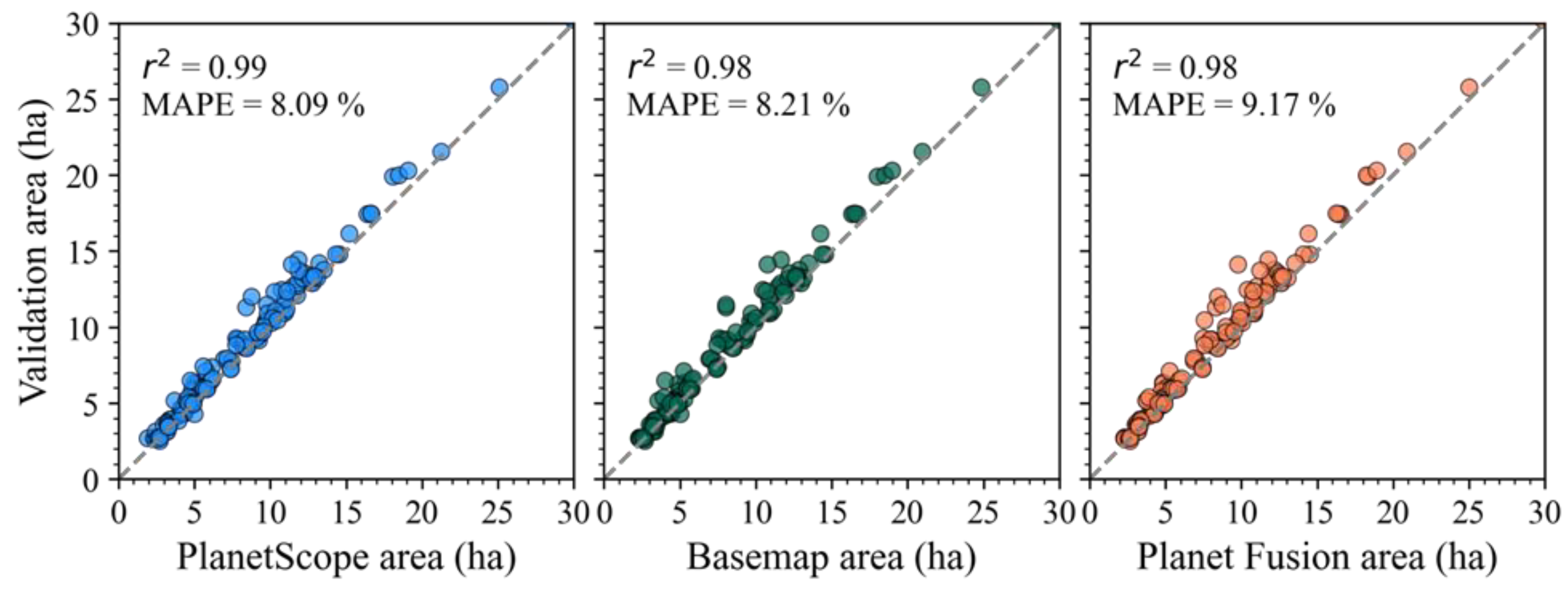
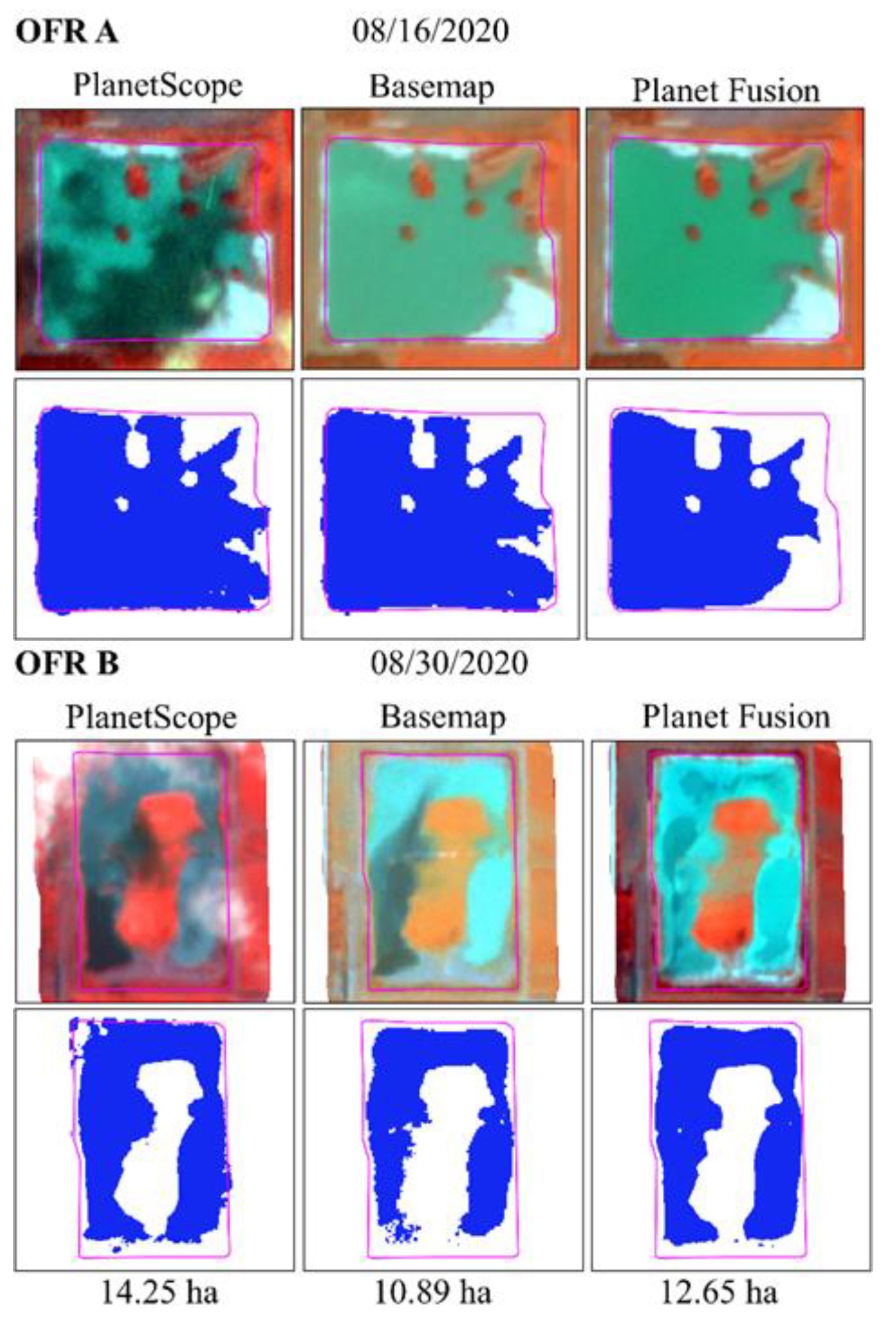
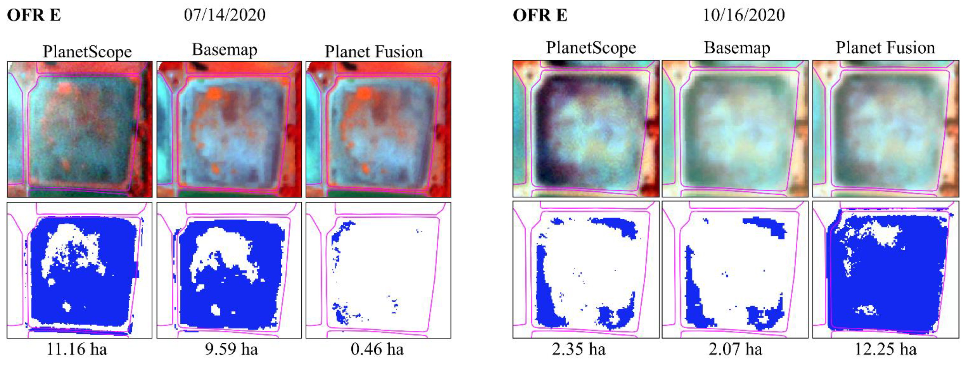
3.1. Surface Water Area Validation Using SkySat Imagery
3.2. Number of Surface Area Observations per Dataset
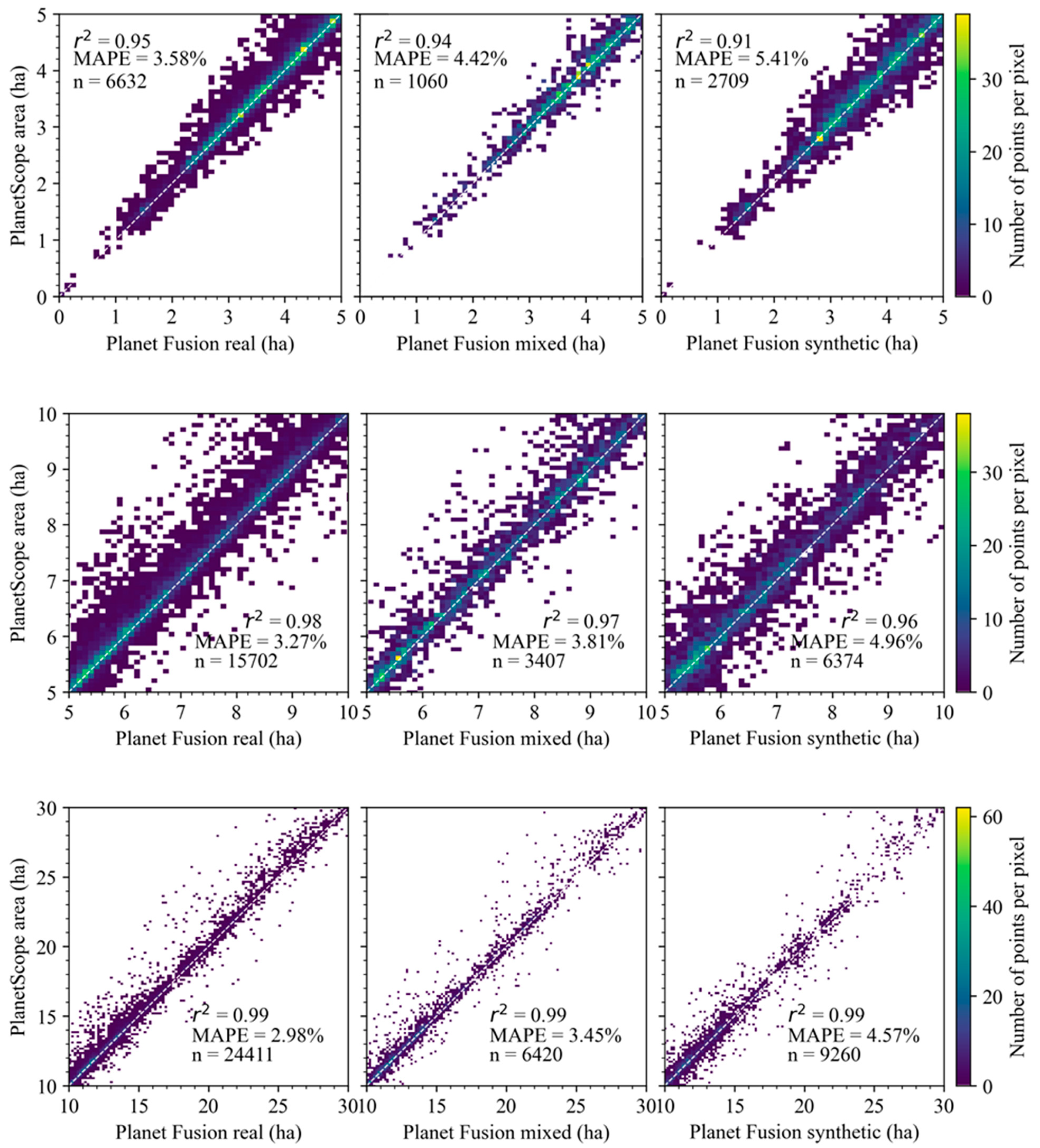
3.3. Planet Fusion Comparison with PlanetScope
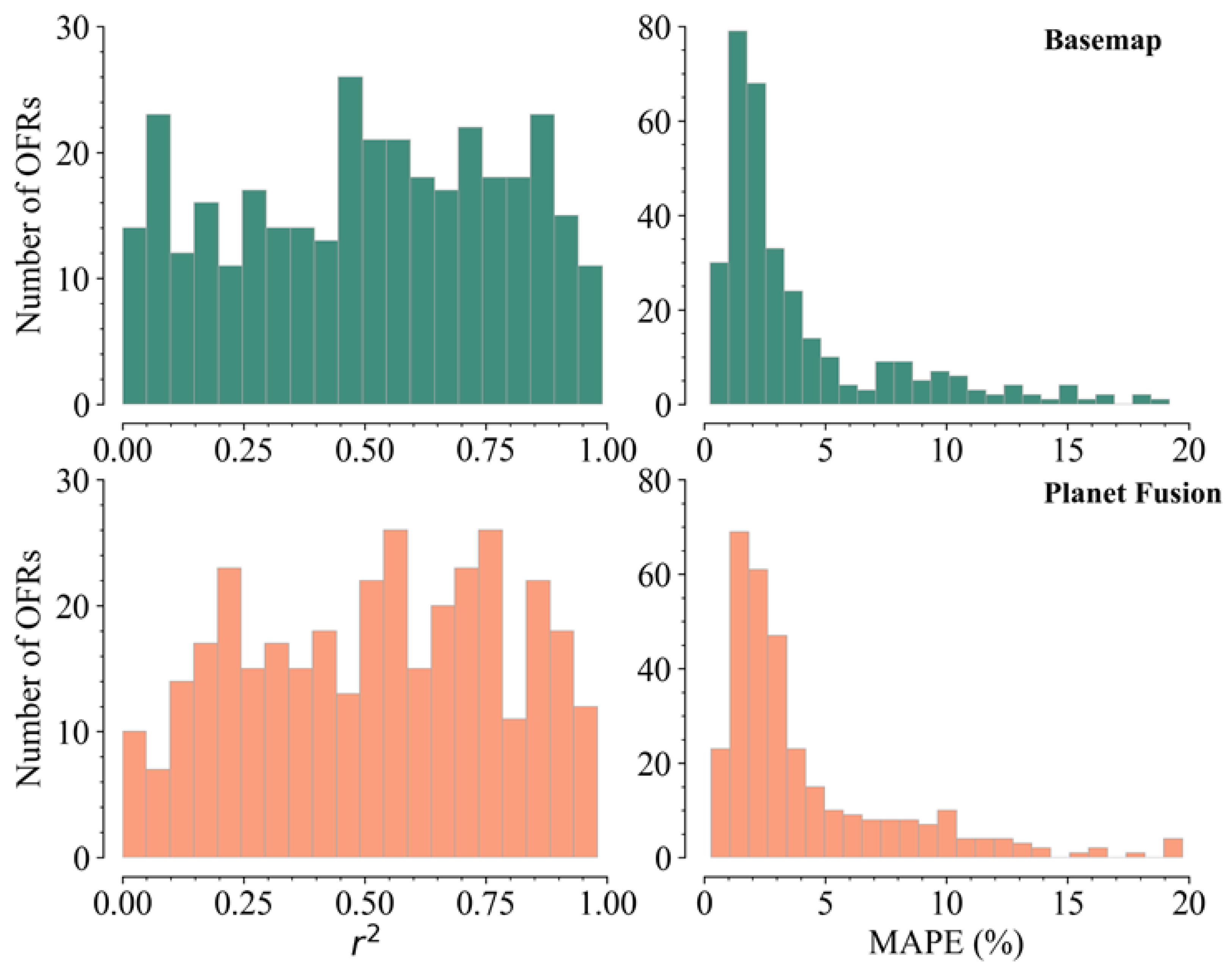
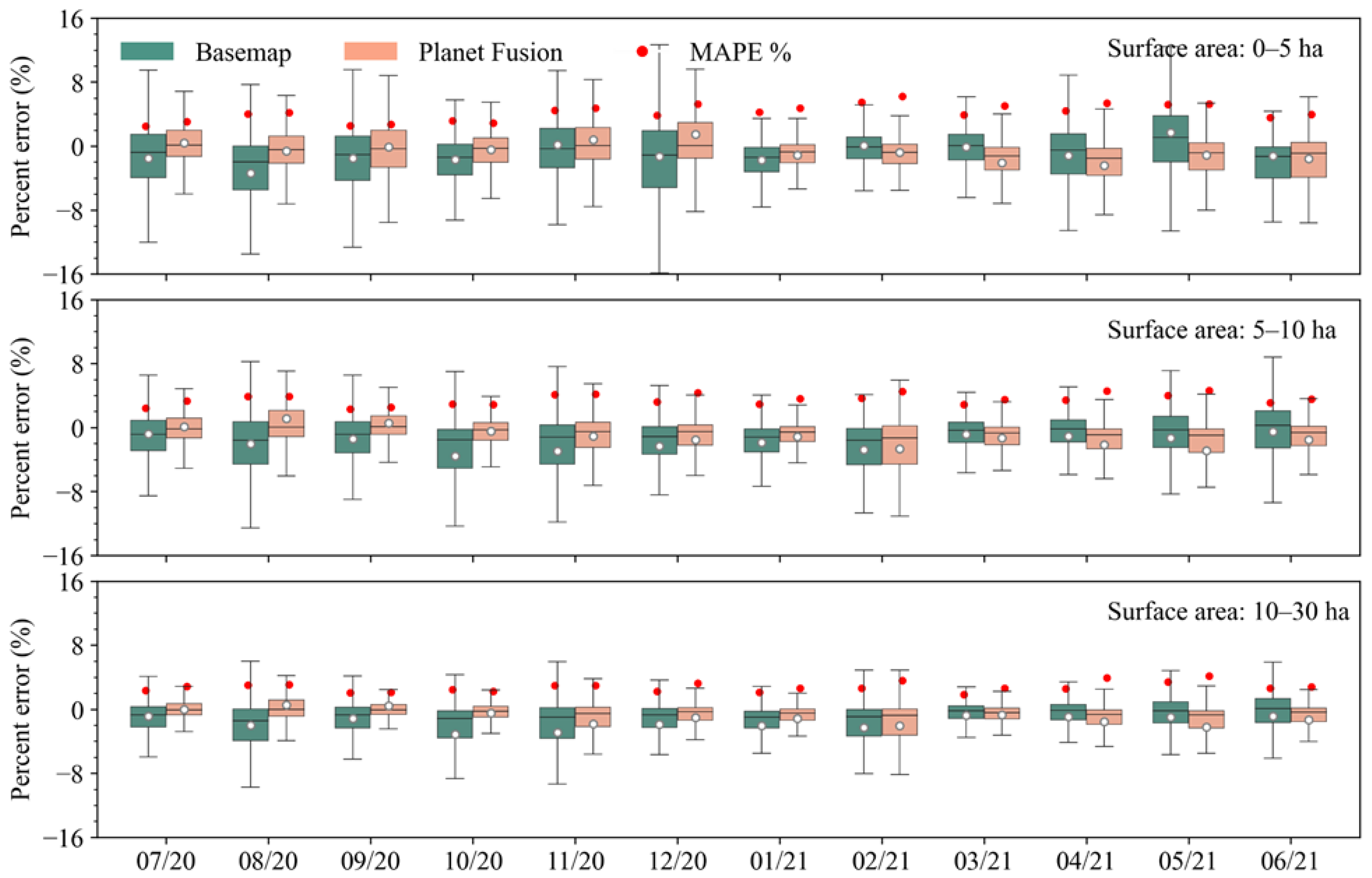
3.4. Monthly Comparisons between Basemap and Planet Fusion with PlanetScope
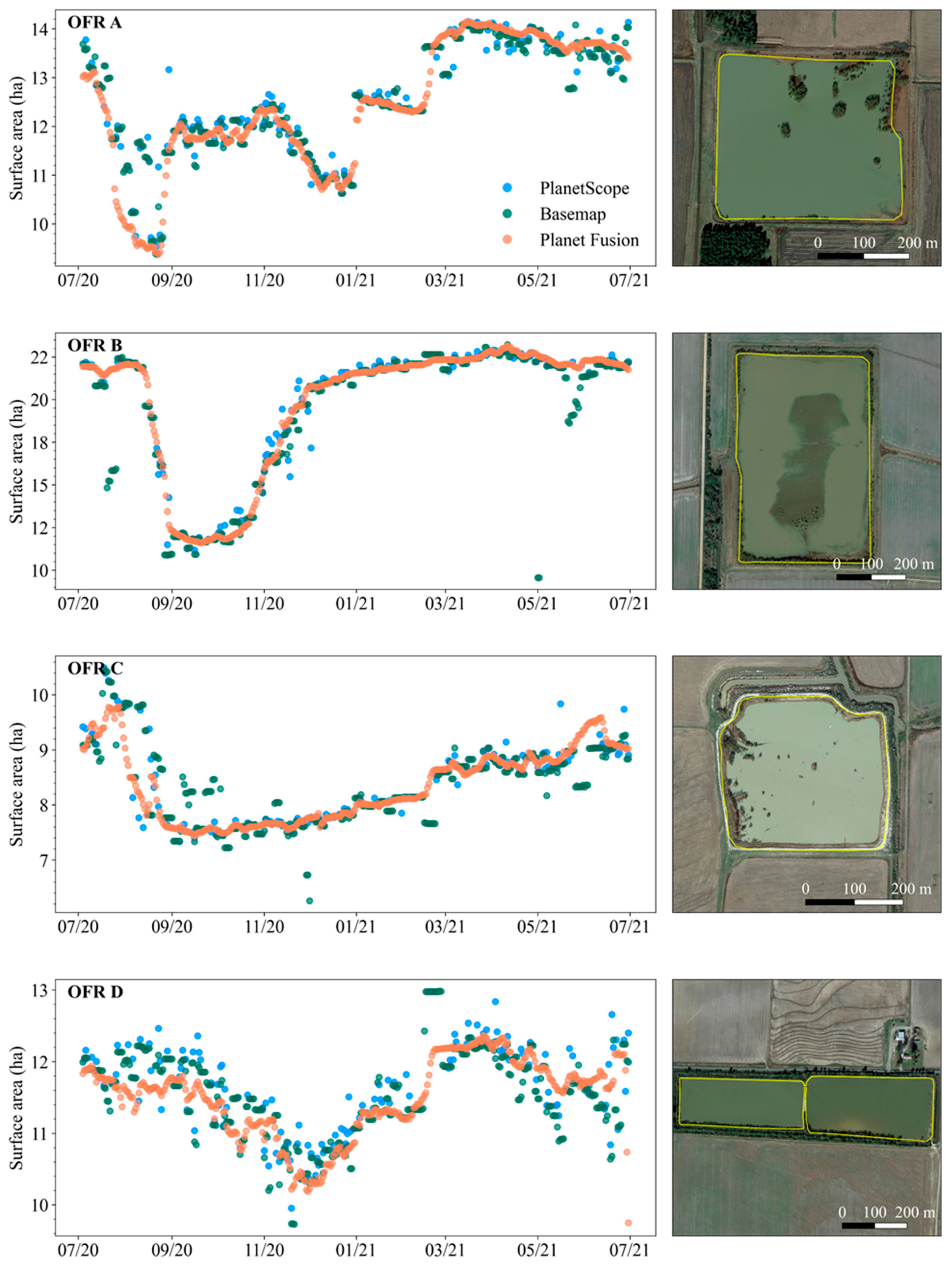
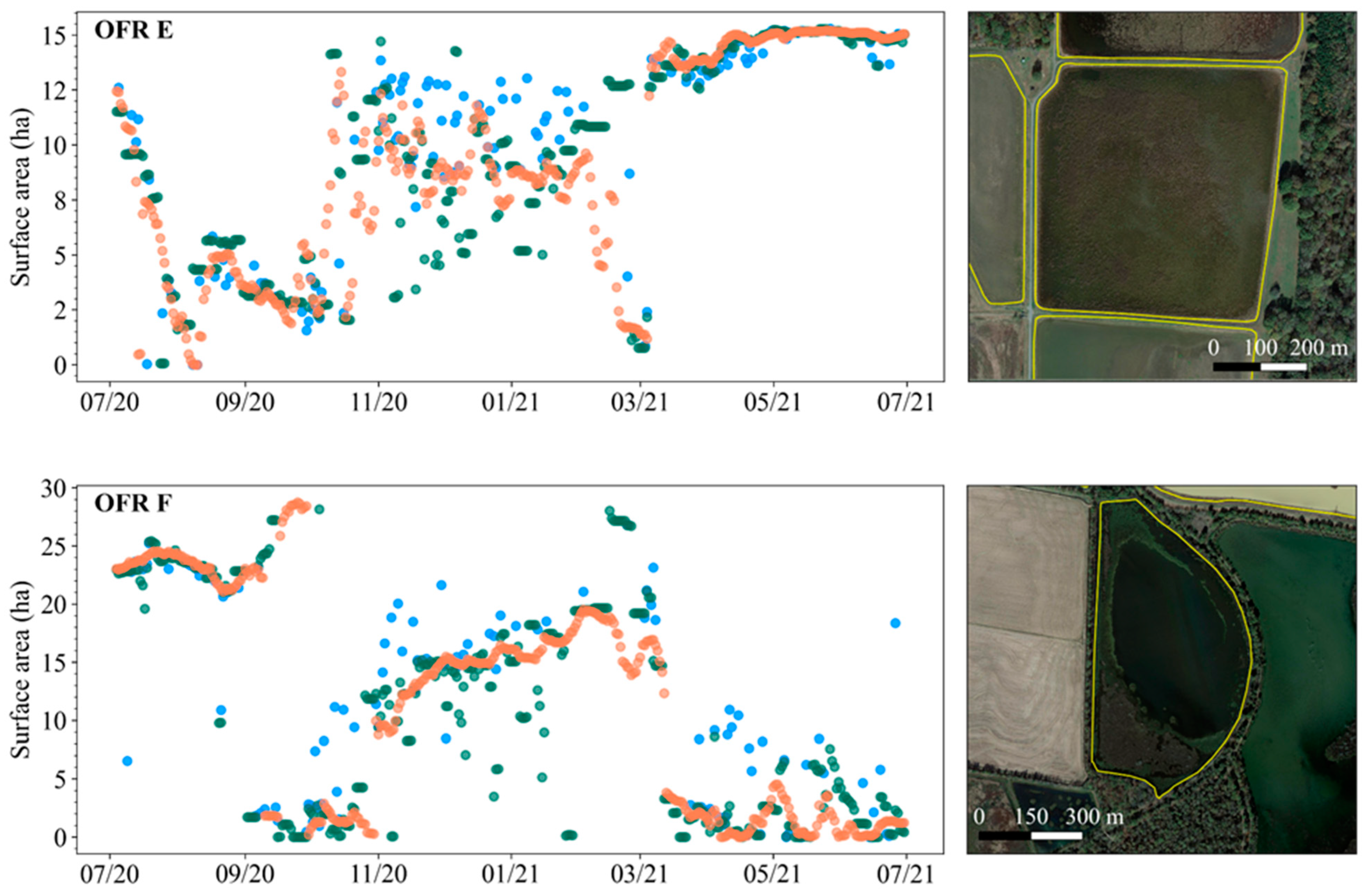
3.5. OFR Surface Area Time Series
4. Discussion
5. Known Issues and Limitations
6. Conclusions
Author Contributions
Funding
Acknowledgments
Conflicts of Interest
References
- Planet Team Planet Imagery Product Specifications. Available online: https://assets.planet.com/docs/Planet_Combined_Imagery_Product_Specs_letter_screen.pdf (accessed on 8 September 2021).
- Cooley, S.W.; Smith, L.C.; Stepan, L.; Mascaro, J. Tracking Dynamic Northern Surface Water Changes with High-Frequency Planet CubeSat Imagery. Remote Sens. 2017, 9, 1306. [Google Scholar] [CrossRef] [Green Version]
- Mishra, V.; Limaye, A.S.; Muench, R.E.; Cherrington, E.A.; Markert, K.N. Evaluating the performance of high-resolution satellite imagery in detecting ephemeral water bodies over West Africa. Int. J. Appl. Earth Obs. Geoinf. 2020, 93, 102218. [Google Scholar] [CrossRef]
- Vanthof, V.; Kelly, R. Water storage estimation in ungauged small reservoirs with the TanDEM-X DEM and multi-source satellite observations. Remote Sens. Environ. 2019, 235, 111437. [Google Scholar] [CrossRef]
- Hondula, K.L.; DeVries, B.; Jones, C.N.; Palmer, M.A. Effects of Using High Resolution Satellite-Based Inundation Time Series to Estimate Methane Fluxes From Forested Wetlands. Geophys. Res. Lett. 2021, 48, e2021GL092556. [Google Scholar] [CrossRef]
- Kääb, A.; Altena, B.; Mascaro, J. River-Ice and Water Velocities Using the Planet Optical Cubesat Constellation. Hydrol. Earth Syst. Sci. 2019, 23, 4233–4247. [Google Scholar] [CrossRef] [Green Version]
- Kimm, H.; Guan, K.; Jiang, C.; Peng, B.; Gentry, L.F.; Wilkin, S.C.; Wang, S.; Cai, Y.; Bernacchi, C.J.; Peng, J.; et al. Deriving High-Spatiotemporal-Resolution Leaf Area Index for Agroecosystems in the U.S. Corn Belt Using Planet Labs CubeSat and STAIR Fusion Data. Remote Sens. Environ. 2020, 239, 111615. [Google Scholar] [CrossRef]
- Houborg, R.; McCabe, M.F. A Cubesat Enabled Spatio-Temporal Enhancement Method (CESTEM) Utilizing Planet, Landsat and MODIS Data. Remote Sens. Environ. 2018, 209, 211–226. [Google Scholar] [CrossRef]
- Sadeh, Y.; Zhu, X.; Dunkerley, D.; Walker, J.P.; Zhang, Y.; Rozenstein, O.; Manivasagam, V.S.; Chenu, K. Fusion of Sentinel-2 and PlanetScope Time-Series Data into Daily 3 m Surface Reflectance and Wheat LAI Monitoring. Int. J. Appl. Earth Obs. Geoinf. 2021, 96, 102260. [Google Scholar] [CrossRef]
- Csillik, O.; Asner, G.P. Near-Real Time Aboveground Carbon Emissions in Peru. PLoS ONE 2020, 15, e0241418. [Google Scholar] [CrossRef]
- Csillik, O.; Kumar, P.; Mascaro, J.; O′Shea, T.; Asner, G.P. Monitoring Tropical Forest Carbon Stocks and Emissions Using Planet Satellite Data. Sci. Rep. 2019, 9, 17831. [Google Scholar] [CrossRef] [Green Version]
- Csillik, O.; Kumar, P.; Asner, G.P. Challenges in Estimating Tropical Forest Canopy Height from Planet Dove Imagery. Remote Sens. 2020, 12, 1160. [Google Scholar] [CrossRef] [Green Version]
- Roy, D.P.; Huang, H.; Houborg, R.; Martins, V.S. A Global Analysis of the Temporal Availability of PlanetScope High Spatial Resolution Multi-Spectral Imagery. Remote Sens. Environ. 2021, 264, 112586. [Google Scholar] [CrossRef]
- Cheng, Y.; Vrieling, A.; Fava, F.; Meroni, M.; Marshall, M.; Gachoki, S. Phenology of Short Vegetation Cycles in a Kenyan Rangeland from PlanetScope and Sentinel-2. Remote Sens. Environ. 2020, 248, 112004. [Google Scholar] [CrossRef]
- Wang, J.; Yang, D.; Chen, S.; Zhu, X.; Wu, S.; Bogonovich, M.; Guo, Z.; Zhu, Z.; Wu, J. Automatic Cloud and Cloud Shadow Detection in Tropical Areas for PlanetScope Satellite Images. Remote Sens. Environ. 2021, 264, 112604. [Google Scholar] [CrossRef]
- Planet Team Planet Basemaps Product Specification. Available online: https://assets.planet.com/products/basemap/planet-basemaps-product-specifications.pdf (accessed on 8 September 2021).
- Planet Team Planet Fusion Monitoring Technical Specification. Available online: https://assets.planet.com/docs/Planet_fusion_specification_March_2021.pdf (accessed on 8 September 2021).
- Kington, J.D.; Jordahl, K.A.; Kanwar, A.N.; Kapadia, A.; Schönert, M.; Wurster, K. IN13B-0716 Spatially and Temporally Consistent Smallsat-Derived Basemaps for Analytic Applications. In Proceedings of the American Geophysical Union, Fall Meeting 2019, San Francisco, CA, USA, 9–13 December 2019. [Google Scholar]
- Dadap, N.C.; Hoyt, A.M.; Cobb, A.R.; Oner, D.; Kozinski, M.; Fua, P.V.; Rao, K.; Harvey, C.F.; Konings, A.G. Drainage Canals in Southeast Asian Peatlands Increase Carbon Emissions. AGU Adv. 2021, 2, e2020AV000321. [Google Scholar] [CrossRef]
- Li, J.; Knapp, D.E.; Fabina, N.S.; Kennedy, E.V.; Larsen, K.; Lyons, M.B.; Murray, N.J.; Phinn, S.R.; Roelfsema, C.M.; Asner, G.P. A Global Coral Reef Probability Map Generated Using Convolutional Neural Networks. Coral Reefs 2020, 39, 1805–1815. [Google Scholar] [CrossRef]
- Kong, J.; Ryu, Y.; Huang, Y.; Dechant, B.; Houborg, R.; Guan, K.; Zhu, X. Evaluation of Four Image Fusion NDVI Products against In-Situ Spectral-Measurements over a Heterogeneous Rice Paddy Landscape. Agric. For. Meteorol. 2021, 297, 108255. [Google Scholar] [CrossRef]
- Houborg, R.; McCabe, M. Daily Retrieval of NDVI and LAI at 3 m Resolution via the Fusion of CubeSat, Landsat, and MODIS Data. Remote Sens. 2018, 10, 890. [Google Scholar] [CrossRef] [Green Version]
- Perin, V.; Tulbure, M.G.; Gaines, M.D.; Reba, M.L.; Yaeger, M.A. On-Farm Reservoir Monitoring Using Landsat Inundation Datasets. Agric. Water Manag. 2021, 246, 106694. [Google Scholar] [CrossRef]
- Habets, F.; Molénat, J.; Carluer, N.; Douez, O.; Leenhardt, D. The Cumulative Impacts of Small Reservoirs on Hydrology: A Review. Sci. Total Environ. 2018, 643, 850–867. [Google Scholar] [CrossRef] [Green Version]
- Fowler, K.; Morden, R.; Lowe, L.; Nathan, R. Advances in Assessing the Impact of Hillside Farm Dams on Streamflow. Australas. J. Water Resour. 2015, 19, 96–108. [Google Scholar] [CrossRef]
- Renwick, W.H.; Smith, S.V.; Bartley, J.D.; Buddemeier, R.W. The Role of Impoundments in the Sediment Budget of the Conterminous United States. Geomorphology 2005, 71, 99–111. [Google Scholar] [CrossRef]
- Downing, J.A. Emerging Global Role of Small Lakes and Ponds: Little Things Mean a Lot. Limnetica 2010, 29, 9–24. [Google Scholar] [CrossRef]
- Downing, J.A.; Prairie, Y.T.; Cole, J.J.; Duarte, C.M.; Tranvik, L.J.; Striegl, R.G.; McDowell, W.H.; Kortelainen, P.; Caraco, N.F.; Melack, J.M.; et al. The Global Abundance and Size Distribution of Lakes, Ponds, and Impoundments. Limnol. Oceanogr. 2006, 51, 2388–2397. [Google Scholar] [CrossRef] [Green Version]
- Habets, F.; Philippe, E.; Martin, E.; David, C.H.; Leseur, F. Small Farm Dams: Impact on River Flows and Sustainability in a Context of Climate Change. Hydrol. Earth Syst. Sci. 2014, 18, 4207–4222. [Google Scholar] [CrossRef] [Green Version]
- Mime, M.M.; Young, D.W. The Impact of Stockwatering Ponds (Stockponds) On Runoff from Large Arizona Watersheds. JAWRA J. Am. Water Resour. Assoc. 1989, 25, 165–173. [Google Scholar] [CrossRef]
- Jones, S.K.; Fremier, A.K.; DeClerck, F.A.; Smedley, D.; Pieck, A.O.; Mulligan, M. Big Data and Multiple Methods for Mapping Small Reservoirs: Comparing Accuracies for Applications in Agricultural Landscapes. Remote Sens. 2017, 9, 1307. [Google Scholar] [CrossRef] [Green Version]
- Ogilvie, A.; Belaud, G.; Massuel, S.; Mulligan, M.; Le Goulven, P.; Malaterre, P.-O.; Calvez, R. Combining Landsat Observations with Hydrological Modelling for Improved Surface Water Monitoring of Small Lakes. J. Hydrol. 2018, 566, 109–121. [Google Scholar] [CrossRef]
- Perin, V.; Tulbure, M.G.; Gaines, M.D.; Reba, M.L.; Yaeger, M.A. A Multi-Sensor Satellite Imagery Approach to Monitor on-Farm Reservoirs. Remote Sens. Environ. 2021, 112796. [Google Scholar] [CrossRef]
- Ogilvie, A.; Belaud, G.; Massuel, S.; Mulligan, M.; Le Goulven, P.; Calvez, R. Surface Water Monitoring in Small Water Bodies: Potential and Limits of Multi-Sensor Landsat Time Series. Hydrol. Earth Syst. Sci. 2018, 22, 4349–4380. [Google Scholar] [CrossRef] [Green Version]
- Yaeger, M.A.; Reba, M.L.; Massey, J.H.; Adviento-Borbe, M.A.A. On-Farm Irrigation Reservoirs in Two Arkansas Critical Groundwater Regions: A Comparative Inventory. Appl. Eng. Agric. 2017, 33, 869–878. [Google Scholar] [CrossRef]
- Yaeger, M.A.; Massey, J.H.; Reba, M.L.; Adviento-Borbe, M.A.A. Trends in the Construction of On-Farm Irrigation Reservoirs in Response to Aquifer Decline in Eastern Arkansas: Implications for Conjunctive Water Resource Management. Agric. Water Manag. 2018, 208, 373–383. [Google Scholar] [CrossRef]
- Shults, D.D.; Nowlin, W.J.; Yaeger, M.A.; Massey, J.H.; Reba, M.L. A Spatiotemporal Anlysis Quantifying the Need for More On-Farm Reservoirs to Reduce Groundwater Use in the Cache and L′Anguille River Regions in Northeaster AR. In Proceedings of the ESRI User Conference, Online, 13–16 July 2020. [Google Scholar]
- Kotchenova, S.Y.; Vermote, E.F.; Matarrese, R.; Klemm, F.J., Jr. Validation of a Vector Version of the 6S Radiative Transfer Code for Atmospheric Correction of Satellite Data Part I: Path Radiance. Appl. Opt. 2006, 45, 6762–6774. [Google Scholar] [CrossRef] [PubMed] [Green Version]
- Kotchenova, S.Y.; Vermote, E.F. Validation of a Vector Version of the 6S Radiative Transfer Code for Atmospheric Correction of Satellite Data Part II Homogeneous Lambertian and Anisotropic Surfaces. Appl. Opt. 2007, 46, 4455–4464. [Google Scholar] [CrossRef] [Green Version]
- Frantz, D. FORCE—Landsat + Sentinel-2 Analysis Ready Data and Beyond. Remote Sens. 2019, 11, 1124. [Google Scholar] [CrossRef] [Green Version]
- Tanre, D.; Deroo, C.; Duhaut, P.; Herman, M.; Morcrette, J.J.; Perbos, J.; Deschamps, P.Y. Technical Note Description of a Computer Code to Simulate the Satellite Signal in the Solar Spectrum: The 5S Code. Int. J. Remote Sens. 1990, 11, 659–668. [Google Scholar] [CrossRef]
- Zhu, Z.; Woodcock, C.E. Object-Based Cloud and Cloud Shadow Detection in Landsat Imagery. Remote Sens. Environ. 2012, 118, 83–94. [Google Scholar] [CrossRef]
- Frantz, D.; Haß, E.; Uhl, A.; Stoffels, J.; Hill, J. Improvement of the Fmask Algorithm for Sentinel-2 Images: Separating Clouds from Bright Surfaces Based on Parallax Effects. Remote Sens. Environ. 2018, 215, 471–481. [Google Scholar] [CrossRef]
- Planet Team Planet Basemaps: Comprehensive, High-Frequency Mosaics for Analysis. Available online: https://www.planet.com/products/basemap/ (accessed on 10 December 2021).
- Doxani, G.; Vermote, E.; Roger, J.-C.; Gascon, F.; Adriaensen, S.; Frantz, D.; Hagolle, O.; Hollstein, A.; Kirches, G.; Li, F.; et al. Atmospheric Correction Inter-Comparison Exercise. Remote Sens. 2018, 10, 352. [Google Scholar] [CrossRef] [PubMed] [Green Version]
- Schaaf, C.B.; Gao, F.; Strahler, A.H.; Lucht, W.; Li, X.; Tsang, T.; Strugnell, N.C.; Zhang, X.; Jin, Y.; Muller, J.-P.; et al. First Operational BRDF, Albedo Nadir Reflectance Products from MODIS. Remote Sens. Environ. 2002, 83, 135–148. [Google Scholar] [CrossRef] [Green Version]
- McFeeters, S.K. The Use of the Normalized Difference Water Index (NDWI) in the Delineation of Open Water Features. Int. J. Remote Sens. 1996, 17, 1425–1432. [Google Scholar] [CrossRef]
- Otsu, N. A Threshold Selection Method from Gray-Level Histograms. IEEE Trans. Syst. Man Cybern. 1979, 9, 62–66. [Google Scholar] [CrossRef] [Green Version]
- Du, Z.; Li, W.; Zhou, D.; Tian, L.; Ling, F.; Wang, H.; Gui, Y.; Sun, B. Analysis of Landsat-8 OLI Imagery for Land Surface Water Mapping. Remote Sens. Lett. 2014, 5, 672–681. [Google Scholar] [CrossRef]
- Li, J.; Wang, S. An Automatic Method for Mapping Inland Surface Waterbodies with Radarsat-2 Imagery. Int. J. Remote Sens. 2015, 36, 1367–1384. [Google Scholar] [CrossRef]
- Liu, Z.; Yao, Z.; Wang, R. Assessing Methods of Identifying Open Water Bodies Using Landsat 8 OLI Imagery. Environ. Earth Sci. 2016, 75, 873. [Google Scholar] [CrossRef]
- Sheng, Y.; Song, C.; Wang, J.; Lyons, E.A.; Knox, B.R.; Cox, J.S.; Gao, F. Representative Lake Water Extent Mapping at Continental Scales Using Multi-Temporal Landsat-8 Imagery. Remote Sens. Environ. 2016, 185, 129–141. [Google Scholar] [CrossRef] [Green Version]
- Wang, Z.; Zhang, R.; Zhang, Q.; Zhu, Y.; Huang, B.; Lu, Z. An Automatic Thresholding Method for Water Body Detection from SAR Image. In Proceedings of the 2019 IEEE International Conference on Signal, Information and Data Processing (ICSIDP), Chongqing, China, 11–13 December 2019; pp. 1–4. [Google Scholar]
- Gorelick, N.; Hancher, M.; Dixon, M.; Ilyushchenko, S.; Thau, D.; Moore, R. Google Earth Engine: Planetary-Scale Geospatial Analysis for Everyone. Remote Sens. Environ. 2017, 202, 18–27. [Google Scholar] [CrossRef]
- DeVries, B.; Huang, C.; Lang, M.; Jones, J.; Huang, W.; Creed, I.; Carroll, M. Automated Quantification of Surface Water Inundation in Wetlands Using Optical Satellite Imagery. Remote Sens. 2017, 9, 807. [Google Scholar] [CrossRef] [Green Version]
- Avisse, N.; Tilmant, A.; Müller, M.F.; Zhang, H. Monitoring Small Reservoirs′ Storage with Satellite Remote Sensing in Inaccessible Areas. Hydrol. Earth Syst. Sci. 2017, 21, 6445–6459. [Google Scholar] [CrossRef] [Green Version]
- López-Caloca, A.A.; Escalante-Ramírez, B.; Henao, P. Mapping Small and Medium-Sized Water Reservoirs Using Sentinel-1A: A Case Study in Chiapas, Mexico. J. Appl. Remote Sens. 2020, 14, 036503. [Google Scholar] [CrossRef]
- Pena-Regueiro, J.; Sebastiá-Frasquet, M.-T.; Estornell, J.; Aguilar-Maldonado, J.A. Sentinel-2 Application to the Surface Characterization of Small Water Bodies in Wetlands. Water 2020, 12, 1487. [Google Scholar] [CrossRef]
- Yang, X.; Zhao, S.; Qin, X.; Zhao, N.; Liang, L. Mapping of Urban Surface Water Bodies from Sentinel-2 MSI Imagery at 10 m Resolution via NDWI-Based Image Sharpening. Remote Sens. 2017, 9, 596. [Google Scholar] [CrossRef] [Green Version]
- Yang, X.; Qin, Q.; Yésou, H.; Ledauphin, T.; Koehl, M.; Grussenmeyer, P.; Zhu, Z. Monthly Estimation of the Surface Water Extent in France at a 10-m Resolution Using Sentinel-2 Data. Remote Sens. Environ. 2020, 244, 111803. [Google Scholar] [CrossRef]
- Yao, F.; Wang, J.; Yang, K.; Wang, C.; Walter, B.A.; Crétaux, J.F. Lake Storage Variation on the Endorheic Tibetan Plateau and Its Attribution to Climate Change since the New Millennium. Environ. Res. Lett. 2018, 13, 064011. [Google Scholar] [CrossRef]
- Zhang, S.; Foerster, S.; Medeiros, P.; de Araújo, J.C.; Motagh, M.; Waske, B. Bathymetric Survey of Water Reservoirs in North-Eastern Brazil Based on TanDEM-X Satellite Data. Sci. Total Environ. 2016, 571, 575–593. [Google Scholar] [CrossRef] [PubMed]
- Hughes, D.A.; Mantel, S.K. Estimation Des Incertitudes Lors de La Simulation Des Impacts de Petites Retenues Agricoles Sur Les Régimes d′écoulement En Afrique Du Sud. Hydrol. Sci. J. 2010, 55, 578–592. [Google Scholar] [CrossRef]
- Ahmad, S.K.; Hossain, F.; Eldardiry, H.; Pavelsky, T.M. A Fusion Approach for Water Area Classification Using Visible, Near Infrared and Synthetic Aperture Radar for South Asian Conditions. IEEE Trans. Geosci. Remote Sens. 2020, 58, 2471–2480. [Google Scholar] [CrossRef]


| Source | Pixel Size (m) | Blue (µm) | Green (µm) | Red (µm) | NIR (µm) |
|---|---|---|---|---|---|
| PlanetScope | 3 | 0.455–0.515 | 0.500–0.590 | 0.590–0.670 | 0.780–0.860 |
| Basemap | 3 | 0.450–0.510 | 0.530–0.590 | 0.640–0.670 | 0.850–0.860 |
| Planet Fusion | 3 | 0.450–0.510 | 0.530–0.590 | 0.640–0.670 | 0.850–0.880 |
| OFR id | OFR Size (ha) |
|---|---|
| A | 13.62 |
| B | 22.60 |
| C | 9.83 |
| D | 12.73 |
| E | 13.82 |
| F | 29.72 |
| SkySat Image | Date | OFRs Observations | Percent Clear (%) | Ground-Control Ratio | Ground Sampling Distance (m) |
|---|---|---|---|---|---|
| 20200929_193409_ssc10_u0001 | 29 September 2020 | 35 | 87 | 0.91 | 0.66 |
| 20201013_194518_ssc6_u0001 | 13 October 2020 | 44 | 99 | 0.97 | 0.73 |
| 20201102_193752_ssc9_u0001 | 2 November 2020 | 16 | 100 | 0.97 | 0.67 |
| 20201102_193752_ssc9_u0002 | 2 November 2020 | 10 | 100 | 0.96 | 0.67 |
| 20201210_194154_ssc11_u0001 | 10 December 2020 | 39 | 99 | 0.91 | 0.68 |
| PlanetScope | Basemap | Planet Fusion | |||||||
|---|---|---|---|---|---|---|---|---|---|
| 0.1–5 ha | 5–10 ha | 10–30 ha | 0.1–5 ha | 5–10 ha | 10–30 ha | 0.1–5 ha | 5–10 ha | 10–30 ha | |
| r2 | 0.91 | 0.91 | 0.94 | 0.91 | 0.87 | 0.90 | 0.96 | 0.96 | 0.95 |
| MAPE (%) | 7.05 | 7.14 | 7.68 | 9.91 | 10.1 | 10.8 | 7.37 | 7.46 | 9.11 |
Publisher’s Note: MDPI stays neutral with regard to jurisdictional claims in published maps and institutional affiliations. |
© 2021 by the authors. Licensee MDPI, Basel, Switzerland. This article is an open access article distributed under the terms and conditions of the Creative Commons Attribution (CC BY) license (https://creativecommons.org/licenses/by/4.0/).
Share and Cite
Perin, V.; Roy, S.; Kington, J.; Harris, T.; Tulbure, M.G.; Stone, N.; Barsballe, T.; Reba, M.; Yaeger, M.A. Monitoring Small Water Bodies Using High Spatial and Temporal Resolution Analysis Ready Datasets. Remote Sens. 2021, 13, 5176. https://doi.org/10.3390/rs13245176
Perin V, Roy S, Kington J, Harris T, Tulbure MG, Stone N, Barsballe T, Reba M, Yaeger MA. Monitoring Small Water Bodies Using High Spatial and Temporal Resolution Analysis Ready Datasets. Remote Sensing. 2021; 13(24):5176. https://doi.org/10.3390/rs13245176
Chicago/Turabian StylePerin, Vinicius, Samapriya Roy, Joe Kington, Thomas Harris, Mirela G. Tulbure, Noah Stone, Torben Barsballe, Michele Reba, and Mary A. Yaeger. 2021. "Monitoring Small Water Bodies Using High Spatial and Temporal Resolution Analysis Ready Datasets" Remote Sensing 13, no. 24: 5176. https://doi.org/10.3390/rs13245176