
Quantifying the Variability of Phytoplankton Blooms in the NW Mediterranean Sea with the Robust Satellite Techniques (RST)

 ,
,  , , , ,
Abstract
:1. Introduction
2. Materials and Methods
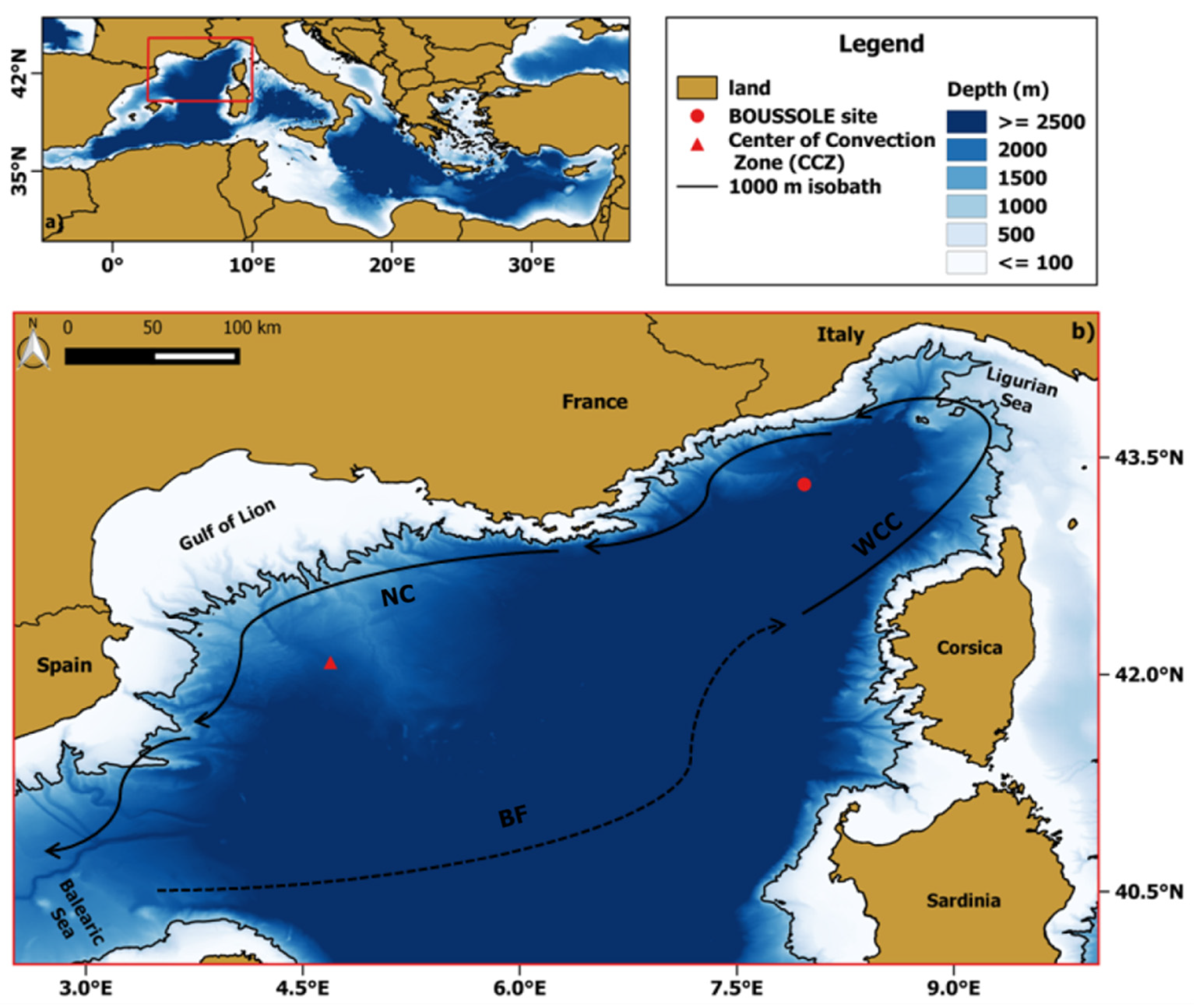
2.1. Study Area
2.2. In Situ Chl-A Data
2.3. Satellite Chl-A Data
2.4. The Robust Satellite Techniques
2.5. Ancillary Data
2.6. Match-Up Analysis
3. Results
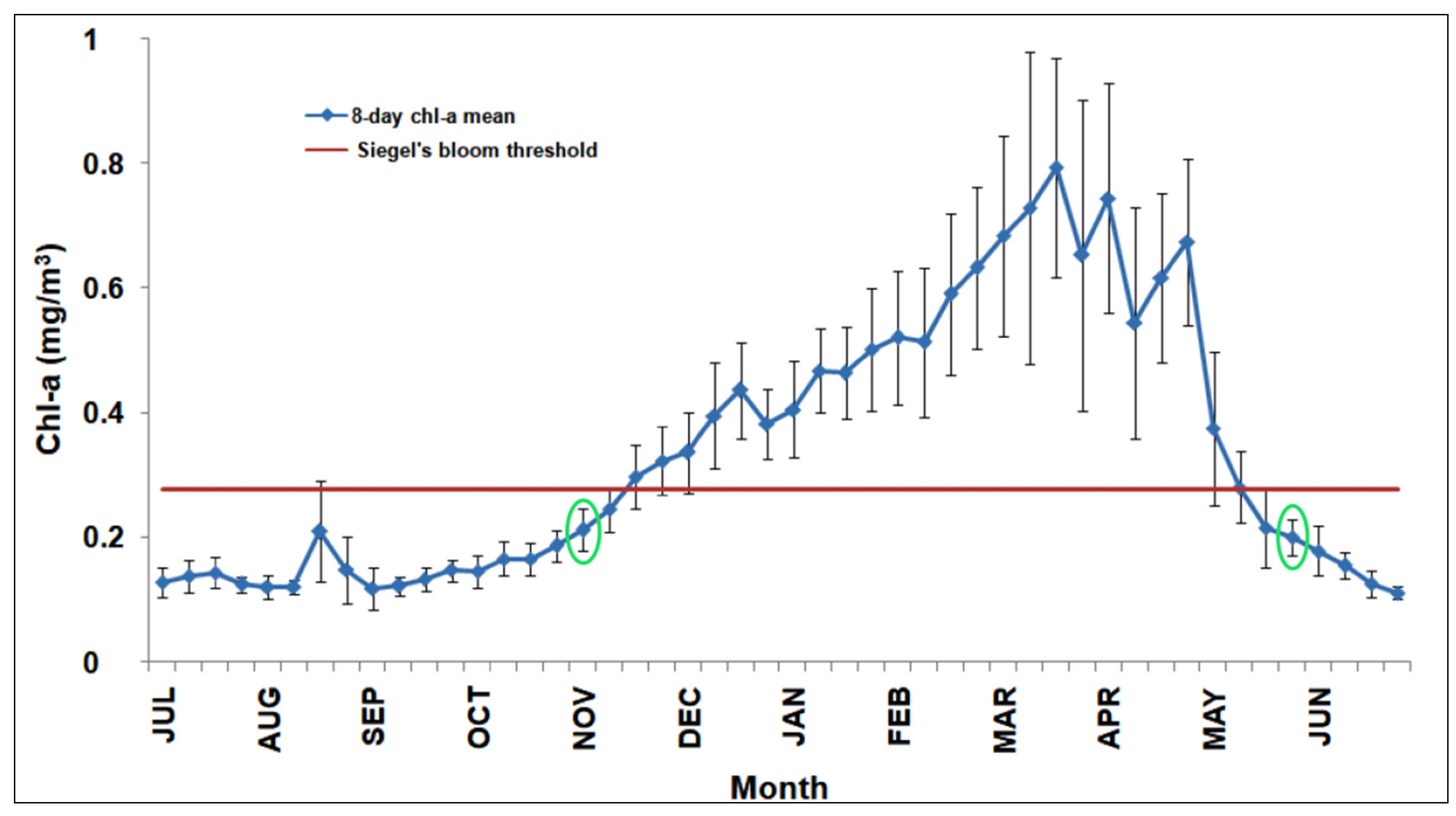
3.1. Climatological Analysis
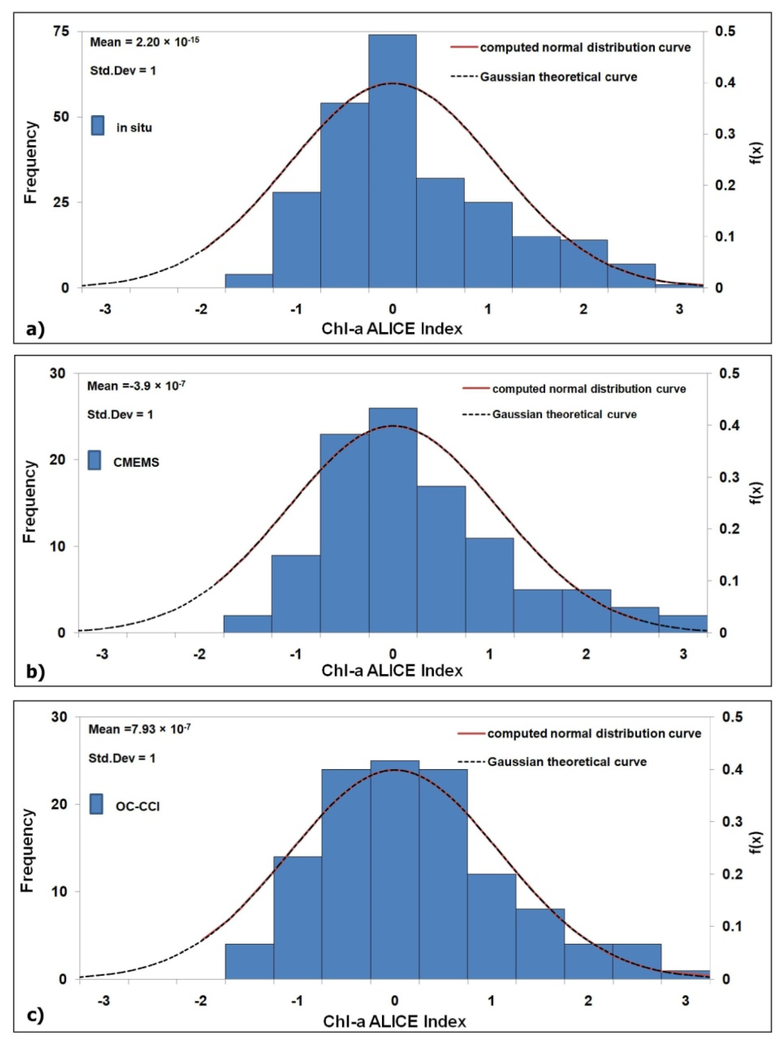
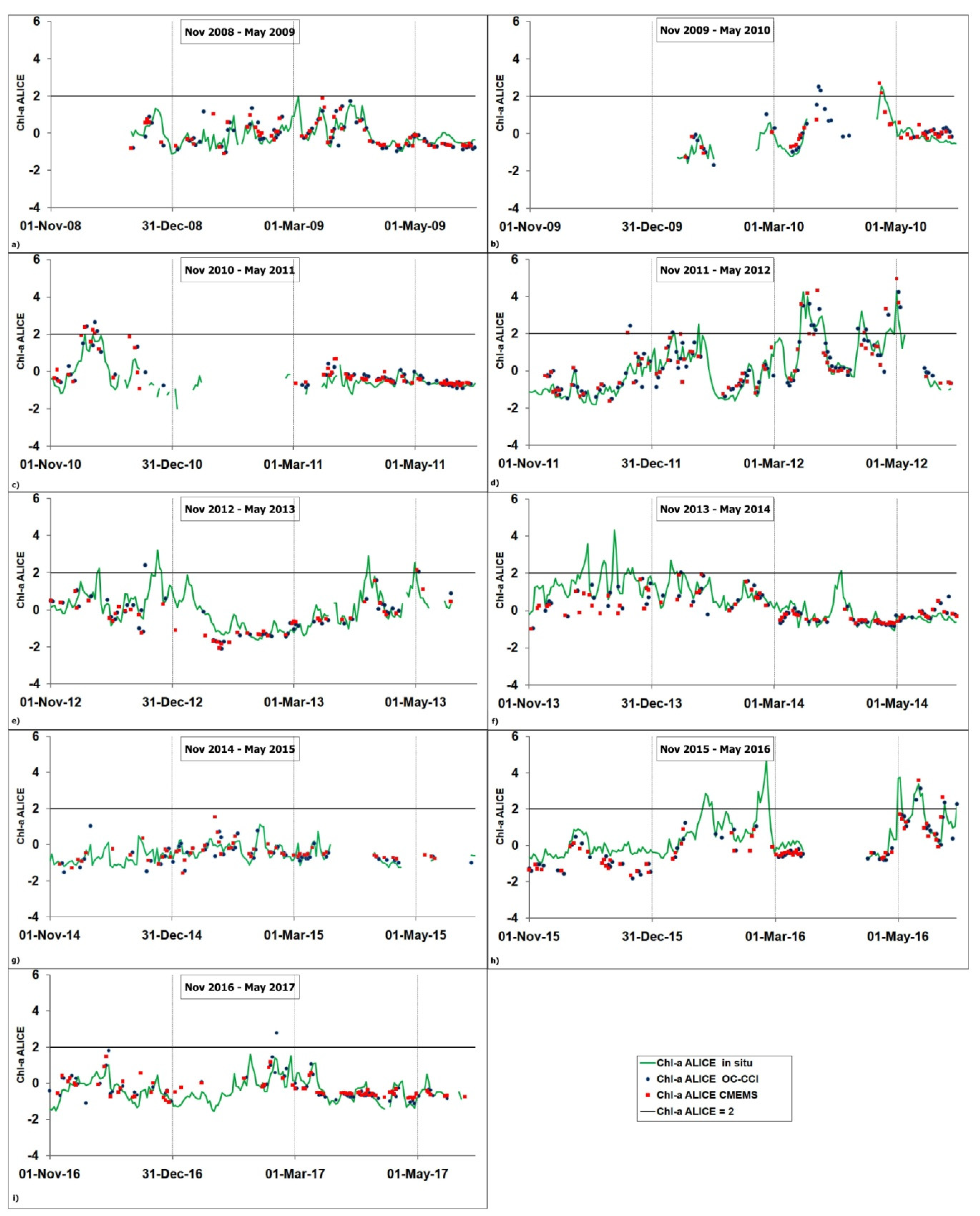
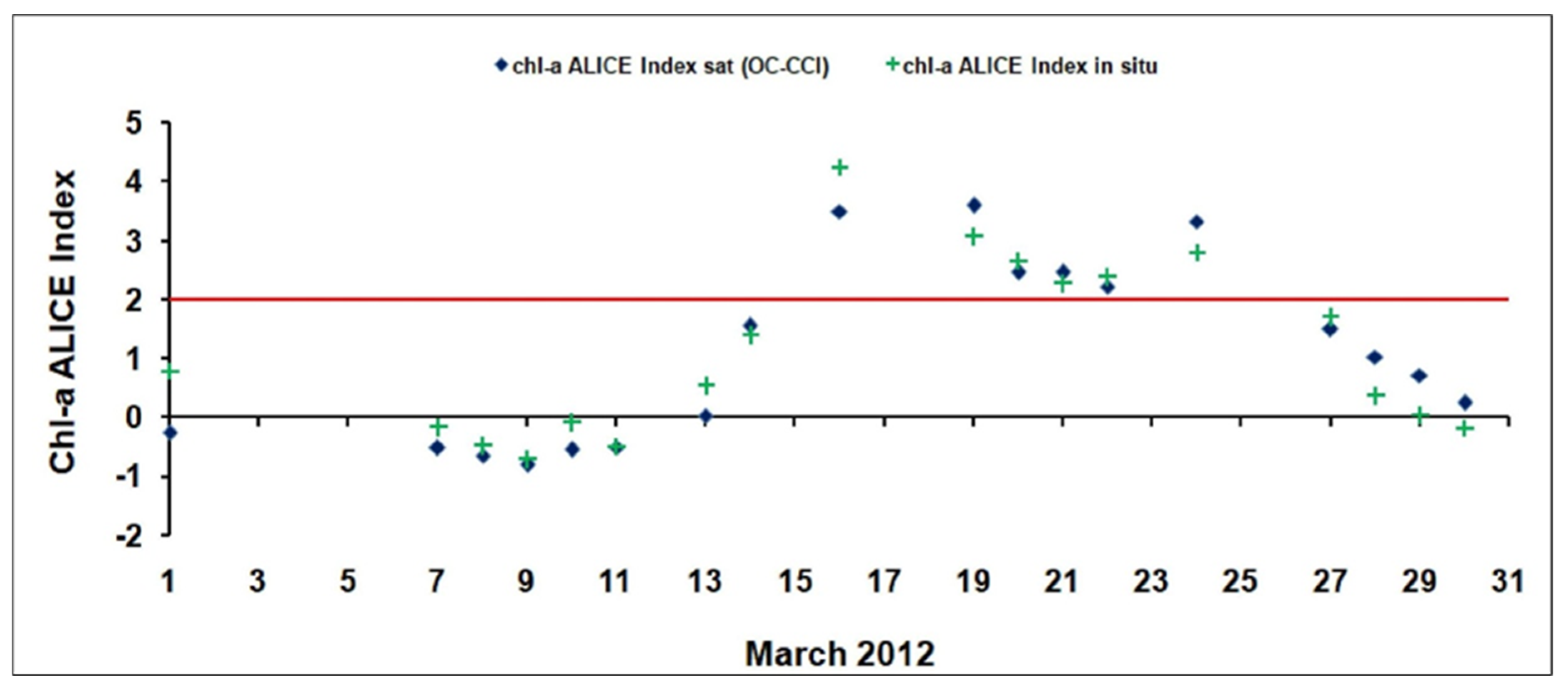
3.2. Validation of the Satellite Chl-A Absolutely Local Index of Change of the Environment(ALICE)
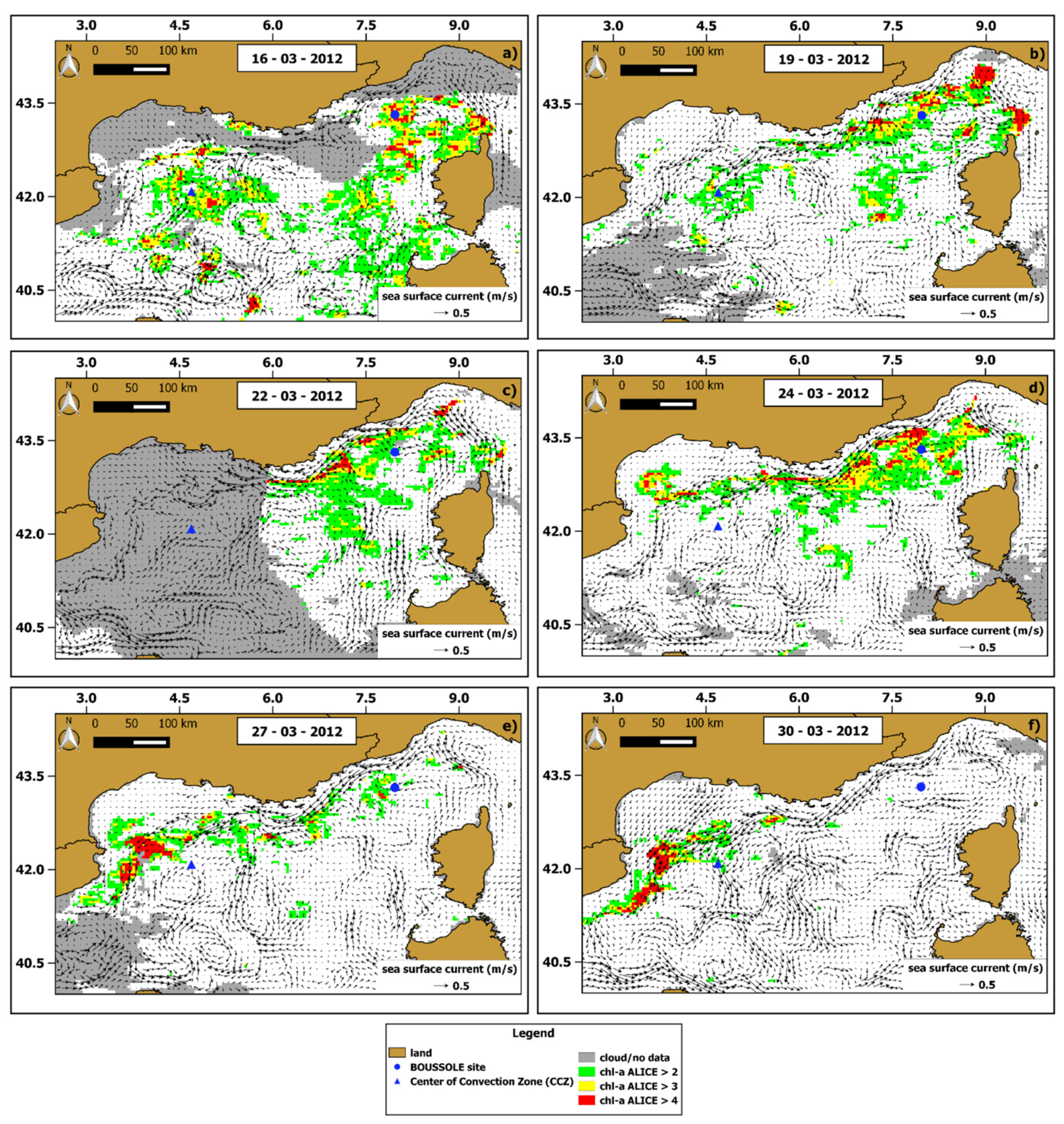
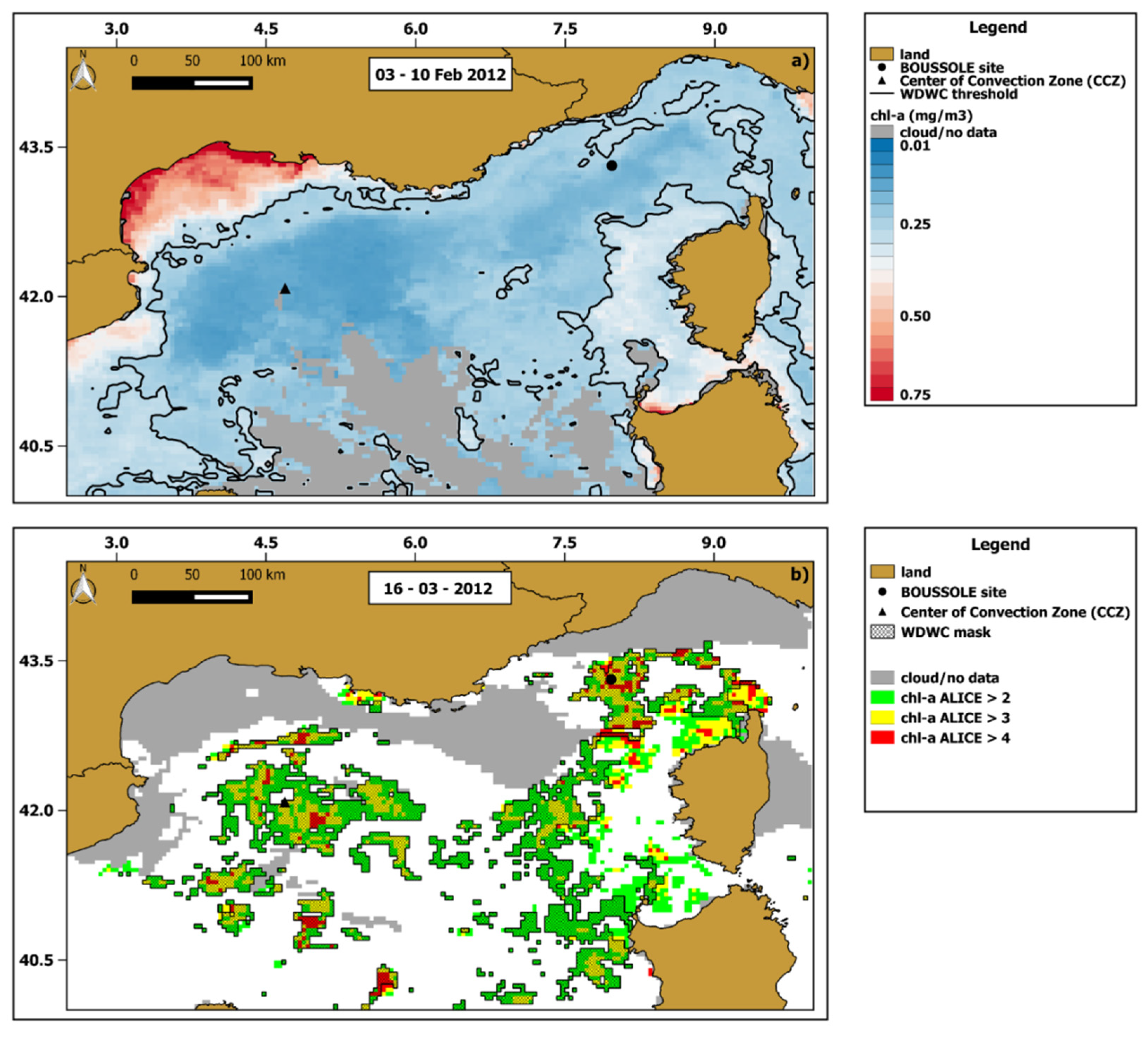
3.3. Regional Scale Analysis: The March 2012 Case Study
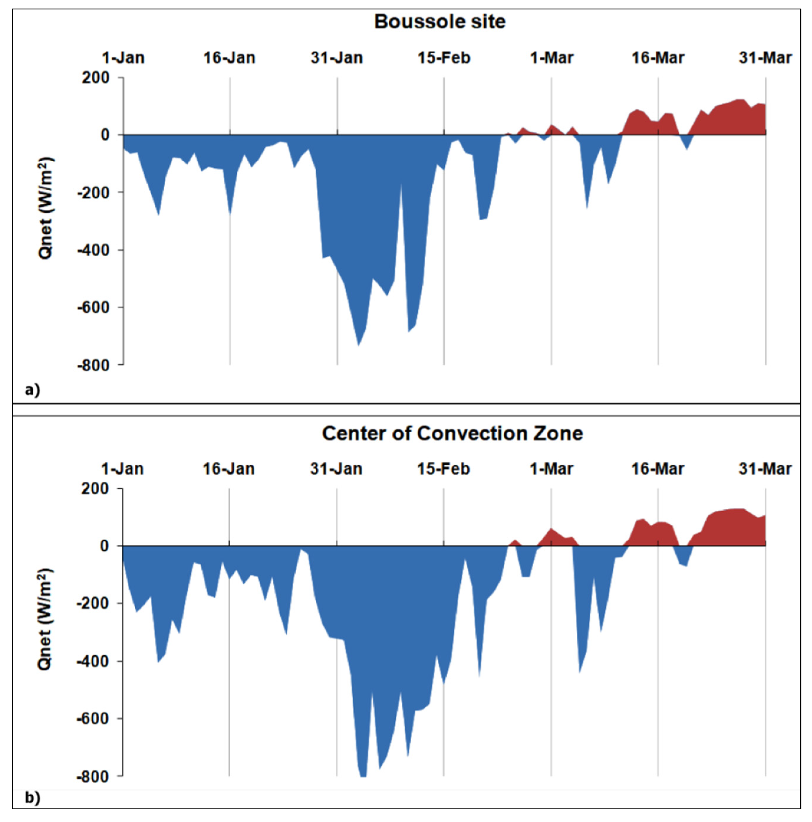
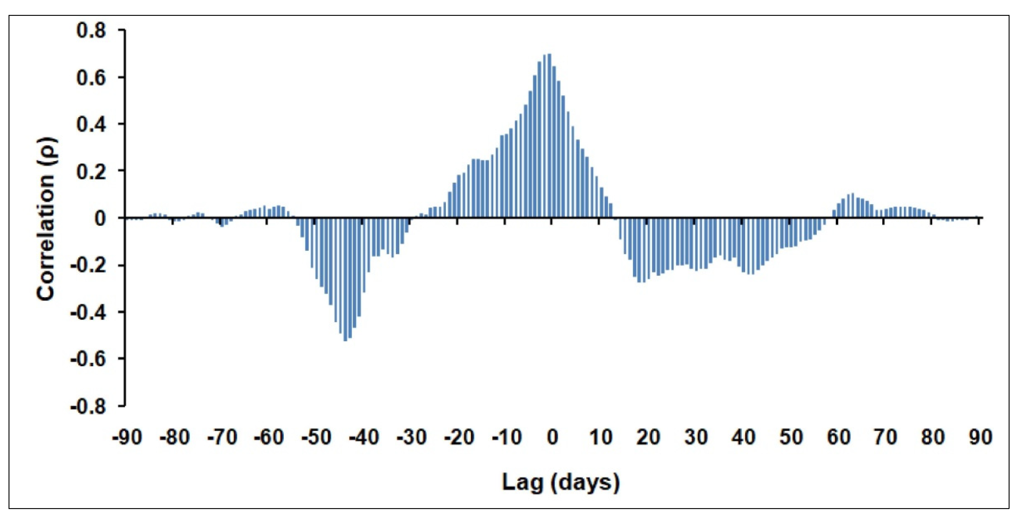
3.4. Influence of Winter Deep Water Convection (WDWC)Event on the March 2012 Anomalous Chl-A Bloom
4. Conclusions
Author Contributions
Funding
Acknowledgments
Conflicts of Interest
Appendix A


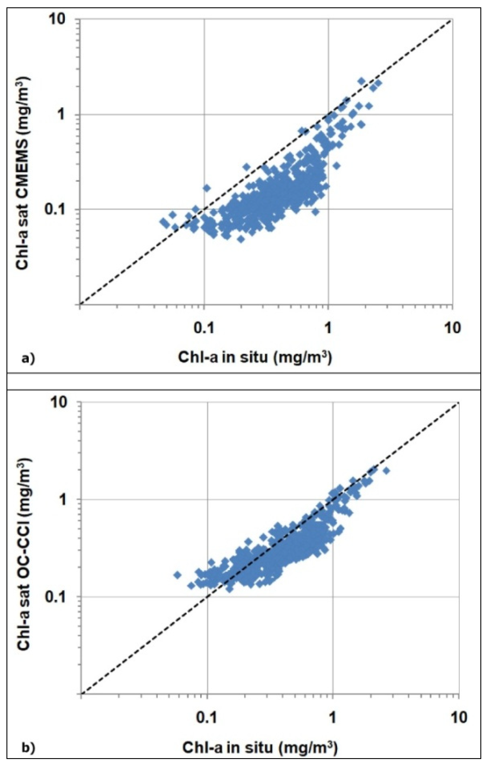
| Chl-A Algorithm | N | R2 | p-Value | RMSE (g/m3) |
|---|---|---|---|---|
| CMEMS | 550 | 0.66 | <0.001 | 0.33 |
| OC-CCI | 588 | 0.80 | <0.001 | 0.18 |
| Dataset | Water Type | Membership (%) |
|---|---|---|
| CMEMS | Case I | 96.36 |
| Case II | 3.64 | |
| OC-CCI | Open | 12.76 |
| Transitional | 86.89 | |
| Coastal | 0.35 |
References
- Devred, E.; Sathyendranath, S.; Platt, T. Decadal changes in ecological provinces of the Northwest Atlantic Ocean revealed by satellite observations. Geophys. Res. Lett. 2009, 36. [Google Scholar] [CrossRef]
- Brewin, R.J.; Hirata, T.; Hardman-Mountford, N.J.; Lavender, S.J.; Sathyendranath, S.; Barlow, R. The influence of the Indian Ocean Dipole on interannual variations in phytoplankton size structure as revealed by Earth Observation. Deep Sea Res. Part II Top. Stud. Oceanogr. 2012, 77–80, 117–127. [Google Scholar] [CrossRef]
- Racault, M.-F.; Sathyendranath, S.; Menon, N.; Platt, T. Phenological Responses to ENSO in the Global Oceans. Surv. Geophys. 2017, 38, 277–293. [Google Scholar] [CrossRef] [PubMed] [Green Version]
- Edwards, M.; Richardson, A.J. Impact of climate change on marine pelagic phenology and trophic mismatch. Nature 2004, 430, 881–884. [Google Scholar] [CrossRef] [PubMed]
- Platt, T.; Fuentes-Yaco, C.; Frank, K.T. Spring algal bloom and larval fish survival. Nature 2003, 423, 398–399. [Google Scholar] [CrossRef] [PubMed]
- Ferreira, A.; Brotas, V.; Palma, C.; Borges, C.; Brito, A.C. Assessing Phytoplankton Bloom Phenology in Upwelling-Influenced Regions Using Ocean Color Remote Sensing. Remote Sens. 2021, 13, 675. [Google Scholar] [CrossRef]
- Salgado-Hernanz, P.M.; Racault, M.F.; Font-Muñoz, J.S.; Basterretxea, G. Trends in phytoplankton phenology in the Mediterranean Sea based on ocean-colour remote sensing. Remote Sens. Environ. 2019, 221, 50–64. [Google Scholar] [CrossRef]
- Lacava, T.; Ciancia, E. Remote Sensing Applications in Coastal Areas. Sensors 2020, 20, 2673. [Google Scholar] [CrossRef] [PubMed]
- Ciancia, E.; Loureiro, C.M.; Mendonça, A.; Coviello, I.; Di Polito, C.; Lacava, T.; Pergola, N.; Satriano, V.; Tramutoli, V.; Martins, A. On the potential of an RST-based analysis of the MODIS-derived chl-a product over Condor seamount and surrounding areas (Azores, NE Atlantic). Ocean Dyn. 2016, 66, 1165–1180. [Google Scholar] [CrossRef]
- D’Ortenzio, F.; Ribera d’Alcalà, M. On the trophic regimes of the Mediterranean Sea: A satellite analysis. Biogeosciences 2009, 6, 139–148. [Google Scholar] [CrossRef] [Green Version]
- Mélin, F.; Vantrepotte, V.; Clerici, M.; D’Alimonte, D.; Zibordi, G.; Berthon, J.-F.; Canuti, E. Multi-sensor satellite time series of optical properties and chlorophyll-a concentration in the Adriatic Sea. Prog. Oceanogr. 2011, 91, 229–244. [Google Scholar] [CrossRef]
- Ayata, S.-D.; Irisson, J.-O.; Aubert, A.; Berline, L.; Dutay, J.-C.; Mayot, N.; Nieblas, A.-E.; D’Ortenzio, F.; Palmieri, J.; Reygondeau, G.; et al. Regionalisation of the Mediterranean basin, a MERMEX synthesis. Prog. Oceanogr. 2018, 163, 7–20. [Google Scholar] [CrossRef] [Green Version]
- Basterretxea, G.; Font-Muñoz, J.S.; Salgado-Hernanz, P.M.; Arrieta, J.; Hernández-Carrasco, I. Patterns of chlorophyll interannual variability in Mediterranean biogeographical regions. Remote Sen. Environ. 2018, 215, 7–17. [Google Scholar] [CrossRef]
- Keerthi, M.G.; Levy, M.; Aumont, O.; Lengaigne, M.; Antoine, D. Contrasted Contribution of Intraseasonal Time Scales to Surface Chlorophyll Variations in a Bloom and an Oligotrophic Regime. J. Geophys. Res. Oceans 2020, 125, e2019JC015701. [Google Scholar] [CrossRef]
- Barale, V.; Jaquet, J.-M.; Ndiaye, M. Algal blooming patterns and anomalies in the Mediterranean Sea as derived from the SeaWiFS data set (1998–2003). Remote Sens. Environ. 2008, 112, 3300–3313. [Google Scholar] [CrossRef]
- Mayot, N.; D’Ortenzio, F.; Ribera d’Alcalà, M.; Lavigne, H.; Claustre, H. Interannual variability of the Mediterranean trophic regimes from ocean color satellites. Biogeosciences 2016, 13, 1901–1917. [Google Scholar] [CrossRef] [Green Version]
- Volpe, G.; Nardelli, B.B.; Cipollini, P.; Santoleri, R.; Robinson, I.S. Seasonal to interannual phytoplankton response to physical processes in the Mediterranean Sea from satellite observations. Remote Sens. Environ. 2012, 117, 223–235. [Google Scholar] [CrossRef]
- Vantrepotte, V.; Mélin, F. Temporal variability of 10-year global SeaWiFS time-series of phytoplankton chlorophyll a concentration. ICES J. Mar. Sci. 2009, 66, 1547–1556. [Google Scholar] [CrossRef] [Green Version]
- Taylor, J.R.; Ferrari, R. Shutdown of turbulent convection as a new criterion for the onset of spring phytoplankton blooms. Limnol. Oceanogr. 2011, 56, 2293–2307. [Google Scholar] [CrossRef] [Green Version]
- Heimbürger, L.-E.; Lavigne, H.; Migon, C.; D’Ortenzio, F.; Estournel, C.; Coppola, L.; Miquel, J.-C. Temporal variability of vertical export flux at the DYFAMED time-series station (Northwestern Mediterranean Sea). Prog. Oceanogr. 2013, 119, 59–67. [Google Scholar] [CrossRef]
- Herrmann, M.; Diaz, F.; Estournel, C.; Marsaleix, P.; Ulses, C. Impact of atmospheric and oceanic interannual variability on the Northwestern Mediterranean Sea pelagic planktonic ecosystem and associated carbon cycle. J. Geophys. Res. Oceans 2013, 118, 5792–5813. [Google Scholar] [CrossRef]
- Estrada, M.; Latasa, M.; Emelianov, M.; Gutiérrez-Rodríguez, A.; Fernández-Castro, B.; Isern-Fontanet, J.; Mouriño-Carballido, B.; Salat, J.; Vidal, M. Seasonal and mesoscale variability of primary production in the deep winter-mixing region of the NW Mediterranean. Deep Sea Res. Part I Oceanogr. Res. Pap. 2014, 94, 45–61. [Google Scholar] [CrossRef]
- Mayot, N.; D’Ortenzio, F.; Taillandier, V.; Prieur, L.; De Fommervault, O.P.; Claustre, H.; Bosse, A.; Testor, P.; Conan, P. Physical and Biogeochemical Controls of the Phytoplankton Blooms in North Western Mediterranean Sea: A Multiplatform Approach Over a Complete Annual Cycle (2012–2013 DEWEX Experiment). J. Geophys. Res. Oceans 2017, 122, 9999–10019. [Google Scholar] [CrossRef]
- Macias, D.; Garcia-Gorriz, E.; Stips, A. Deep winter convection and phytoplankton dynamics in the NW Mediterranean Sea under present climate and future (horizon 2030) scenarios. Sci. Rep. 2018, 8, 6626. [Google Scholar] [CrossRef]
- Colella, S.; Falcini, F.; Rinaldi, E.; Sammartino, M.; Santoleri, R. Mediterranean Ocean Colour Chlorophyll Trends. PLoS ONE 2016, 11, e0155756. [Google Scholar] [CrossRef] [PubMed] [Green Version]
- Sathyendranath, S.; Brewin, R.J.; Jackson, T.; Mélin, F.; Platt, T. Ocean-colour products for climate-change studies: What are their ideal characteristics? Remote Sens. Environ. 2017, 203, 125–138. [Google Scholar] [CrossRef] [Green Version]
- Tramutoli, V. Robust Satellite Techniques (RST) for Natural and Environmental Hazards Monitoring and Mitigation: Theory and Applications. In Proceedings of the Fourth International Workshop on the Analysis of Multi-temporal Remote Sensing Images, Leuven, Belgium, 18–20 July 2007; pp. 1–6. [Google Scholar]
- Di Polito, C.; Ciancia, E.; Coviello, I.; Doxaran, D.; Lacava, T.; Pergola, N.; Satriano, V.; Tramutoli, V. On the Potential of Robust Satellite Techniques Approach for SPM Monitoring in Coastal Waters: Implementation and Application over the Basilicata Ionian Coastal Waters Using MODIS-Aqua. Remote Sens. 2016, 8, 922. [Google Scholar] [CrossRef] [Green Version]
- Lacava, T.; Ciancia, E.; Coviello, I.; Di Polito, C.; Grimaldi, C.S.L.; Pergola, N.; Satriano, V.; Temimi, M.; Zhao, J.; Tramutoli, V. A MODIS-Based Robust Satellite Technique (RST) for Timely Detection of Oil Spilled Areas. Remote Sens. 2017, 9, 128. [Google Scholar] [CrossRef] [Green Version]
- Ciancia, E.; Coviello, I.; Di Polito, C.; Lacava, T.; Pergola, N.; Satriano, V.; Tramutoli, V. Investigating the chlorophyll-a variability in the Gulf of Taranto (North-western Ionian Sea) by a multi-temporal analysis of MODIS-Aqua Level 3/Level 2 data. Cont. Shelf Res. 2018, 155, 34–44. [Google Scholar] [CrossRef]
- Franz, B.A.; Kwiatowska, E.J.; Meister, G.; McClain, C.R. Moderate Resolution Imaging Spectroradiometer on Terra: Limitations for ocean color applications. J. Appl. Remote Sens. 2008, 2, 023525. [Google Scholar] [CrossRef]
- Volpe, G.; Colella, S.; Brando, V.E.; Forneris, V.; La Padula, F.; Di Cicco, A.; Sammartino, M.; Bracaglia, M.; Artuso, F.; Santoleri, R. Mediterranean ocean colour Level 3 operational multi-sensor processing. Ocean Sci. 2019, 15, 127–146. [Google Scholar] [CrossRef] [Green Version]
- Sathyendranath, S.; Brewin, R.J.; Brockmann, C.; Brotas, V.; Calton, B.; Chuprin, A.; Cipollini, P.; Couto, A.B.; Dingle, J.; Doerffer, R.; et al. An Ocean-Colour Time Series for Use in Climate Studies: The Experience of the Ocean-Colour Climate Change Initiative (OC-CCI). Sensors 2019, 19, 4285. [Google Scholar] [CrossRef] [Green Version]
- Antoine, D.; Vellucci, V.; Banks, A.C.; Bardey, P.; Bretagnon, M.; Bruniquel, V.; Deru, A.; HembiseFantond’Andon, O.; Lerebourg, C.; Mangin, A.; et al. ROSACE: A Proposed European Design for the Copernicus Ocean Colour System Vicarious Calibration Infrastructure. Remote Sens. 2020, 12, 1535. [Google Scholar] [CrossRef]
- Marty, J.-C.; Chiavérini, J.; Pizay, M.-D.; Avril, B. Seasonal and interannual dynamics of nutrients and phytoplankton pigments in the western Mediterranean Sea at the DYFAMED time-series station (1991–1999). Deep Sea Res. Part II Top. Stud. Oceanogr. 2002, 49, 1965–1985. [Google Scholar] [CrossRef]
- D’Ortenzio, F.; Antoine, D.; Martinez, E.; Ribera d’Alcalà, M. Phenological changes of oceanic phytoplankton in the 1980s and 2000s as revealed by remotely sensed ocean-color observations. Glob. Biogeochem. Cycles 2012, 26. [Google Scholar] [CrossRef] [Green Version]
- Lavigne, H.; d’Ortenzio, F.; Migon, C.; Claustre, H.; Testor, P.; d’Alcalà, M.R.; Lavezza, R.; Houpert, L.; Prieur, L. Enhancing the comprehension of mixed layer depth control on the Mediterranean phytoplankton phenology. J. Geophys. Res. Oceans 2013, 118, 3416–3430. [Google Scholar] [CrossRef] [Green Version]
- Millot, C. Circulation in the Western Mediterranean Sea. J. Mar. Syst. 1999, 20, 423–442. [Google Scholar] [CrossRef] [Green Version]
- Bernardello, R.; Cardoso, J.G.; Bahamon, N.; Donis, D.; Marinov, I.; Cruzado, A. Factors controlling interannual variability of vertical organic matter export and phytoplankton bloom dynamics–a numerical case-study for the NW Mediterranean Sea. Biogeosciences 2012, 9, 4233–4245. [Google Scholar] [CrossRef] [Green Version]
- Houpert, L.; Durrieu de Madron, X.; Testor, P.; Bosse, A.; d’Ortenzio, F.; Bouin, M.N.; Dausse, D.; Le Goff, H.; Kunesch, S.; Labaste, M.; et al. Observations of open-ocean deep convection in the northwestern M editerranean S ea: Seasonal and interannual variability of mixing and deep water masses for the 2007–2013 Period. J. Geophys. Res. Oceans 2016, 121, 8139–8171. [Google Scholar] [CrossRef] [Green Version]
- Antoine, D.; Guevel, P.; Desté, J.F.; Bécu, G.; Louis, F.; Scott, A.J.; Bardey, P. The “BOUSSOLE” buoy—A new transparent-to-swell taut mooring dedicated to marine optics: Design, tests, and performance at sea. J. Atmos. Ocean. Tech. 2008, 25, 968–989. [Google Scholar] [CrossRef]
- D’Ortenzio, F.; Lavigne, H.; Besson, F.; Claustre, H.; Coppola, L.; Garcia, N.; Laes-Huon, A.; Le Reste, S.; Malardé, D.; Migon, C.; et al. Observing mixed layer depth, nitrate and chlorophyll concentrations in the northwestern Mediterranean: A combined satellite and NO3 profiling floats experiment. Geophys. Res. Lett. 2014, 41, 6443–6451. [Google Scholar] [CrossRef] [Green Version]
- Antoine, D.; Siegel, D.A.; Kostadinov, T.; Maritorena, S.; Nelson, N.B.; Gentili, B.; Vellucci, V.; Guillocheau, N. Variability in optical particle backscattering in contrasting bio-optical oceanic regimes. Limnol. Oceanogr. 2011, 56, 955–973. [Google Scholar] [CrossRef]
- Bellacicco, M.; Vellucci, V.; D’Ortenzio, F.; Antoine, D. Discerning dominant temporal patterns of bio-optical properties in the northwestern Mediterranean Sea (BOUSSOLE site). Deep Sea Res. Part I Oceanogr. Res. Pap. 2019, 148, 12–24. [Google Scholar] [CrossRef]
- Golbol, M.; Vellucci, V.; Antoine, D. BOUSSOLE. 2000. Available online: https://campagnes.flotteoceanographique.fr/series/1/ (accessed on 1 September 2021). [CrossRef]
- ESA OC-CCI Dataset (Version 4.2). Available online: https://esa-oceancolour-cci.org/ (accessed on 22 October 2020).
- Mélin, F.; Sclep, G. Band shifting for ocean color multi-spectral reflectance data. Opt. Express 2015, 23, 2262–2279. [Google Scholar] [CrossRef] [PubMed]
- Mélin, F.; Vantrepotte, V.; Chuprin, A.; Grant, M.; Jackson, T.; Sathyendranath, S. Assessing the fitness-for-purpose of satellite multi-mission ocean color climate data records: A protocol applied to OC-CCI chlorophyll-A data. Remote Sens. Environ. 2017, 203, 139–151. [Google Scholar] [CrossRef] [PubMed]
- Moore, T.S.; Campbell, J.W.; Dowell, M.D. A class-based approach to characterizing and mapping the uncertainty of the MODIS ocean chlorophyll product. Remote Sens. Environ. 2009, 113, 2424–2430. [Google Scholar] [CrossRef]
- Moore, T.S.; Dowell, M.D.; Bradt, S.; Verdu, A.R. An optical water type framework for selecting and blending retrievals from bio-optical algorithms in lakes and coastal waters. Remote Sens. Environ. 2014, 143, 97–111. [Google Scholar] [CrossRef] [PubMed] [Green Version]
- Jackson, T.; Sathyendranath, S.; Mélin, F. An improved optical classification scheme for the Ocean Colour Essential Climate Variable and its applications. Remote Sens. Environ. 2017, 203, 152–161. [Google Scholar] [CrossRef]
- O’Reilly, J.E.; Maritorena, S.; Mitchell, B.G.; Siegel, D.A.; Carder, K.L.; Garver, S.A.; Kahru, M.; McClain, C. Ocean color chlorophyll algorithms for SeaWiFS. J. Geophys. Res. Oceans 1998, 103, 24937–24953. [Google Scholar] [CrossRef] [Green Version]
- Hu, C.; Lee, Z.; Franz, B. Chlorophyll aalgorithms for oligotrophic oceans: A novel approach based on three-band reflectance difference. J. Geophys. Res. Oceans 2012, 117, C01011. [Google Scholar] [CrossRef] [Green Version]
- Gohin, F.; Druon, J.N.; Lampert, L. A five channel chlorophyll concentration algorithm applied to SeaWiFS data processed by SeaDAS in coastal waters. Int. J. Remote Sens. 2002, 23, 1639–1661. [Google Scholar] [CrossRef]
- OCEANCOLOUR_MED_CHL_L3_REP_OBSERVATIONS_009_073 Product. Available online: http://marine.copernicus.eu/ (accessed on 23 October 2020).
- D’Alimonte, D.; Melin, F.; Zibordi, G.; Berthon, J.-F. Use of the novelty detection technique to identify the range of applicability of empirical ocean color algorithms. IEEE Trans. Geosci. Remote Sens. 2003, 41, 2833–2843. [Google Scholar] [CrossRef]
- Volpe, G.; Santoleri, R.; Vellucci, V.; d’Alcalà, M.R.; Marullo, S.; d’Ortenzio, F. The colour of the Mediterranean Sea: Global versus regional bio-optical algorithms evaluation and implication for satellite chlorophyll estimates. Remote Sens. Environ. 2007, 107, 625–638. [Google Scholar] [CrossRef]
- D’Alimonte, D.; Zibordi, G. Phytoplankton determination in an optically complex coastal region using a multilayer perceptron neural network. IEEE Trans. Geosci. Remote Sens. 2003, 41, 2861–2868. [Google Scholar] [CrossRef]
- Escudier, R.; Clementi, E.; Omar, M.; Cipollone, A.; Pistoia, J.; Aydogdu, A.; Drudi, M.; Grandi, A.; Lyubartsev, V.; Lecci, R.; et al. Mediterranean Sea Physical Reanalysis (CMEMS MED-Currents) (version 1) [Data Set]. Copernicus Monitoring Environment Marine Service (CMEMS). 2020. Available online: https://doi.org/10.25423/CMCC/MEDSEA_MULTIYEAR_PHY_006_004_E3R1. (accessed on 1 September 2021).
- Climate Data Service (CDS). Available online: http://marine.copernicus.eu/ (accessed on 12 November 2020).
- ERA5 hourly data on pressure levels from 1979 to present. Copernicus Climate Change Service (C3S) Climate Data Store (CDS). Available online: https://cds.climate.copernicus.eu/ (accessed on 19 November 2020).
- Chiggiato, J.; Zavatarelli, M.; Castellari, S.; Deserti, M. Interannual variability of surface heat fluxes in the Adriatic Sea in the period 1998–2001 and comparison with observations. Sci. Total Environ. 2005, 353, 89–102. [Google Scholar] [CrossRef] [PubMed]
- Siegel, D.A.; Doney, S.C.; Yoder, J.A. The North Atlantic spring phytoplankton bloom and Sverdrup’s critical depth hypothesis. Science 2002, 296, 730–733. [Google Scholar] [CrossRef] [PubMed]
- Brody, S.R.; Lozier, M.S.; Dunne, J.P. A comparison of methods to determine phytoplankton bloom initiation. J. Geophys. Res. Oceans 2013, 118, 2345–2357. [Google Scholar] [CrossRef]
- Durrieu de Madron, X.; Houpert, L.; Puig, P.; Sanchez-Vidal, A.; Testor, P.; Bosse, A.; Estournel, C.; Somot, S.; Bourrin, F.; Bouin, M.N.; et al. Interaction of dense shelf water cascading and open-sea convection in the northwestern Mediterranean during winter 2012. Geophys. Res. Lett. 2013, 40, 1379–1385. [Google Scholar] [CrossRef] [Green Version]
- Ji, R.; Edwards, M.; Mackas, D.L.; Runge, J.A.; Thomas, A.C. Marine plankton phenology and life history in a changing climate: Current research and future directions. J. Plankton Res. 2010, 32, 1355–1368. [Google Scholar] [CrossRef] [PubMed]
- Siokou-Frangou, I.; Christaki, U.; Mazzocchi, M.G.; Montresor, M.; Ribera d’Alcalá, M.; Vaqué, D.; Zingone, A. Plankton in the open Mediterranean Sea: A review. Biogeosciences 2010, 7, 1543–1586. [Google Scholar] [CrossRef] [Green Version]
- Tanhua, T.; Hainbucher, D.; Schroeder, K.; Cardin, V.; Álvarez, M.; Civitarese, G. The Mediterranean Sea system: A review and an introduction to the special issue. Ocean Sci. 2013, 9, 789–803. [Google Scholar] [CrossRef] [Green Version]
- Regional Annual Chlorophyll Anomaly (RACA) Indicator. Available online: https://resources.marine.copernicus.eu/ (accessed on 14 January 2021).
- Gitelson, A.; Karnieli, A.; Goldman, N.; Yacobi, Y.Z.; Mayo, M. Chlorophyll estimation in the Southeastern Mediterranean using CZCS images: Adaptation of an algorithm and its validation. J. Mar. Syst. 1996, 9, 283–290. [Google Scholar] [CrossRef]
- Claustre, H.; Morel, A.; Hooker, S.B.; Babin, M.; Antoine, D.; Oubelkheir, K.; Bricaud, A.; Leblanc, K.; Quéguiner, B.; Maritorena, S. Is desert dust making oligotrophic waters greener? Geophys. Res. Lett. 2002, 29, 107-1. [Google Scholar] [CrossRef]
- D’Ortenzio, F.; Marullo, S.; Ragni, M.; d’Alcalà, M.R.; Santoleri, R. Validation of empirical SeaWiFS algorithms for chlorophyll-a retrieval in the MediterraneanSea: A case study for oligotrophic seas. Remote Sens. Environ. 2002, 82, 79–94. [Google Scholar] [CrossRef]
- Organelli, E.; Bricaud, A.; Antoine, D.; Matsuoka, A. Seasonal dynamics of light absorption by chromophoric dissolved organic matter (CDOM) in the NW Mediterranean Sea (BOUSSOLE site). Deep Sea Res. Part I Oceanogr. Res. Pap. 2014, 91, 72–85. [Google Scholar] [CrossRef]


| chl-a ALICE | N | R2 | p-Value | RMSE |
|---|---|---|---|---|
| Copernicus Marine Environmental Monitoring Service (CMEMS) | 550 | 0.65 | <0.001 | 0.57 |
| Ocean Colour Climate Change Initiative Program (OC-CCI) | 588 | 0.75 | <0.001 | 0.48 |
Publisher’s Note: MDPI stays neutral with regard to jurisdictional claims in published maps and institutional affiliations. |
© 2021 by the authors. Licensee MDPI, Basel, Switzerland. This article is an open access article distributed under the terms and conditions of the Creative Commons Attribution (CC BY) license (https://creativecommons.org/licenses/by/4.0/).
Share and Cite
Ciancia, E.; Lacava, T.; Pergola, N.; Vellucci, V.; Antoine, D.; Satriano, V.; Tramutoli, V. Quantifying the Variability of Phytoplankton Blooms in the NW Mediterranean Sea with the Robust Satellite Techniques (RST). Remote Sens. 2021, 13, 5151. https://doi.org/10.3390/rs13245151
Ciancia E, Lacava T, Pergola N, Vellucci V, Antoine D, Satriano V, Tramutoli V. Quantifying the Variability of Phytoplankton Blooms in the NW Mediterranean Sea with the Robust Satellite Techniques (RST). Remote Sensing. 2021; 13(24):5151. https://doi.org/10.3390/rs13245151
Chicago/Turabian StyleCiancia, Emanuele, Teodosio Lacava, Nicola Pergola, Vincenzo Vellucci, David Antoine, Valeria Satriano, and Valerio Tramutoli. 2021. "Quantifying the Variability of Phytoplankton Blooms in the NW Mediterranean Sea with the Robust Satellite Techniques (RST)" Remote Sensing 13, no. 24: 5151. https://doi.org/10.3390/rs13245151