Article

A Deformable Convolutional Neural Network with Spatial-Channel Attention for Remote Sensing Scene Classification

Department of Instrument Science and Technology, School of Automation and Electrical Engineering, University of Science and Technology Beijing, Beijing 100083, China
*
Author to whom correspondence should be addressed.
These two authors contributed equally to the study and are co-first authors.
Remote Sens. 2021, 13(24), 5076; https://doi.org/10.3390/rs13245076
Submission received: 11 November 2021 / Revised: 9 December 2021 / Accepted: 10 December 2021 / Published: 14 December 2021
(This article belongs to the Special Issue Deep Learning for Very-High Resolution Land-Cover Mapping)

Abstract

:
Remote sensing scene classification converts remote sensing images into classification information to support high-level applications, so it is a fundamental problem in the field of remote sensing. In recent years, many convolutional neural network (CNN)-based methods have achieved impressive results in remote sensing scene classification, but they have two problems in extracting remote sensing scene features: (1) fixed-shape convolutional kernels cannot effectively extract features from remote sensing scenes with complex shapes and diverse distributions; (2) the features extracted by CNN contain a large number of redundant and invalid information. To solve these problems, this paper constructs a deformable convolutional neural network to adapt the convolutional sampling positions to the shape of objects in the remote sensing scene. Meanwhile, the spatial and channel attention mechanisms are used to focus on the effective features while suppressing the invalid ones. The experimental results indicate that the proposed method is competitive to the state-of-the-art methods on three remote sensing scene classification datasets (UCM, NWPU, and AID).

Graphical Abstract

1. Introduction

With the development of remote sensing, it is more and more convenient to obtain very-high resolution land-cover images, which provides a reliable data source for remote sensing scene classification. As a basic problem in the field of remote sensing, remote sensing scene classification is widely used in land resources planning [1,2,3,4,5], urban planning [6,7,8], and disaster monitoring [9,10,11].
Remote sensing scene classification has always been a challenging problem because of the following characteristics.
(1)
Remote sensing scenes have a complex outline and structure, whether the scene is a natural scene (island) or artificial scene (church), as shown in Figure 1a.
(2)
The spatial distribution of remote sensing scenes is complex. Remote sensing images are a bird’s-eye view, so the direction, size, and position of the scenes are arbitrary. As shown in Figure 1b, the size of circular farmland is not fixed, and the position of spark residential is arbitrary.
(3)
There is intra-class diversity in remote sensing scenes. Affected by season, weather, light, and other factors, the same scene may have different forms of expression. As shown in Figure 1c, the forest has an obvious color difference due to different seasons; the church has a distinct shape difference due to different cultures.
(4)
There is inter-class similarity in remote sensing scenes. As shown in Figure 1d, the parking lot and container are highly similar in color, shape, direction, and spatial distribution in remote sensing images. The same situation also exists in the highway and bridge.
The early remote sensing scene classification methods mainly utilized some low-level handcrafted features, such as Gabor [12], local binary patterns (LBPs) [13], scale-invariant feature transform (SIFT) [14], and histogram of oriented gradients (HOG) [15]. Later, some methods aggregated low-level features to generate mid-level features, such as Bag-of-visual-words (BoVW) [16], spatial pyramid matching (SPM) [17], improved fisher kernel (IFK) [18], and vectors of locally aggregated descriptors (VLAD) [19]. These methods can deal with remote sensing scenes with simple shape and texture, but they fail to handle remote sensing scenes with complex structure and spatial distribution because they cannot extract high-level features.
The deep learning method automatically learns the distinguishing and expressive high-level features from images. This kind of method first made a breakthrough in the field of image classification [20,21,22,23] and then was successfully applied to the field of remote sensing scene classification. Li et al. [24] proposed a fusion strategy for remote sensing scene classification, which fuses the multi-layer features of the pre-trained CNN to achieve discriminated feature expression. Lu et al. [25] investigated a bidirectional adaptive feature fusion strategy, which fuses the deep learning features and the SIFT features to obtain a discriminative image presentation. He et al. [26] used covariance pooling to fuse the feature maps of different CNN layers to realize the rapid processing of large-scale remote sensing images. Flores et al. [27] proposed a method that combines CNN with the Gaussian mixture model to generate robust and compact features. Fang et al. [28] added a frequency-domain branch to CNN to enhance its robustness to rotating remote sensing images. Sun et al. [29] proposed a gated bidirectional network to fuse semantic-assist features and appearance-assist features, which solves the problem of multi-layer CNN features information redundancy. Zheng et al. [6] proposed performance multiscale pooling (MSP), which improves the remote sensing scene classification performance by enhancing the ability of CNN to extract multiscale spatial information. Bi et al. [30] used an attention mechanism to enhance the ability to extract local semantic information from remote sensing scenes. Wu et al. [31] proposed a revolutionary neural network framework based on a group revolution scheme, which improves the efficiency of CNN. Xie et al. [32] proposed label augmentation to expand the remote sensing scene dataset, which realizes the classification of few-shot remote sensing scenes. Chen et al. [33] proposed a contextual information-preserved architecture learning (CIPAL) framework for remote sensing scene classification to utilize the contextual information.
Although the existing deep learning methods have made some achievements in remote sensing scene classification, they mostly enhance the expression of CNN features from the perspective of feature fusion (such as fusing handcrafted features; fusing multi-layer CNN features; fusing contextual information). These methods usually add model parameters and computation. Different from these studies, our study designs a remote sensing scene classification method from basic theory, which considers the data types and task requirements. The main contributions of this study are summarized as follows.
(1)
A Deformable CNN (D-CNN) is proposed. D-CNN breaks through the limitation of fixed convolution kernel size and enhances the feature extraction ability of remote sensing scenes with complex structure and spatial distribution.
(2)
A Spatial-Channel Attention (SCA) is proposed. SCA enhances the effective information of remote sensing scenes by assigning weight to the important positions and channels in the CNN feature maps of remote sensing images.
The rest of this paper is organized as follows. Section 2 introduces the proposed method in detail, including feature extraction, feature enhancement, and classification. The experiments of our method on three datasets (UCM, NWPU, and AID) are shown in Section 3. Section 4 gives the discussion. Section 5 concludes this study.

2. Materials and Methods

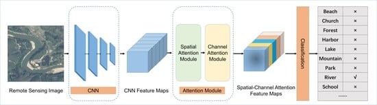
2.1. Overall Architecture

The overall architecture of our proposed method is shown in Figure 2. It consists of three parts: feature extraction, feature enhancement, and classification. In the feature extraction, D-CNN extracts the high-level features of the input remote sensing scene images. In the feature enhancement, the spatial information in the CNN feature maps is enhanced by the spatial attention enhancement mechanism; then, the channel information in the spatial attention feature maps is enhanced by the channel attention enhancement mechanism; finally, the spatial-channel attention feature maps are obtained. In the classification, the spatial-channel attention feature maps are classified.

2.2. Feature Extraction

Extracting the features of remote sensing images using CNN is an important step of remote sensing scene classification methods based on deep learning, and the quality of feature extraction directly affects the classification effect. The traditional CNN is limited by the shape of the convolution kernels and cannot adapt to remote sensing scenes with complex structure and spatial distribution. Generally, there are two methods to solve such a problem. One method is data augmentation, which constructs a dataset with sufficient transformation by enlarging, reducing, and rotating the original remote sensing images. The other method introduces other features, to make the feature more adaptive by adding scale-invariant features or rotation-invariant features. However, these two methods will bring a computational burden and make the classification algorithm complex.
By contrast, the deformable convolution [34] enhances its adaptability to complex remote sensing scenes by adding two offset parameters to the sampling position of the standard convolution. In this way, the sampling grid of the convolution can be shifted horizontally and vertically in the opposite direction. The comparison of standard convolution and deformable convolution is shown in Figure 3.
The standard convolution is calculated as follows:
y p i = p i R W p i · x p i
where p i is the position of the regular grid R on the input feature map x ; y is the output feature map, and W is the weight. After the offset, Δ p n is added to p i , p i + Δ p n represents a position of the feature map. The standard convolution is converted to deformable convolution as follows:
y p i = p i R W p i · x p i + Δ p n
The corresponding deformable pooling can be expressed as:
y p i = y p i n R
where n R is the number of regular grids.
Based on deformable convolution and deformable pooling, this study constructs D-CNN, and the framework is shown in Table 1. D-CNN is composed of a deformable convolution layer, a deformable pooling layer, and four deformable convolution blocks, × n means the stack block is repeated n times. Specifically, the first layer is a deformable convolution layer with a convolution filter size of 7 × 7, and the number of convolution filters is 64. The feature is first extracted extensively by a larger size deformable convolution, and the information of the original image is preserved as much as possible, so that the feature can be extracted in detail by the deformable convolution blocks later. The second layer is a deformable pooling layer with a pooling filter size of 3 × 3. The third layer consists of three deformable convolution block 1. In deformable convolution block 1, 64 1 × 1 convolution, 64 3 × 3 deconvolution, and 256 1 × 1 convolution are stacked sequentially. Each block is connected internally through a shortcut connection to avoid network degradation caused by the increase of network depth. Other deformable convolution blocks are similar to deformable convolution block 1. In the deformable convolution block, stacking multiple 3 × 3 deformable convolutions can increase the number of sampling locations and improve the expressiveness of the feature with a significant reduction in the number of parameters. For example, comparing 3 stacked 3 × 3 deformable convolutions with 1 7 × 7 deformable convolution: (1) the number of sampling positions for 3 stacked 3 × 3 deformable convolutions are (3 × 3)3 = 729, while the number of sampling positions for 1 7 × 7 deformable convolution are 7 × 7 = 49; (2) the number of parameters for 3 stacked 3 × 3 deformable convolutions are 3 × 3 × 3 × Cout × Cin = 27 Cout Cin, while the number of parameters for 1 7 × 7 deformable convolutions are 7 × 7× Cout × Cin = 49 Cout Cin, where C o u t and C i n represent the number of channels of output and input, respectively; (3) 3 stacked 3 × 3 deformable convolutions have 2 more activation functions than 1 7 × 7 deformable convolution.
As shown in Figure 4, by combining multiple deformable convolutions, the function of deformable convolution will be greatly improved. The small squares indicate the sampling points of the network, and the red arrow indicates the corresponding relationship between the feature maps of the two adjacent layers. From left to right, the feature maps are presented from low to high. The filter size of each layer is 3 × 3. The highlighted positions correspond to the highlighted units on the previous layer. It can be seen that the sampling position of the standard CNN is fixed for the object, while the deformable CNN can adapt to the shape of the object. The sampling point of the deformable CNN has a higher correlation with the object, which enhances the feature extraction of remote sensing scenes with complex structure and diverse distribution.

2.3. Feature Enhancement

Feature enhancement with attention mechanisms is a common and effective approach to improve deep learning methods. The attention mechanism in deep learning is similar to the human selective visual attention mechanism, which aims to select critical information from a multitude of information. In this study, SCA is proposed for remote sensing scenes. Spatial attention information and channel attention information are extracted by spatial attention module and channel attention module, respectively. Based on this, comprehensive attention information can be obtained.

2.3.1. Spatial Attention Module

The spatial attention module extracts the relationship between the spatial locations of the feature maps, as shown in Figure 5. Suppose the input feature maps P C × H × W , where C , H , and W represent the channel, height, and width of the feature maps, respectively. First, P is converted to A , B , D C × H × W by a convolution operation, and A and B are reshaped to C × N , where N = H × W . Then, matrix multiplication is performed between A and the transpose of B, and the spatial attention matrix S H × W × H × W is obtained by softmax:
s j i = exp A i · B j i = 1 N exp A i · B j
where s i j denotes the influence of position i on position j . The more similar the features of two locations, the greater the correlation between them. After this, the spatial attention matrix is multiplied with the feature map D to obtain the spatial location-enhanced feature map F s :
F s = i = 1 N s j i D i

2.3.2. Channel Attention Module

The channel attention module extracts the relationship between the individual channels of the feature maps, as shown in Figure 6. Unlike the spatial attention module, matrix multiplication is performed directly between P and the transpose of P, and the channel attention matrix X C × C is obtained by softmax:
x j i = exp P i · P j i = 1 N exp P i · P j
where x j i denotes the influence of channel i on channel j . After this, the channel attention matrix is multiplied with the feature map P to obtain the feature map F c for channel position enhancement:
F c = i = 1 C x j i P i

2.4. Classification

In the classification, global average pooling is employed to reduce the dimension of the global average of F from C × H × W to C × 1 × 1 , which greatly reduces the number of parameters. Then, the softmax function is used to achieve the final scene classification:
L = 1 N n = 1 N c = 1 C l o g exp θ c x n i = 1 C exp θ i x n ,   y n = c 0 , y n c
where x is the result of feature concatenation; y is the scene label; θ is the classifier parameter; C is the number of scene categories, and N is the number of training samples.

3. Experiment and Analysis

3.1. Datasets

To evaluate the effectiveness of the proposed method on remote sensing scenes, experiments are conducted on three remote sensing scene image datasets, and the comparison of the three datasets is shown in Table 2.
(1)
UCM: UC Merced Land Use dataset [16] was constructed by Yang et al. of the University of California at Merced using the United States Geological Survey National Map. The dataset contains 21 land use classes, with 100 samples in each class and a total of 2100 images. The size of each image is 256 × 256, with a spatial resolution of 0.3 m per pixel. Some samples from the UCM dataset are shown in Figure 7. UCM is an early proposed remote sensing scene dataset, and it is also one of the most widely used datasets.
(2)
NWPU: NWPU-RESISC45 dataset [35] was built by Cheng et al. of Northwestern Polytechnical University using Google Earth. The dataset contains 45 scenes, with 700 samples in each class and a total of 31,500 images. The size of each image is 256 × 256, with a spatial resolution of 0.2–30 m per pixel. Some samples from the NWPU Dataset are shown in Figure 8. NWPU is the remote sensing scene dataset with the richest scene categories and the largest number of samples so far. Besides, there are great variations in translation, spatial resolution, viewpoint, object pose, illumination, background, and occlusion, which makes it difficult for remote sensing scene classification.
(3)
AID: Aerial Image dataset [36] was built by Xia et al. of Wuhan University using Google Earth. The dataset contains 30 scenes, with 200−400 samples in each class and a total of 10,000 images. The size of each image is 600 × 600, with a spatial resolution of 0.5−8 m per pixel. Some samples from the AID Dataset are shown in Figure 9. Among the current remote sensing scene datasets, AID has the largest image size, which provides richer information for scene classification.

3.2. Evaluating Indexes

Overall accuracy (OA) and confusion matrix (CM) are used as evaluation indexes for remote sensing scene classification.
(1)
OA: It is defined as the proportion of the number of correctly classified samples to the total number of samples in the test set. It simply and effectively represents the prediction capacity of the model on the overall dataset. OA is calculated as follows:
OA = 1 T i m j n I f x i , j = y i , j
where T is the total number of samples in the test set; m and n are the total number of categories and the number of samples of each category, respectively; f ( ) is a classification function that predicts the category of a single sample x in the test set; y is the sample label indicating the real category of the sample; I ( ) is the indicator function, which takes the value of 1 when it is true and 0 when it is false.
(2)
CM: It uses a matrix of N rows and N columns to represent the classification effect, where each row represents the actual category and each column represents the predicted value. It can indicate the categories that are prone to confusion, thus more intuitively representing the performance of the algorithm.

3.3. Implementation Details

The experiments are conducted on an AI Studio platform equipped with Tesla V100 (32GB memory). The initial learning rate is 0.01. Every 20 epochs, the learning rate is divided by 10. Besides, the momentum is set to 0.9.

3.4. The Performance of the Proposed Method

3.4.1. Results on UCM

To demonstrate the superiority of our proposed method, it is compared with other methods on UCM, including Bidirectional adaptive feature fusion method (BDFF method) [25], Multiscale CNN (MCNN) [37], ResNet with weighted spatial pyramid matching collaborative representation-based classification (ResNet with WSPM-CRC) [38], VGG16 with multi-layer stacked covariance pooling (VGG16 with MSCP) [26], Gated bidirectional network (GBNet) [29], Feature aggregation CNN (FACNN) [39], Scale-free CNN (SF-CNN) [40], Deep discriminative representation learning with attention map method (DDRL-AM method) [41], and CNN based on attention-oriented multi-branch feature fusion (AMB-CNN) [42]. The training ratio of 80% is used on this dataset, and OA is taken as the evaluation index. The results are shown in Figure 10. Our method achieves the best OA of up to 99.62%.
Then, CM is adopted to analyze the performance of our proposed method in detail, and the results are shown in Figure 11. The vast majority of results are correct. The error only occurs between confusing categories such as dense residential, medium residential, and mobile home park, while the classification results of other categories are correct.
The above experiments show that our method achieves good performance on UCM, which is a dataset with a small sample type and sample size.

3.4.2. Results on NWPU

Compared with UCM, NWPU has 45 scene classes and 700 images per class. Therefore, NWPU can better reflect the performance of scene classification methods. On NWPU, our proposed method is compared with other methods, including CNN-CapsNet [43], Discriminative CNN with VGG16 (D-CNN with VGG16) [44], VGG16 with MSCP [26], Skip-connected covariance network (SCCov Network) [45], and AMB-CNN [42]. The training ratios of 10% and 20% are used on this dataset, respectively, and the results are shown in Figure 12. Regardless of the training ratio, our method achieves the best classification accuracy.
Then, CM is adopted to analyze the performance of our proposed method in detail, and the results are shown in Figure 13 and Figure 14. Our method achieves a good classification accuracy on each scene. When the training ratio is 10%, it achieves an OA of more than 90% on 26 of the 45 scenes and 80% on 44 scenes. When the training ratio is 20%, it achieves an OA of more than 90% on 43 of the 45 scenes and 100% on 9 scenes.
The above experiments show that our method still achieves a good classification accuracy under a large scene type and size.

3.4.3. Results on AID

Different from UCM and NWPU, the image size in AID reaches 600 × 600. To test the classification performance of our proposed method for large-scale remote sensing images, it is compared with other methods on AID, including CNN-CapsNet [43], D-CNN with VGG16 [44], VGG16 with MSCP [26], GBNet [29], SCCov Network [45], and AMB-CNN [42]. The training ratios of 20% and 50% are used on this dataset, respectively, and the results are shown in Figure 15. When the training ratio is 20%, our method achieves the best classification accuracy. When the training ratio is 50%, the difference between our method and the best classification method is 0.45%.
Then, CM is adopted to analyze the performance of our proposed method in detail, and the results are shown in Figure 16 and Figure 17. Our method achieves a good classification accuracy on each scene. When the training ratio is 20%, it achieves an OA of more than 90% on 24 of the 30 scenes, and more than 80% on all scenes, and even 100% on 9 scenes. When the training ratio is 50%, it achieves an OA of more than 90% on all scenes and even 100% for 12 scenes.

4. Discussion

4.1. Analysis of D-CNN

In Section 2.2, the principle of D-CNN is described in detail. In the experiment, more tests are conducted to show the effectiveness of D-CNN. The test results are shown in Figure 18, the yellow point indicates the activation unit and the red point indicates the sampling location. In D-CNN, three deformable convolutional layers are stacked, and the size of the deformable filters in each layer is 3 × 3. Therefore, each active unit corresponds to (3 × 3)3 = 729 sampling locations. It clearly shows that: if the activate unit is in the green space, the sampling locations are adjusted to the shape of the green space; if the activate unit is in the basketball court, the sampling locations are adjusted to the shape of the basketball court; if the activate unit is in the island, the sampling locations are adjusted to the shape of the island; if the activate unit is in the sea, the sampling locations are adjusted to the shape of the sea. The sampling locations are adaptively adjusted to the shape of objects in D-CNN.

4.2. Analysis of SCA

To evaluate the feature enhancement ability of SCA, SCA is added to other classical CNNs, and experiments are conducted on the AID dataset; 20% of the data in the AID dataset is randomly selected for training and the remaining data is used for testing. Meanwhile, OA is taken as the evaluation index. The experimental results are shown in Figure 19. It can be seen that SCA is applicable to a variety of classic CNNs and improves the classification accuracy. Especially for GoogLeNet, the classification accuracy is improved by 5.35%.
As each attention module has different functions, the arrangement strategies of attention modules affect the overall performance. Table 3 summarizes the experimental results on different attention arranging methods. Note that the spatial attention module outperforms using the channel attention module. In addition, the spatial-channel attention module performs better than the channel-spatial module. This is because the deformable convolution in D-CNN changes the sampling positions of the convolution kernel. Additionally, the feature maps have discriminative spatial features, which is conducive to the spatial attention module to enhance the spatial features. Moreover, the channel attention module associates scene types with the channels of the feature maps, which enhances the effectiveness of the overall approach. Reasonable attention module arrangement strategy improves the classification accuracy.

4.3. Visualization

In addition to using specific indices to evaluate the performance of the proposed method, this study also uses Gradient-weighted Class Activation Mapping (Grad-CAM) [45] to visualize the proposed method to analyze the concerns of the model. The results are shown in Figure 20. Grad-CAM reflects the distribution of the sensitive area of the proposed method to the scenes through heat map. The more contribution to the classification results, the redder the color on the heat map. It is obvious that our method focuses well on differentiated positions.

5. Conclusions

The complex shape and diverse distribution of remote sensing scenes bring challenges to remote sensing scene classification. To address this problem, this paper proposed a new feature extraction network called D-CNN and a new feature enhancement method called SCA. D-CNN uses deformable convolution to change the convolution sampling position. Based on this, the applicability of the network to irregular remote sensing scene images and the feature extraction capability is improved. As for SCA, it first extracts spatial key information and then extracts key channels to enhance effective features while suppressing invalid features. Extensive experiments have been conducted on three data (UCM, NWPU, and AID). The experimental results indicate that our method achieves good classification performance under various scene types and sizes and training ratios.

Author Contributions

D.W. and J.L. contributed equally to the study and are co-first authors. All authors have read and agreed to the published version of the manuscript.

Funding

This research was funded by the Advance Research Program (61403110404), the Advance Research Program (41416040203), and the Scientific and Technological Innovation Foundation of Shunde Graduate School, USTB (BK19CE019).

Institutional Review Board Statement

Not applicable.

Informed Consent Statement

Not applicable.

Data Availability Statement

The UC Merced Land Use Dataset in this study are openly and freely available at http://weegee.vision.ucmerced.edu/datasets/landuse.html (accessed on 9 December 2021). The NWPU-RESISC45 Dataset in this study are openly and freely available at http://www.escience.cn/people/JunweiHan/NWPU-RESISC45.html (accessed on 9 December 2021). The Aerial Image Dataset in this study are openly and freely available at http://www.captain-whu.com/project/AID/ (accessed on 9 December 2021).

Acknowledgments

We would like to thank the editor and reviewers for their reviews which improved the content of this paper.

Conflicts of Interest

The authors declare no conflict of interest.

References

  1. Qi, K.; Wu, H.; Shen, C.; Gong, J. Land-use scene classification in high-resolution remote sensing images using improved correlatons. IEEE Geosci. Remote Sens. Lett. 2015, 12, 2403–2407. [Google Scholar]
  2. Weng, Q.; Mao, Z.; Lin, J.; Liao, X. Land-use scene classification based on a CNN using a constrained extreme learning machine. Int. J. Remote Sens. 2018, 39, 6281–6299. [Google Scholar] [CrossRef]
  3. Wu, H.; Liu, B.; Su, W.; Zhang, W.; Sun, J. Hierarchical coding vectors for scene level land-use classification. Remote Sens. 2016, 8, 436. [Google Scholar] [CrossRef] [Green Version]
  4. Zhang, D.; Pan, Y.; Zhang, J.; Hu, T.; Zhao, J.; Li, N.; Chen, Q. A generalized approach based on convolutional neural networks for large area cropland mapping at very high resolution. Remote Sens. Environ. 2020, 247, 111912. [Google Scholar] [CrossRef]
  5. Shi, S.; Chang, Y.; Wang, G.; Li, Z.; Hu, Y.; Liu, M.; Li, Y.; Li, B.; Zong, M.; Huang, W. Planning for the wetland restoration potential based on the viability of the seed bank and the land-use change trajectory in the Sanjiang Plain of China. Sci. Total Environ. 2020, 733, 139208. [Google Scholar] [CrossRef]
  6. Zheng, X.; Yuan, Y.; Lu, X. A deep scene representation for aerial scene classification. IEEE Trans. Geosci. Remote Sens. 2019, 57, 4799–4809. [Google Scholar] [CrossRef]
  7. Zhu, Q.; Zhong, Y.; Zhang, L.; Li, D. Adaptive deep sparse semantic modeling framework for high spatial resolution image scene classification. IEEE Trans. Geosci. Remote Sens. 2018, 56, 6180–6195. [Google Scholar] [CrossRef]
  8. Tayyebi, A.; Pijanowski, B.C.; Tayyebi, A.H. An urban growth boundary model using neural networks, GIS and radial parameterization: An application to Tehran, Iran. Landsc. Urban Plan. 2011, 100, 35–44. [Google Scholar] [CrossRef]
  9. Fingas, M.; Brown, C. Review of oil spill remote sensing. Mar. Pollut. Bull. 2014, 83, 9–23. [Google Scholar] [CrossRef] [Green Version]
  10. Yi, Y.; Zhang, Z.; Zhang, W.; Jia, H.; Zhang, J. Landslide susceptibility mapping using multiscale sampling strategy and convolutional neural network: A case study in Jiuzhaigou region. CATENA 2020, 195, 104851. [Google Scholar] [CrossRef]
  11. Gitas, I.; Polychronaki, A.; Katagis, T.; Mallinis, G. Contribution of remote sensing to disaster management activities: A case study of the large fires in the Peloponnese, Greece. Int. J. Remote Sens. 2008, 29, 1847–1853. [Google Scholar] [CrossRef]
  12. Risojević, V.; Babić, Z. Fusion of global and local descriptors for remote sensing image classification. IEEE Geosci. Remote Sens. Lett. 2013, 10, 836–840. [Google Scholar] [CrossRef]
  13. Ojala, T.; Pietikainen, M.; Maenpaa, T. Multiresolution gray-scale and rotation invariant texture classification with local binary patterns. IEEE Trans. Pattern Anal. Mach. Intell. 2002, 24, 971–987. [Google Scholar] [CrossRef]
  14. Lowe, D.G. Distinctive image features from scale-invariant keypoints. Int. J. Comput. Vis. 2004, 60, 91–110. [Google Scholar] [CrossRef]
  15. Dalal, N.; Triggs, B. Histograms of oriented gradients for human detection. In Proceedings of the IEEE Conference on Computer Vision and Pattern Recognition, San Diego, CA, USA, 20–26 June 2005; pp. 886–893. [Google Scholar]
  16. Yang, Y.; Newsam, S. Bag-of-visual-words and spatial extensions for land-use classification. In Proceedings of the International Conference on Advances in Geographic Information Systems, San Jose, CA, USA, 2–5 November 2010; pp. 270–279. [Google Scholar]
  17. Lazebnik, S.; Schmid, C.; Ponce, J. Beyond bags of features: Spatial pyramid matching for recognizing natural scene categories. In Proceedings of the IEEE Conference on Computer Vision and Pattern Recognition, New York, NY, USA, 17–22 June 2006; pp. 2169–2178. [Google Scholar]
  18. Perronnin, F.; Sánchez, J.; Mensink, T. Improving the fisher kernel for large-scale image classification. In Proceedings of the European Conference on Computer Vision, Heidelberg, Germany, 5 September 2010; pp. 143–156. [Google Scholar]
  19. Jégou, H.; Perronnin, F.; Douze, M.; Sánchez, J.; Pérez, P.; Schmid, C. Aggregating local image descriptors into compact codes. IEEE Trans. Pattern Anal. Mach. Intell. 2012, 34, 1704–1716. [Google Scholar] [CrossRef] [PubMed] [Green Version]
  20. Krizhevsky, A.; Sutskever, I.; Hinton, G.E. ImageNet classification with deep convolutional neural networks. In Proceedings of the International Conference on Neural Information Processing Systems, Tahoe, NV, USA, 3–6 December 2012; pp. 1097–1105. [Google Scholar]
  21. Simonyan, K.; Zisserman, A. Very deep convolutional networks for large-scale image recognition. arXiv 2014, arXiv:1409.1556. [Google Scholar]
  22. He, K.; Zhang, X.; Ren, S.; Sun, J. Deep residual learning for image recognition. In Proceedings of the IEEE Conference on Computer Vision and Pattern Recognition, Las Vegas, NV, USA, 27–30 June 2016; pp. 770–778. [Google Scholar]
  23. Huang, G.; Liu, Z.; Maaten, L.V.D.; Weinberger, K.Q. Densely connected convolutional networks. In Proceedings of the IEEE Conference on Computer Vision and Pattern Recognition, Honolulu, HI, USA, 21–26 July 2017; pp. 2261–2269. [Google Scholar]
  24. Li, E.; Xia, J.; Du, P.; Lin, C.; Samat, A. Integrating multilayer features of convolutional neural networks for remote sensing scene classification. IEEE Trans. Geosci. Remote Sens. 2017, 55, 5653–5665. [Google Scholar] [CrossRef]
  25. Lu, X.; Ji, W.; Li, X.; Zheng, X. Bidirectional adaptive feature fusion for remote sensing scene classification. Neurocomputing 2019, 328, 135–146. [Google Scholar] [CrossRef]
  26. He, N.; Fang, L.; Li, S.; Plaza, A.; Plaza, J. Remote sensing scene classification using multilayer stacked covariance pooling. IEEE Trans. Geosci. Remote. Sens. 2018, 56, 6899–6910. [Google Scholar] [CrossRef]
  27. Flores, E.; Zortea, M.; Scharcanski, J. Dictionaries of deep features for land-use scene classification of very high spatial resolution images. Pattern Recognit. 2019, 89, 32–44. [Google Scholar] [CrossRef]
  28. Fang, J.; Yuan, Y.; Lu, X.; Feng, Y. Robust space–frequency joint representation for remote sensing image scene classification. IEEE Trans. Geosci. Remote. Sens. 2019, 57, 7492–7502. [Google Scholar] [CrossRef]
  29. Sun, H.; Li, S.; Zheng, X.; Lu, X. Remote sensing scene classification by gated bidirectional network. IEEE Trans. Geosci. Remote. Sens. 2020, 58, 82–96. [Google Scholar] [CrossRef]
  30. Bi, Q.; Qin, K.; Li, Z.; Zhang, H.; Xu, K.; Xia, G.-S. A multiple-instance densely-connected ConvNet for aerial scene classification. IEEE Trans. Image Process. 2020, 29, 4911–4926. [Google Scholar] [CrossRef] [PubMed]
  31. Wu, X.; Zhang, Z.; Zhang, W.; Yi, Y.; Zhang, C.; Xu, Q. A convolutional neural network based on grouping structure for scene classification. Remote Sens. 2021, 13, 2457. [Google Scholar] [CrossRef]
  32. Xie, H.; Chen, Y.; Ghamisi, P. Remote sensing image scene classification via label augmentation and intra-class constraint. Remote Sens. 2021, 13, 2566. [Google Scholar] [CrossRef]
  33. Chen, J.; Huang, H.; Peng, J.; Zhu, J.; Chen, L.; Tao, C.; Li, H. Contextual information-preserved architecture learning for remote-sensing scene classification. IEEE Trans. Geosci. Remote Sens. 2021, 60, 5602614. [Google Scholar] [CrossRef]
  34. Dai, J.; Qi, H.; Xiong, Y.; Li, Y.; Zhang, G.; Hu, H.; Wei, Y. Deformable convolutional networks. In Proceedings of the IEEE International Conference on Computer Vision, Venice, Italy, 22–29 October 2017; pp. 764–773. [Google Scholar]
  35. Cheng, G.; Han, J.; Lu, X. Remote sensing image scene classification: Benchmark and state of the art. Proc. IEEE 2017, 105, 1865–1883. [Google Scholar] [CrossRef] [Green Version]
  36. Xia, G.; Hu, J.; Hu, F.; Shi, B.; Bai, X.; Zhong, Y.; Zhang, L.; Lu, X. AID: A benchmark data set for performance evaluation of aerial scene classification. IEEE Trans. Geosci. Remote Sens. 2017, 55, 3965–3981. [Google Scholar] [CrossRef] [Green Version]
  37. Liu, Y.; Zhong, Y.; Qin, Q. Scene classification based on multiscale convolutional neural network. IEEE Trans. Geosci. Remote. Sens. 2018, 56, 7109–7121. [Google Scholar] [CrossRef] [Green Version]
  38. Liu, B.-D.; Meng, J.; Xie, W.-Y.; Shao, S.; Li, Y.; Wang, Y. Weighted spatial pyramid matching collaborative representation for remote-sensing-image scene classification. Remote Sens. 2019, 11, 518. [Google Scholar] [CrossRef] [Green Version]
  39. Lu, X.; Sun, H.; Zheng, X. A feature aggregation convolutional neural network for remote sensing scene classification. IEEE Trans. Geosci. Remote Sens. 2019, 57, 7894–7906. [Google Scholar] [CrossRef]
  40. Xie, J.; He, N.; Fang, L.; Plaza, A. Scale-free convolutional neural network for remote sensing scene classification. IEEE Trans. Geosci. Remote Sens. 2019, 57, 6916–6928. [Google Scholar] [CrossRef]
  41. Li, J.; Lin, D.; Wang, Y.; Xu, G.; Zhang, Y.; Ding, C.; Zhou, Y. Deep discriminative representation learning with attention map for scene classification. Remote Sens. 2020, 12, 1366. [Google Scholar] [CrossRef]
  42. Shi, C.; Zhao, X.; Wang, L. A multi-branch feature fusion strategy based on an attention mechanism for remote sensing image scene classification. Remote Sens. 2021, 13, 1950. [Google Scholar] [CrossRef]
  43. Wei, Z.; Tang, P.; Zhao, L. Remote sensing image scene classification using CNN-CapsNet. Remote Sens. 2019, 11, 494. [Google Scholar]
  44. Cheng, G.; Yang, C.; Yao, X.; Guo, L.; Han, J. When deep learning meets metric learning: Remote sensing image scene classification via learning discriminative CNNs. IEEE Trans. Geosci. Remote Sens. 2018, 56, 2811–2821. [Google Scholar] [CrossRef]
  45. He, N.; Fang, L.; Li, S.; Plaza, J.; Plaza, A. Skip-connected covariance network for remote sensing scene classification. IEEE Trans. Neural Netw. Learn. Syst. 2020, 31, 1461–1474. [Google Scholar] [CrossRef] [Green Version]
Figure 1. Examples of remote sensing scene images. (a) Complex outline and structure; (b) Complex spatial distribution; (c) Intra-class diversity; (d) Inter-class similarity.
Remotesensing 13 05076 g001
Figure 2. The overall architecture of our proposed method.
Remotesensing 13 05076 g002
Figure 3. Illustration of the sampling locations in 3 × 3 standard and deformable convolution. (a) Regular sampling grid (blue squares) of standard convolution; (b) Deformed sampling location (yellow squares) with offsets in deformable convolution.
Remotesensing 13 05076 g003
Figure 4. Comparison of the sampling locations of standard CNN and deformable CNN. (a) The sampling position of the standard CNN is fixed; (b) The sampling position of the deformable CNN adapts to the shape of the object.
Remotesensing 13 05076 g004
Figure 5. Spatial attention module.
Remotesensing 13 05076 g005
Figure 6. Channel attention module.
Remotesensing 13 05076 g006
Figure 7. The UCM dataset.
Remotesensing 13 05076 g007
Figure 8. The NWPU dataset.
Remotesensing 13 05076 g008
Figure 9. The AID dataset.
Remotesensing 13 05076 g009
Figure 10. The OA (%) of different methods on UCM under the training ratio of 80%.
Remotesensing 13 05076 g010
Figure 11. CM on UCM under the training ratio of 80%.
Remotesensing 13 05076 g011
Figure 12. The OA (%) of different methods on NWPU under the training ratio of 10% and 20%.
Remotesensing 13 05076 g012
Figure 13. CM on NWPU under the training ratio of 10%.
Remotesensing 13 05076 g013
Figure 14. CM on NWPU under the training ratio of 20%.
Remotesensing 13 05076 g014
Figure 15. The OA (%) of different methods on AID under the training ratio of 20% and 50%.
Remotesensing 13 05076 g015
Figure 16. CM on AID under the training ratio of 20%.
Remotesensing 13 05076 g016
Figure 17. CM on AID under the training ratio of 50%.
Remotesensing 13 05076 g017
Figure 18. Sampling locations of the D-CNN. (a) Basketball court; (b) Island.
Remotesensing 13 05076 g018
Figure 19. CM on AID under the training ratio of 20%.
Remotesensing 13 05076 g019
Figure 20. Visualizations for scenes sampled from the NWPU dataset. The redder color indicates the higher classification contribution and the more blue color represents the lower classification contribution.
Remotesensing 13 05076 g020aRemotesensing 13 05076 g020b
Table 1. Framework of the proposed D-CNN.
Layer NameTypeFiltersSize
deformable convolutiondeformable convolution647 × 7
deformable poolingdeformable pooling 3 × 3
deformable convolution block 1convolution641 × 1× 3
deformable convolution643 × 3
convolution2561 × 1
deformable convolution block 2convolution1281 × 1× 4
deformable convolution1283 × 3
convolution5121 × 1
deformable convolution block 3convolution2561 × 1× 6
deformable convolution2563 × 3
convolution10241 × 1
deformable convolution block 4convolution5121 × 1× 3
deformable convolution5123 × 3
convolution20481 × 1
Table 2. The comparison of the three datasets.
DatasetsScene ClassesImages Per ClassTotal ImagesImage SizesSpatial Resolution
(in meters)
UCM211002100256 × 2560.3
NWPU4570031,500256 × 2560.2–30
AID30220−40010,000600 × 6000.5–8
Table 3. The comparison between different strategies.
MethodOA (%) under the Training Ratio of 20%OA (%) under the Training Ratio of 50%
D-CNN87.6288.35
D-CNN + spatial90.2892.23
D-CNN + channel89.6791.56
D-CNN + channel + spatial93.2894.26
D-CNN + spatial + channel94.6396.43
Publisher’s Note: MDPI stays neutral with regard to jurisdictional claims in published maps and institutional affiliations.

