Article

Multimodal Data and Multiscale Kernel-Based Multistream CNN for Fine Classification of a Complex Surface-Mined Area

1
School of Land Science and Technology, China University of Geosciences, Beijing 100083, China
2
Key Laboratory of Land Consolidation and Rehabilitation, Ministry of Natural Resources, Beijing 100035, China
3
School of Computer Science, China University of Geosciences, Wuhan 430074, China
4
Hubei Key Laboratory of Intelligent Geo-Information Processing, China University of Geosciences, Wuhan 430074, China
*
Author to whom correspondence should be addressed.
Remote Sens. 2021, 13(24), 5052; https://doi.org/10.3390/rs13245052
Submission received: 31 October 2021 / Revised: 4 December 2021 / Accepted: 9 December 2021 / Published: 13 December 2021

Abstract

:
Fine land cover classification (FLCC) of complex landscapes is a popular and challenging task in the remote sensing community. In complex surface-mined areas (CSMAs), researchers have conducted FLCC using traditional machine learning methods and deep learning algorithms. However, convolutional neural network (CNN) algorithms that may be useful for FLCC of CSMAs have not been fully investigated. This study proposes a multimodal remote sensing data and multiscale kernel-based multistream CNN (3M-CNN) model. Experiments based on two ZiYuan-3 (ZY-3) satellite imageries of different times and seasons were conducted in Wuhan, China. The 3M-CNN model had three main features: (1) multimodal data-based multistream CNNs, i.e., using ZY-3 imagery-derived true color, false color, and digital elevation model data to form three CNNs; (2) multisize neighbors, i.e., using different neighbors of optical and topographic data as inputs; and (3) multiscale convolution flows revised from an inception module for optical and topographic data. Results showed that the proposed 3M-CNN model achieved excellent overall accuracies on two different images, and outperformed other comparative models. In particular, the 3M-CNN model yielded obvious better visual performances. In general, the proposed process was beneficial for the FLCC of complex landscape areas.

1. Introduction

Land cover classification (LCC) [1,2] is one of the most popular topics in the remote sensing community. With the enhancement of the spatial resolution of remote sensing imagery, fine LCC (FLCC) [3,4,5,6,7] of complex landscapes has attracted increasing attention because of the need to improve accuracy. Owing to the complex features of three-dimensional terrain, FLCC of complex surface-mined areas (CSMAs) is challenging and of great importance for mine development.
The solution of FLCC applied to CSMAs involves the use of multimodal data for feature learning and advanced algorithms for classification [8,9]. Firstly, feature engineering coupled with machine learning algorithms (MLAs) is effective. Feature engineering mainly includes hand-crafted feature calculation, feature selection (FS), and feature extraction (i.e., feature reduction). FS uses an algorithm to choose a representative feature combination. Feature extraction uses algorithms [10] to extract a combination of new features. For example, Azeez et al. [11] used support vector machine (SVM), decision tree (DT), and random forest (RF) algorithms for LCC of a regional agricultural area. Our previous studies have used this scheme. For example, Li et al. [12] proposed a fine classification framework for three surface-mined land cover classes using multimodal spatial, spectral, and topographic features from ZiYuan-3 (ZY-3) imagery. Additionally, an FS method and RF, SVM, and artificial neural network (ANN) algorithms were used. For FLCC of CSMAs, Chen et al. [13] assessed the importance of feature sets based on an FS method; Chen et al. [14] utilized multiple features derived from WorldView-3 imagery and some optimized SVM models. In addition, Chen et al. [8] conducted a review of FLCC in CSMAs using remote sensing data. The shortcoming of each of the above-mentioned methods was that the feature sets derived by feature engineering were insufficient for representation.
Deep learning (DL) algorithms have been widely used in computer vision and remote sensing fields because they can learn informative high-level features. As a result, some researchers have examined many DL algorithm-based schemes for LCC and FLCC. For example, Lv et al. [15] used a deep belief network (DBN)-based method for LCC. Li et al. [16] utilized a stacked autoencoder (SAE) method for LCC, while Tong et al. [17] proposed a transferable convolutional neural network (CNN) model for LCC. For FLCC of CSMAs, Li et al. [9] proposed a multimodal and multimodel deep fusion strategy based on ZY-3 imagery, the DBN algorithm, and two MLAs (i.e., RF and SVM). Li et al. [18] proposed a novel multi-level, output-based DBN. Compared to SAE and DBN, CNN has stronger representation ability due to the consideration of spatial neighborhood information, which has seldom been examined for FLCC.
In addition to directly using DL algorithms, some researchers have explored multistream CNNs based on multiple inputs. For example, Liu et al. [19] applied a triplet CNN for remote sensing scene classification. Others were based on multimodal data such as hyperspectral image (HSI) and light detection and ranging (LiDAR) data. For example, Li et al. [20] proposed a three-stream CNN model based on the spectral and spatial features of HSI and the topographic features of LiDAR data. Xu et al. [21] developed a two-branch CNN based on HSI and LiDAR data. Moreover, a two-tunnel CNN framework was first used to extract deep spectral-spatial features of HSI. Chen et al. [22] proposed a similar two-stream CNN based on HSI and LiDAR data. Chen et al. [23] utilized multispectral (MS) image/HSI and LiDAR to form a two-stream CNN. Jahan et al. [24] proposed a three-stream CNN using HSI and LiDAR data with a feature-reduction technique for LCC. Lastly, Rasti et al. [25] proposed a three-stream CNN using HSI and LiDAR data for LCC. Moreover, different band combinations that have been used as inputs of the DL algorithms have been considered worthy of investigation [26,27]. It has been suggested that the fusion methods for panchromatic (PAN) and MS images might affect the classification results [28,29,30].
Some researchers have focused on extracting multiscale features. For example, Zhang et al. [31] proposed a multiscale and multifeature-based CNN for LCC. Zhang et al. [32] proposed a multiscale dense network for LCC. They stated that the models with multi-scale features effectively improved classification accuracy.
Four influencing factors were pertinent to land cover classification over the study area: (1) Sample acquisition cost is high, as a result, a small sample classification situation was necessary; (2) There were complex features of the three-dimensional terrain, as a result topographic data was needed. How to effectively mine the multimodal multispectral image and topographic data was, therefore, an issue; (3) The topographic data were of lower spatial resolution than the multispectral images. This raised the question of how to fuse them; (4) The ground objects were at different scales. This raised the question of how to represent them.
Considering these influencing factors, the pipeline design was based on certain prior knowledge, reducing the need for sample data, as follows: (1) True color and false color images have different and complementary feature representation capabilities and can essentially replace multispectral data with four bands. Compared with using multi-spectral data as input, the spectral band combination method can reduce the demand for sample data; (2) The use of multi-branch extraction and post-fusion methods can avoid the interactions of different modal data due to different numerical units, meanings, and magnitudes, and theoretically is more conducive to the extraction of multimodal deep features; (3) Using multisize neighbors as inputs for data with different spatial resolutions can fully express the spatial relationship among different land covers; (4) In view of the multiscale characteristics of the ground objects, a multiscale convolution module was designed to ensure that the algorithms had multiscale feature extraction capabilities.
In this study, a novel multimodal remote data sensing, and multiscale kernel-based multistream CNN (3M-CNN), model was proposed for FLCC of CSMAs. The 3M-CNN model was tested using two ZY-3 imageries. The contributions to development of the approach were as follows:
(1)
We proposed a multimodal data-based multistream CNN model, which can extract multiple features from true color and false color images, and a digital elevation model (DEM) data that is derived from ZY-3 imagery.
(2)
We used multisize neighbors as the inputs of the CNN, i.e., using different neighbors for optical images and DEM data.
(3)
Multiscale convolution flows revised from the inception module were applied to optical images and DEM data, which could match different input neighbors.

2. Study Area and Data Source

As in our previous studies, we conducted experiments in Wuhan City, China in an area of 109.4 km2 [9,12,13] (Figure 1). The terrain of the study area is complex and includes multiple agricultural-related land covers in different phenological periods.
We first obtained four images from different cameras of the ZY-3 satellite on 20 June 2012 (Table 1). The processing of the four images resulted in two kinds of data. One was a 10 m DEM using a process of stereo image pairs of two 3.6 m front- and backward-facing PAN images. Using a process of pixel-level image fusion operation (i.e., Gram–Schmidt spectral sharpening), the other obtained image was a 2.1 m fused MS image based on the 2.1 m PAN and the 5.8 m MS images. To match the resolution of these two sets of data, the DEM was re-sampled to 2.1 m. The DEM included relative elevation data ranging from −14 m to 122 m.
Another scene of ZY-3 imagery on 11 November 2020 was obtained, preprocessed, and tested in this study (Figure 2). A 2.1 m fused MS image and a 2.1 m DEM data (resampled from 10 m) were also obtained. The DEM included relative elevation data with a range from −25 m to 113 m. Although the values of these two DEMs had some differences, these had little effect on the subsequent classification results, as they were first scaled before inputting to the classification models. These two sets of imageries, for different years and seasons, helped to evaluate the generalization capability of the proposed model.
Figure 3 shows a comparison of a sub-area from the two images. The red ellipses indicate the places with large changes. From Figure 3, we can see that the open-pit mining was growing rapidly.

3. Methods

In this section, the details of the 3M-CNN model are presented (Figure 4). The 3M-CNN model was influenced by: (1) the size of ground objects, which varied greatly; (2) data from different models that can show different characteristics of ground objects; and (3) a multiscale convolution kernel that can extract informative features. By combining these three concepts, a novel 3M-CNN method was proposed for FLCC of CSMAs. The FLCC scheme, various data sets, model development, and accuracy assessment are described below.

3.1. 3M-CNN Model

3.1.1. Multimodal Data-Based MultiStream CNN

MS data included 4 bands: red, green, blue, and near-infrared. To make full use of the MS image, we used the true color (i.e., R—red, G—green, B—blue), and false color (i.e., R—near-infrared, G—red, B—green) images as inputs, which had different representative ability. The false color image can help to distinguish between water and vegetation, which showed different red colors. Finally, based on two optical images and DEM data, a three-stream CNN was constructed.

3.1.2. Multisize Neighbors

It is worth noting that the DEM data were derived by interpolation, which resulted in more correlated pixels in the data. In other words, the same-size pixel neighbors from DEM and MS data failed to provide the same amount of valid classification information. Hence, we designed a series of experiments to calculate the best size of DEM data (i.e., N2 × N2 in Figure 4). In contrast, to simplify the procedure of parameter selection, the input size of MS (i.e., N1 × N1 in Figure 4) was fixed at 15 pixels × 15 pixels. Figure 5 and Figure 6 show the demonstration area (i.e., the input image in Figure 4) and subset areas for explaining the utilization of the 15 pixels × 15 pixels neighbor. From the subset areas of 1 to 5 and 7 to 8, we can see that the 15 pixels × 15 pixels neighbor can represent both the features of some land covers and their surrounding classes. Furthermore, from the subset area of 6, we can see that the 15 pixels × 15 pixels neighbors of some sample points in the data polygon (for details, see Section 3.3) covered some other sample points. This may have contributed to test accuracy and affected the parameter selection that was based on training and validation sets. We determined that the influences of the 15 pixels × 15 pixels neighbor were acceptable. Larger neighbors that may have larger negative impacts were not used.

3.1.3. Multiscale Convolutional Modules

The multiscale convolutional modules were revised from the inception block. To be specific, we used a parameter k, to magnify the kernel sizes.
To fully utilize the contextual information, two different strategies were pursued for DEM and other data. The branches of the true color and the false color data were designed with fixed convolutional kernels. As shown in Figure 7, the kernel sizes were always 1 × 1 + 3 × 3, 3 × 3 + 3 × 3, and 3 × 3 + 5 × 5. The branch of the DEM data was designed with varied kernels to match the input size. As shown in Figure 8, the kernel sizes of DEM data were k × k + 3k × 3k, 3k × 3k + 3k × 3k, and 3k × 3k + 5k × 5k. Hence, the parameter k could be objectively selected using training and validation sets.

3.2. FLCC Scheme

This study was committed to the FLCC of CMALs. To maintain continuity of research, the second-level LCC scheme described in Li et al. [9] was applied. It contained the following four types of croplands: paddy, greenhouse, green dry land, and fallow land; four types of forest lands: woodland, shrubbery, coerced forest, and nursery; two water classes: pond and stream (natural) and mine pit pond; three road classes: dark road, bright road, and light gray road; three types of residential lands: bright roof, red roof, and blue roof; one bare surface land; and three types of surface-mined land: open pit, ore processing site, and dumping ground.
All other operations, such as the division of the training set, validation set, and test set, parameter selection, and accuracy assessment, were conducted using the FLCC scheme. The two scenes of imageries have the same FLCC scheme.

3.3. Training, Validation and Test Set

First, some polygons in the study area were labeled manually. Then, sampling points were randomly selected for training, validation, and test sets according to the ratio 4:1:1 (see Figure 9). Subsequently, 2000, 500, and 500 samples of each class for the training set, validation set, and test set, respectively, were obtained. Finally, the experimental data sets contained five groups of training, validation, and test sets. More detail of the data sets can be found in Table 2. Similarly, for the imagery on 11 November 2020, the training, validation, and test sets with 2000, 500, and 500 random samples, respectively, for each land cover were also constructed.

3.4. Model Construction, Parameter Selection, and Model Comparison

The model structures and hyper-parameters from the imagery on 20 June 2012 were directly used for that on 11 November 2020.

3.4.1. Model Construction

As mentioned above, the 3M-CNN model had three different inputs. Each stream was constructed by two convolution flows, a flattened layer, a concatenating layer, and a fully connected layer. Then the three streams were concatenated. The output was subsequently placed into two fully connected layers. Finally, the result was produced.

3.4.2. Grid Search for Parameter Selection

Several parameters can affect the performance of a CNN, such as input size, kernel size, batch size, the iteration number (epoch), steps per epoch, learning rate, loss function, the activation function, and dropout. The first two were the most important parameters as well as the most difficult ones to select.
In general, the complex model might yield better performance. However, the complex model increased training difficulty and training time. Moreover, in the field of remote sensing, limited by the scarcity of labeled data, complex models often lead to serious underfitting issues.
In this study, the two above-mentioned parameters were selected. To simplify the parameter selection process, we fixed other parameters with different empirical values.
To determine the best parameters, we conducted two types of experiments.
Experiment 1: Input Size Selection. This experiment was used to find out the optimal input size of DEM data (i.e., N2 × N2) using the single-scale CNN model (Figure 10). The single-scale convolution flow is depicted in Figure 11, which contains two groups of convolution block, batch normalization (i.e., BN), the activation function (i.e., ReLU), and the maximum pooling layer. After the flattening and concatenation operations, two fully connected layers were applied. Then the Softmax classifier function was applied. The optimal input size was applied to the other experiments.
Experiment 2: Kernel Size Selection. This experiment utilized the optimal input size obtained in Experiment 1. Kernel size also required to be considered. As mentioned above, we designed different parameter values of k to find out the optimal kernel size for the 3M-CNN model.

3.4.3. Model Comparison

Firstly, by using the selected input size of DEM data, the single-scale CNN (Figure 10), and the 3M-CNN model, based on a multiscale kernel with k = 1, were compared with the final 3M-CNN-Magnify model, which was based on the multiscale kernel with the selected parameter value of k (Table 3). Then, the MLAs and DBN-based models in [9] were also compared.

3.5. Accuracy Assessment

The training and validation sets were used for model training and parameter selection, while the test set was used to conduct the quantitative evaluation.
The classification performances of the models were evaluated based on the average overall accuracy (OA), used time, quantity disagreement (QD), and allocation disagreement (AD) [33]. With respect to the results derived by ZiYuan-3 imagery on 20 June 2012, some former results in [9] were used for comparison. Visual assessment of the predicted maps was also conducted.

4. Results

4.1. Parameter Selection Results

4.1.1. Experiment 1: Input Size Selection

For this experiment, as shown in Figure 12, a series of input sizes ranging from 31 to 71, in intervals of 10, were applied. Five experiments were repeated. Training time was at a minimum value for an input size of 51, and the OA, at an input size of 51, exceeded that of the OAs of input sizes 31, 41, and 61. Although input size 71 resulted in a higher OA than that of input size 51, the training time for input size 71 was almost twice that of input size 51. Hence, we considered input size 51 to be optimal. The single-scale CNN with a size of 15 for spectral data and 51 for DEM achieved an average OA of 94.60%. This experiment indicated that input size magnification for single-scale CNN improved accuracy.

4.1.2. Experiment 2: Kernel Size Selection

For this experiment, we used 51 as the input size of DEM and 15 as the input size of the spectral data. The values of k were set from 1 to 4, in which 1 represented the original model, while 2, 3, and 4 represented the magnifying models. Specifically, we limited the value of k to a maximum of 4 because a larger kernel size caused small feature maps. If the value of k was set to 5, the feature maps in the middle of the model would be smaller than the kernel size, which would lead to model construction failure. Each value of k was applied to five random tests. As shown in Figure 13, when the k-value was set to 3, the model achieved the highest OA and took the least amount of time. It is of note that 51 divided by 15 is 3.4 which is greater than 3 and less than 4, and closer to 3. Therefore, from this point of view, a k-value of 3 was also most suitable for the model.

4.2. Precision Evaluation Result

After the parameter selection stage, the optimal models were obtained. Table 4 presents the OA, training time, QD, and AD values of the single-scale CNN, 3M-CNN, and 3M-CNN-Magnify models, and the models in [9]. The 3M-CNN-Magnify model achieved the highest OA value of 95.09% ± 0.29% and lowest AD value of 1.84% ± 0.22%. DBN took the least amount of training time. It was apparent that the more complex the model, the more computations were involved, which resulted in longer running times. Furthermore, multiple convolution layers based on feature maps needed more time than the coding layers of DBN based on feature vectors. Next, the model compression method to simplify the model and improve the running speed was considered.
Table 5 presents the OA, QD, and AD values for imagery on 11 November 2020. The 3M-CNN-magnify model achieved the highest OA value of 96.60% ± 0.22%, and lowest QD and AD values of 0.91% ± 0.13% and 2.47% ± 0.15%. The 3M-CNN-Magnify and 3M-CNN models outperformed the single-scale CNN model, with average OA improvements of 3.03% and 1.44%.

4.3. Visual Assessment of the Predicted Maps

To qualitatively evaluate the results, two predicted maps of the study area were produced. One was a map with 20 classes for FLCC, as depicted in Figure 14 (the bottom image). The other was a map with 7 classes for LCC as depicted in Figure 15 (the bottom image), which was derived from the FLCC map by grouping different second-level land covers into their corresponding first-level land covers.
Overall, the two maps were visually accurate. Compared to those derived from the DBN-SVM model in [9] (the upper images in Figure 14 and Figure 15), this study achieved better map results. For example, the bare surface land, residential land, dumping ground, green dry land, ore processing site, and pond and stream (i.e., the areas from 1 to 6 in Figure 14) in this study were classified more accurately. The Jing-zhu expressway (see Figure 1) was obviously misclassified by the DBN-SVM model. The bare surface land, residential land, and road (i.e., the areas 1, 3, and 4 in Figure 15) that were derived by the proposed model in this study were obviously better than those obtained by DBN-SVM. In particular, almost all the north-south roads were wrongly classified using the DBN-SVM model. There were also some misclassifications for the 7-class map by the proposed model in this study. For example, some crop lands were classified erroneously as forest lands at the right middle corner of the bottom map in Figure 15 (i.e., the area of 2).
Figure 16 shows the predicted maps of FLCC and LCC based on the 3M-CNN-Magnify model and ZY-3 imagery on 11 November 2020. These two predicted maps were both obtained based on the 3M-CNN-Magnify model.
Overall, the two maps in Figure 16 were visually accurate. There were three main differences between the maps of FLCC in Figure 14 and Figure 16: (1) there were more fallow lands in Figure 16, especially at the upper right corner; (2) there were more green dry lands in Figure 14. These two differences could be attributed to the seasons of the two images (one was in summer and the other in autumn); (3) there were some misclassifications in Figure 16. For example, many croplands at the bottom left corner (the area of 2) were classified as nursery. The dumping ground, crop land, and residential land (i.e., the areas 1, 3, and 4 in Figure 16) that were derived by the imagery on 11 November 2020 were better than those obtained on 20 June 2012.
The maps of LCC in Figure 15 and Figure 16 were similar overall. This result indicated that from 2012 to 2020, the changes among the first-level land covers were small.
In sum, from 2012 to 2020 there were basically no changes in the agricultural development pattern; however, open-pit mining grew rapidly.

5. Discussions

5.1. Effectiveness of Multimodal Data-Based Multistream CNN Structure

Figure 17 shows a diagram of the proposed scheme. When there were some land covers leading to terrain changes, topographic data were helpful for classification. At this time, the proposed model might be positive. We think this model is also suitable for other sensors, as follows: (1) When the other sensors have multi-view cameras (e.g., GaoFen-7 satellite), topographic data can be extracted directly. Then, this model is suitable; (2) When the other sensors can obtain only multispectral images, this model is also suitable because we can use some other topographic data. For example, data with lower resolution, such as advanced spaceborne thermal emission and reflection radiometer global digital elevation models, can be used, if their spatial resolution can describe the terrain changes of the study areas. Other topographic data with higher resolution can also be used, such as light detection and ranging data.
We can also replace DEM data with synthetic aperture radar (SAR), hyperspectral, and unmanned aerial vehicle (UAV) images, etc., in the proposed scheme. Then the fused models with multimodal data (e.g., multispectral and SAR images, multispectral and hyperspectral images, and multispectral and UAV images, etc.) are suitable for classification of other landscapes.
Li et al. [9] pointed out that directly stacking and normalizing the multimodal features using DBN-based models might undermine the advantages of the topographic information. As a result, this study used a multimodal data-based multistream structure. The results showed that the proposed models outperformed single-stream models, such as the DBN-based models in [9]. Although performance differences might be attributed partly to the utilization of different models, the results indirectly confirmed the effectiveness of a multistream structure. Other studies have also demonstrated the effectiveness of multimodal data-based multistream structures [20,21,22,23,24,25].
Considering that the true color and false color images had different representative ability, both were used as inputs. Li et al. [12] found that DEM had the highest importance for LCC. Slope was important, but its significance was much lower than that of DEM. Aspect was not important and was not selected using an FS procedure. As a result, DEM was used as the input for the third CNN branch.
Using the imagery taken on 20 June 2012, an additional experiment was conducted. Based on the multimodal data of two band combinations (true color imagery, hereafter referred to as 321; false color image, hereafter referred to as 432) of MS imagery (blue, green, red, and near-infrared bands, hereafter referred to as 1, 2, 3, and 4 bands) and DEM, this study tested three models with different numbers of branches: (1) CNN4321 DEM: a CNN model with an input of both four spectral bands and DEM data; (2) CNN4321 + DEM: a CNN model with two inputs of four spectral bands and DEM data; (3) CNN321 + 432 + DEM: a CNN model with three inputs of true color image, false color image, and DEM data, respectively. The OA values for these three models are shown in Table 6; multiple branches improved the classification performances. This experiment demonstrated that using both true color and false color images as inputs was effective. Studies [26,27] investigated other band combinations for mapping of ice-wedges. The fusion methods for PAN and MS images might affect the classification results [28,29,30]. These two issues require further consideration.

5.2. Effectiveness of Different Input Sizes for Multimodal Data

As shown in Figure 12, different sizes of DEM data resulted in different classification accuracies. The model achieved the highest accuracy when the DEM data input size was 51 and the MS data input size was 15. This indicated that matching input sizes for different data was helpful for feature extraction and classification. Terrain fluctuations in the study area were varied. Therefore, too small an input size had too little influence on the classification accuracy due to very small elevation change. However, too large an input size contained excessive interference information. Therefore, the selection of the DEM input size was crucial.

5.3. Effectiveness of Multiscale Kernel Strategy

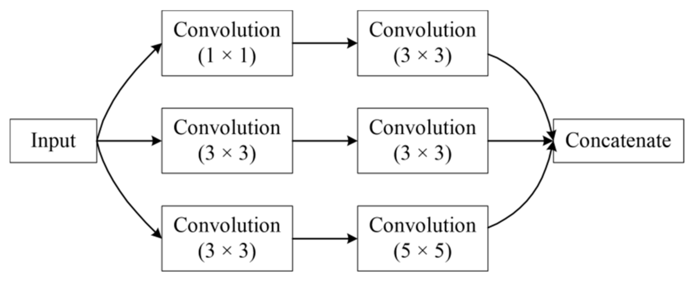
The convolution kernel size increases directly with input size. Figure 13 showed that different k-value-based multiscale convolutional modules yielded different results. Moreover, the 3M-CNN-Magnify model outperformed the others. They both demonstrated that the multiscale convolution kernel contributes to classification performance.
While the 3M-CNN model was slightly inferior to the single-scale CNN model, this was due to a small multiscale kernel k-value of 1, which was unsuitable for a large input size of 51.

5.4. Comparison with Different Methods

To assess the effectiveness of the 3M-CNN-Magnify model, a series of comparison experiments were conducted. Traditional MLAs-based models, such as RF, SVM, and FS-RF, etc., and DBN-based models, were selected. As shown in Table 4, the 3M-CNN-Magnify model achieved the highest average OA value, which was significantly higher than that of the MLAs-based OAs, and slightly higher than that of the DBN-based OAs.
The results showed that the strategy of multiscale kernels, coupled with various input sizes for different data, could contribute significantly to the extraction of the representative classification features.
Table 4 indicates that the training time of the 3M-CNN models was slightly longer than that of the MLAs- and DBN-based models. However, the time for parameter selection of some MLAs-based models was greater. For example, there were 80 groups of parameter combinations for SVM-based models. The time of parameter selection for DBN-SVM was also greater, which contained the selection of DBN’s and SVM’s parameters. Using less time, DBN-SVM yielded comparative OA with that of the 3M-CNN models. On the one hand, the coding layers based on feature vectors were much quicker than the convolution layers obtained by feature maps. On the other hand, the test accuracies were based on only a small set of samples, i.e., with 500 for each class. Therefore, the comparative test accuracies cannot reflect the true performances of the DBN-SVM and 3M-CNN models. The assessments of the predicted maps demonstrated that the 3M-CNN models were significantly better than the DBN-SVM model.
Three larger test sets were then used to further compare the model performances. Table 7 shows the accuracy values. From Figure 7, the following conclusions can be drawn: (1) With greater test sets, CNN-based models obtained greater accuracy values (about 3% improvement). This might be attributed to the overlap of 15 pixels × 15 pixels neighbors. However, the accuracies for those three test sets were stable, showing that the accuracy values for CNN-based models were reliable; (2) With greater test sets, DBN-based models’ accuracy values were slightly reduced; (3) With greater test sets, CNN-based models yielded about 4.7% improvement compared to DBN-based models. In the future, spatially independent test sets [9] will be constructed for model comparison.

5.5. Parameter Selection and Effects of the Dataset

The selection of input size of DEM data and corresponding kernel size was strictly conducted. However, the tuning of the baseline was very simple. For example, the input size of spectral images was determined based on subjective experience and the size of different land covers in the study area. In the single-scale CNN models, the numbers of convolution flows and fully connected layers were determined by a trial-and-error method.
The datasets in this study were not very large, containing only 2000, 500, and 500 samples for each class in the training, validation, and test sets, respectively. Therefore, the baseline of the single-scale CNN model was not complex, which helps avoid underfitting. The small performance gains among 3M-CNN-Magnify, single-scale CNN, and DBN-SVM models, might be partly caused by the small size of the datasets and their spatial auto-correlation [9] (see the subset area of 6 in Figure 6), which reached precision saturation. However, the map accuracies of the whole study area were far from optimal and showed obvious differences. As a result, larger spatial independent datasets should be investigated in the future.

5.6. Investigations on Different Datasets

A lot of time is needed to label the polygons for extracting training, validation, and test sets; consequently, our former studies [9,12,13,18] relied on only one dataset, i.e., the ZY-3 imagery on 20 June 2012.
The following features contributed to the reliability of the accuracy assessment results: (1) The training, validation, and test sets containing 2000, 500, and 500 samples for each class, respectively, were spatially independent (only 12.88% pixels in the data polygons were used on average (Table 2) [9]; (2) There were five groups of training, validation, and test sets, and each was run 5 times; (3) The study area was very large, i.e., 104.9 km2; (4) The classification maps were visually accurate.
However, it was considered of benefit to also investigate using other datasets (e.g., different imageries for different study areas), or ZY-3 datasets of this study at other times. As a result, the ZY-3 imagery on 11 November 2020 was further tested in this study. By directly using the model structures and hyper-parameters derived from the imagery on 20 June 2012, the imagery on 11 November 2020 yielded very high test accuracy values and accurate visual maps of LCC and FLCC. In future, imageries from different sources, geographical locations, and with varying spatial resolutions, should be further investigated to test the generalization capability of the proposed models.

6. Conclusions

A 3M-CNN model was proposed for FLCC of a CSMA in Wuhan City, China. ZY-3 imagery-derived true color, false color, and DEM data were fed into a multistream structure. The DEM data had different input neighbors with other data for better feature learning. A multiscale kernel was revised from the inception module. By testing two scenes of ZY-3 imageries, results indicated that: (1) a multistream CNN structure contributed significantly to the extraction of effective features from multimodal data; (2) with respect to CSMAs, optimal input neighbors and corresponding multiscale convolution kernels for the branch using DEM as input were crucial. In general, the proposed model achieved optimal performance and surpassed all other models. In the future, we will focus on the utilization of various imageries from different study areas, sources, spatial resolutions, and spatial independence, and with larger datasets. Furthermore, conduction of transfer learning from one dataset to another is worthy of further examination.

Author Contributions

All authors made significant contributions to the manuscript. Conceptualization, M.Q., S.S. and X.L.; formal analysis, M.Q., S.S. and X.L.; investigation, M.Q. and S.S.; methodology, M.Q., S.S. and X.L.; software, M.Q. and S.S.; supervision, X.L.; validation, M.Q. and S.S.; writing—original draft, M.Q. and S.S.; writing—review & editing, X.L. All authors have read and agreed to the published version of the manuscript.

Funding

This research received no external funding.

Data Availability Statement

Not applicable.

Conflicts of Interest

The authors declare no conflict of interest.

References

  1. DeFries, R.S.; Belward, A.S. Global and regional land cover characterization from satellite data: An introduction to the Special Issue. Int. J. Remote Sens. 2000, 21, 1083–1092. [Google Scholar] [CrossRef]
  2. Cihlar, J. Land cover mapping of large areas from satellites: Status and research priorities. Int. J. Remote Sens. 2000, 21, 1093–1114. [Google Scholar] [CrossRef]
  3. Maxwell, A.E.; Warner, T.A. Differentiating mine-reclaimed grasslands from spectrally similar land cover using terrain variables and object-based machine learning classification. Int. J. Remote Sens. 2015, 36, 4384–4410. [Google Scholar] [CrossRef] [Green Version]
  4. Myint, S.W.; Gober, P.; Brazel, A.; Grossman-Clarke, S.; Weng, Q. Per-pixel vs. object-based classification of urban land cover extraction using high spatial resolution imagery. Remote Sens. Environ. 2011, 115, 1145–1161. [Google Scholar] [CrossRef]
  5. Senf, C.; Leitão, P.J.; Pflugmacher, D.; van der Linden, S.; Hostert, P. Mapping land cover in complex Mediterranean landscapes using Landsat: Improved classification accuracies from integrating multi-seasonal and synthetic imagery. Remote Sens. Environ. 2015, 156, 527–536. [Google Scholar] [CrossRef]
  6. Silveyra Gonzalez, R.; Latifi, H.; Weinacker, H.; Dees, M.; Koch, B.; Heurich, M. Integrating LiDAR and high-resolution imagery for object-based mapping of forest habitats in a heterogeneous temperate forest landscape. Int. J. Remote Sens. 2018, 39, 8859–8884. [Google Scholar] [CrossRef]
  7. Yan, W.Y.; Shaker, A.; El-Ashmawy, N. Urban land cover classification using airborne LiDAR data: A review. Remote Sens. Environ. 2015, 158, 295–310. [Google Scholar] [CrossRef]
  8. Chen, W.; Li, X.; He, H.; Wang, L. A Review of Fine-Scale Land Use and Land Cover Classification in Open-Pit Mining Areas by Remote Sensing Techniques. Remote Sens. 2018, 10, 15. [Google Scholar] [CrossRef] [Green Version]
  9. Li, X.; Tang, Z.; Chen, W.; Wang, L. Multimodal and Multi-Model Deep Fusion for Fine Classification of Regional Complex Landscape Areas Using ZiYuan-3 Imagery. Remote Sens. 2019, 11, 22. [Google Scholar] [CrossRef] [Green Version]
  10. Pal, S.K.; Mitra, S. Multilayer perceptron, fuzzy sets, classification. IEEE Trans. Neural Netw. 1992, 3, 683–697. [Google Scholar] [CrossRef] [PubMed]
  11. Azeez, N.; Yahya, W.; Al-Taie, I.; Basbrain, A.; Clark, A. Regional Agricultural Land Classification Based on Random Forest (RF), Decision Tree, and SVMs Techniques; ICICT: London, UK, 2019; pp. 73–81. [Google Scholar]
  12. Li, X.; Chen, W.; Cheng, X.; Wang, L. A Comparison of Machine Learning Algorithms for Mapping of Complex Surface-Mined and Agricultural Landscapes Using ZiYuan-3 Stereo Satellite Imagery. Remote Sens. 2016, 8, 514. [Google Scholar] [CrossRef] [Green Version]
  13. Chen, W.; Li, X.; He, H.; Wang, L. Assessing Different Feature Sets’ Effects on Land Cover Classification in Complex Surface-Mined Landscapes by ZiYuan-3 Satellite Imagery. Remote Sens. 2018, 10, 23. [Google Scholar] [CrossRef] [Green Version]
  14. Chen, W.; Li, X.; Wang, L. Fine Land Cover Classification in an Open Pit Mining Area Using Optimized Support Vector Machine and WorldView-3 Imagery. Remote Sens. 2020, 12, 82. [Google Scholar] [CrossRef] [Green Version]
  15. Lv, Q.; Dou, Y.; Niu, X.; Xu, J.; Li, B. Classification of Land Cover Based on Deep Belief Networks Using Polarimetric RADARSAT-2 Data; IGARSS: Quebec, QC, Canada, 2014; pp. 4679–4682. [Google Scholar]
  16. Li, W.; Fu, H.; Yu, L.; Gong, P.; Feng, D.; Li, C.; Clinton, N. Stacked Autoencoder-based deep learning for remote-sensing image classification: A case study of African land-cover mapping. Int. J. Remote Sens. 2016, 37, 5632–5646. [Google Scholar] [CrossRef]
  17. Tong, X.; Xia, G.; Lu, Q.; Shen, H.; Li, S.; You, S.; Zhang, L. Land-cover classification with high-resolution remote sensing images using transferable deep models. Remote Sens. Environ. 2020, 237, 111322. [Google Scholar] [CrossRef] [Green Version]
  18. Li, M.; Tang, Z.; Tong, W.; Li, X.; Chen, W.; Wang, L. A Multi-Level Output-Based DBN Model for Fine Classification of Complex Geo-Environments Area Using Ziyuan-3 TMS Imagery. Sensors 2021, 21, 2089. [Google Scholar] [CrossRef] [PubMed]
  19. Liu, Y.; Huang, C. Scene Classification via Triplet Networks. IEEE J. Sel. Top. Appl. Earth Observ. Remote Sens. 2018, 11, 220–237. [Google Scholar] [CrossRef]
  20. Li, H.; Ghamisi, P.; Soergel, U.; Zhu, X. Hyperspectral and LiDAR Fusion Using Deep Three-Stream Convolutional Neural Networks. Remote Sens. 2018, 10, 1649. [Google Scholar] [CrossRef] [Green Version]
  21. Xu, X.; Li, W.; Ran, Q.; Du, Q.; Gao, L.; Zhang, B. Multisource Remote Sensing Data Classification Based on Convolutional Neural Network. IEEE Trans. Geosci. Remote Sens. 2018, 56, 937–949. [Google Scholar] [CrossRef]
  22. Chen, Y.; Li, C.; Ghamisi, P.; Shi, C.; Gu, Y. Deep Fusion of Hyperspectral and LiDAR Data for Thematic Classification; IGARSS: Beijing, China, 2016; pp. 3591–3594. [Google Scholar]
  23. Chen, Y.; Li, C.; Ghamisi, P.; Jia, X.; Gu, Y. Deep Fusion of Remote Sensing Data for Accurate Classification. IEEE Geosci. Remote Sens. Lett. 2017, 14, 1253–1257. [Google Scholar] [CrossRef]
  24. Jahan, F.; Zhou, J.; Awrangjeb, M.; Gao, Y. Fusion of Hyperspectral and LiDAR Data Using Discriminant Correlation Analysis for Land Cover Classification. IEEE J. Sel. Top. Appl. Earth Observ. Remote Sens. 2018, 11, 3905–3917. [Google Scholar] [CrossRef] [Green Version]
  25. Rasti, B.; Ghamisi, P.; Plaza, J.; Plaza, A. Fusion of Hyperspectral and LiDAR Data Using Sparse and Low-Rank Component Analysis. IEEE Trans. Geosci. Remote Sens. 2017, 55, 6354–6365. [Google Scholar] [CrossRef] [Green Version]
  26. Zhang, W.; Liljedahl, A.K.; Kanevskiy, M.; Epstein, H.E.; Jones, B.M.; Jorgenson, M.T.; Kent, K. Transferability of the deep learning mask R-CNN model for automated mapping of ice-wedge polygons in high-resolution satellite and UAV images. Remote Sens. 2020, 12, 1085. [Google Scholar] [CrossRef] [Green Version]
  27. Bhuiyan, M.A.E.; Witharana, C.; Liljedahl, A.K. Use of Very High Spatial Resolution Commercial Satellite Imagery and Deep Learning to Automatically Map Ice-Wedge Polygons across Tundra Vegetation Types. J. Imaging 2020, 6, 137. [Google Scholar] [CrossRef]
  28. Witharana, C.; Bhuiyan, M.A.E.; Liljedahl, A.K.; Kanevskiy, M.; Epstein, H.E.; Jones, B.M.; Daanen, R.; Griffin, C.G.; Kent, K.; Jones, M.K. Understanding the synergies of deep learning and data fusion of multispectral and panchromatic high resolution commercial satellite imagery for automated ice-wedge polygon detection. ISPRS-J. Photogramm. Remote Sens. 2020, 170, 174–191. [Google Scholar] [CrossRef]
  29. Yang, J.; Zhao, Y.Q.; Chan, J.C.W. Hyperspectral and Multispectral Image Fusion via Deep Two-Branches Convolutional Neural Network. Remote Sens. 2018, 10, 800. [Google Scholar] [CrossRef] [Green Version]
  30. Deur, M.; Gašparović, M.; Balenović, I. An Evaluation of Pixel- and Object-Based Tree Species Classification in Mixed Deciduous Forests Using Pansharpened Very High Spatial Resolution Satellite Imagery. Remote Sens. 2021, 13, 1868. [Google Scholar] [CrossRef]
  31. Zhang, S.; Li, C.; Qiu, S.; Gao, C.; Zhang, F.; Du, Z.; Liu, R. EMMCNN: An ETPS-Based Multi-Scale and Multi-Feature Method Using CNN for High Spatial Resolution Image Land-Cover Classification. Remote Sens. 2020, 12, 66. [Google Scholar] [CrossRef] [Green Version]
  32. Zhang, C.; Li, G.; Du, S. Multi-Scale Dense Networks for Hyperspectral Remote Sensing Image Classification. IEEE Trans. Geosci. Remote Sens. 2019, 57, 9201–9222. [Google Scholar] [CrossRef]
  33. Pontius, R.G.; Millones, M. Death to Kappa: Birth of quantity disagreement and allocation disagreement for accuracy assessment. Int. J. Remote Sens. 2011, 32, 4407–4429. [Google Scholar] [CrossRef]
Figure 1. ZiYuan-3 imagery on 20 June 2012 and field samples of the study area [12]. G107: national highway 107 of China.
Remotesensing 13 05052 g001
Figure 2. ZiYuan-3 imagery on 11 November 2020.
Remotesensing 13 05052 g002
Figure 3. Comparison of a sub-area from the two images. The red ellipses are the places with large changes.
Remotesensing 13 05052 g003
Figure 4. The overall framework of the multimodal data and multiscale kernel-based multistream convolutional neural network model. N1 × N1 and N2 × N2 represent the input neighbors. BN, batch normalization; ReLU, rectified linear unit.
Remotesensing 13 05052 g004
Figure 5. The demonstration area for explaining the utilization of 15 pixels × 15 pixels neighbor.
Remotesensing 13 05052 g005
Figure 6. The subset areas for explaining the utilization of 15 pixels × 15 pixels neighbor. 1: surface-mined land covers and mine pit pond; 2: road; 3: residential lands; 4: croplands; 5: paddy; 6: fallow land; 7: forest lands; 8: pond and stream. For data polygon and sample points, see Section 3.3.
Remotesensing 13 05052 g006
Figure 7. Details of the multiscale convolutional module 1.
Remotesensing 13 05052 g007
Figure 8. Details of the multiscale convolutional module 2.
Remotesensing 13 05052 g008
Figure 9. The diagram of extracting training, validation, and test samples.
Remotesensing 13 05052 g009
Figure 10. Overall framework of the single-scale convolutional neural network. The single-scale convolution flow is depicted in Figure 11. BN, batch normalization; ReLU, rectified linear unit; Dropout, a method to improve generalization performance.
Remotesensing 13 05052 g010
Figure 11. The details of the single-scale convolution flow. BN, batch normalization; ReLU, rectified linear unit.
Remotesensing 13 05052 g011
Figure 12. Training time and overall accuracy (OA) for the experiment of input size selection.
Remotesensing 13 05052 g012
Figure 13. Training time and overall accuracy (OA) for Experiment 2.
Remotesensing 13 05052 g013
Figure 14. The predicted maps of fine land cover classification with 20 classes based on the model of deep belief network and support vector machine in [9] and the multimodal data and multiscale kernel-based multistream convolutional neural network with selected value of parameter k and ZiYuan-3 imagery on 20 June 2012.
Remotesensing 13 05052 g014
Figure 15. The predicted maps of land cover classification with 7 classes based on the model of deep belief network and support vector machine in [9] and the multimodal data and multiscale kernel-based multistream convolutional neural network with selected value of parameter k and ZiYuan-3 imagery on 20 June 2012.
Remotesensing 13 05052 g015
Figure 16. The predicted maps of fine land cover classification and land cover classification based on the multimodal data and multiscale kernel-based multistream convolutional neural network with selected value of parameter k and ZY-3 imagery on 11 November 2020.
Remotesensing 13 05052 g016
Figure 17. The diagram of the proposed pipeline.
Remotesensing 13 05052 g017
Table 1. Characteristics of ZiYuan-3 satellite imagery [9,12]. PAN, panchromatic; GSD, ground spatial distance; MS, multispectral; NIR, near-infrared.
Sensor and Data FeaturesZiYuan-3 Satellite Imagery
Sensors and spatial resolutionnadir-looking PAN: 2.1 m GSD
front looking/backward looking PAN: 3.6 m GSD
nadir-looking MS: 5.8 m GSD
Spectral resolutionPAN (450–800 nm)
Blue (450–520 nm)
Green (520–590 nm)
Red (630–690 nm)
NIR (770–890 nm)
Radiometric resolution10-bit
Revisit cycle5 days
Table 2. Area (km2) of data polygons and fractions (%) of all training, validation, and test samples and data polygons, for details see reference [9].
ClassAreaFractionClassAreaFraction
Paddy0.149.61Dark road0.0623.66
Greenhouse0.0525.33Bright road0.0622.21
Green dry land0.158.87Light gray road0.139.96
Fallow land0.542.45Bright roof0.452.91
Woodland0.542.44Red roof0.0526.09
Shrubbery0.542.45Blue roof0.0528.61
Coerced forest0.139.96Bare surface0.187.55
Nursery0.197.11Open pit0.139.84
Pond and stream0.911.45Ore processing site0.139.95
Mine pit pond0.0527.60Dumping ground0.0719.57
Table 3. Models for comparison. CNN, convolutional neural network; 3M-CNN, multimodal data and multiscale kernel-based multistream CNN.
ModelDescription
Single-scale CNNWith just 3 × 3 convolutional kernels.
3M-CNNMultiscale kernels with k of 1.
3M-CNN-MagnifyMultiscale kernels with selected value of parameter k.
Table 4. Results of different models’ accuracy assessment. OA, overall accuracy; QD, quantity disagreement; AD, allocation disagreement; SVM, support vector machine; RF, random forest; DBN-S: deep belief network with softmax classifier; DBN-SVM, DBN with SVM as classifier; DBN-RF, DBN with RF as classifier; FS-SVM, combination of feature selection and SVM; CNN, convolutional neural network; 3M-CNN, multimodal data and multiscale kernel-based multistream CNN; 3M-CNN-Magnify, 3M-CNN with selected value of parameter k.
ModelOA (%)Time (h)QD (%)AD (%)
SVM [9]77.88% ± 0.53%0.59
RF [9]88.90% ± 0.20%0.22
DBN-S [9]94.23% ± 0.67%0.88
DBN-SVM [9]94.74% ± 0.35%1.01
DBN-RF [9]94.07% ± 0.34%1.06
FS-SVM [9]90.39% ± 0.42%2.11
Single-scale CNN94.79% ± 0.60%1.722.93% ± 0.31%2.35% ± 0.62%
3M-CNN94.40% ± 0.14%1.933.29% ± 0.28%2.40% ± 0.39%
3M-CNN-Magnify95.09% ± 0.29%1.793.16% ± 0.25%1.84% ± 0.22%
Table 5. Results of different models’ accuracy assessment for imagery on 11 November 2020. OA, overall accuracy; QD, quantity disagreement; AD, allocation disagreement; CN, convolutional neural network; 3M-CNN, multimodal data and multiscale kernel-based multistream CNN; 3M-CNN-Magnify, 3M-CNN with selected value of parameter k.
ModelOA (%)QD (%)AD (%)
Single-scale CNN93.76% ± 0.76%1.72% ± 0.49%4.48% ± 0.41%
3M-CNN95.11% ± 0.48%1.14% ± 0.14%3.73% ± 0.35%
3M-CNN-Magnify96.60% ± 0.22%0.91% ± 0.13%2.47% ± 0.15%
Table 6. Different models’ overall accuracy (OA) values for imagery on 20 June 2012. (1) CNN4321 DEM: a convolutional neural network (CNN) model with an input of both four spectral bands and digital elevation model (DEM) data; (2) CNN4321 + DEM: a CNN model with two inputs of four spectral bands and DEM data; (3) CNN321 + 432 + DEM: a CNN model with three inputs of true color image, false color image, and DEM data, respectively.
ModelOA (%)
CNN4321 DEM92.99% ± 0.39%
CNN4321 + DEM93.74% ± 0.48%
CNN321 + 432 + DEM94.32% ± 0.42%
Table 7. The accuracy values for three larger test sets. OA, overall accuracy; QD, quantity disagreement; AD, allocation disagreement; DBN-S, deep belief network with softmax classifier; DBN-SVM, DBN with support vector machine as classifier; CNN, convolutional neural network; 3M-CNN, multimodal data and multiscale kernel-based multistream CNN; 3M-CNN-Magnify, 3M-CNN with selected value of parameter k.
ModelOA (%)QD (%)AD (%)
The test set with 1000 samples for each class
DBN-S93.55% ± 0.02%1.01% ± 0.08%5.45% ± 0.08%
DBN-SVM93.73% ± 0.07%0.91% ± 0.05%5.38% ± 0.03%
Single-scale CNN97.11% ± 0.16%0.83% ± 0.14%2.06% ± 0.13%
3M-CNN97.41% ± 0.09%0.64% ± 0.14%1.95% ± 0.15%
3M-CNN-Magnify98.01% ± 0.18%0.52% ± 0.06%1.47% ± 0.15%
The test set with 1500 samples for each class
DBN-S93.72% ± 0.08%0.98% ± 0.06%5.30% ± 0.09%
DBN-SVM93.92% ± 0.05%0.89% ± 0.04%5.20% ± 0.02%
Single-scale CNN97.27% ± 0.13%0.73% ± 0.06%2.00% ± 0.13%
3M-CNN97.48% ± 0.12%0.64% ± 0.09%1.89% ± 0.15%
3M-CNN-Magnify98.05% ± 0.10%0.46% ± 0.03%1.48% ± 0.11%
The test set with 2000 samples for each class
DBN-S93.61% ± 0.10%0.95% ± 0.09%5.43% ± 0.14%
DBN-SVM93.80% ± 0.11%0.81% ± 0.10%5.40% ± 0.16%
Single-scale CNN97.18% ± 0.13%0.77% ± 0.10%2.05% ± 0.10%
3M-CNN97.40% ± 0.09%0.68% ± 0.08%1.92% ± 0.08%
3M-CNN-Magnify98.06% ± 0.15%0.45% ± 0.03%1.49% ± 0.12%
Publisher’s Note: MDPI stays neutral with regard to jurisdictional claims in published maps and institutional affiliations.

