
Single-Image Super-Resolution of Sentinel-2 Low Resolution Bands with Residual Dense Convolutional Neural Networks


Abstract
:
1. Introduction
2. Related Works
3. Materials and Methods
3.1. Dataset
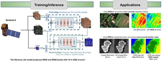
3.2. Proposed Model
3.2.1. Network Architecture
3.2.2. Training Details
3.3. Quantitative Metrics
- Root Mean Square Error (RMSE): measures the mean error in the pixel-value space.
- Signal to Reconstruction Ratio Error (SRE) [4]: measures the relative error in reference to the power of the signal, in dB, where the higher, the better (n is the number of pixels).
- Spectral Angle Mapper (SAM) [45]: measures the spectral fidelity between two images. It is expressed in radians, where smaller angles represent higher similarities.
- Peak Signal to Noise Ratio (PSNR): it is one of the standard metrics used to evaluate the quality of a reconstructed image. Here, MaxVal takes the maximum value of Y. Higher PSNR, generally, indicates higher quality.
- Structural Similarity (SSIM) [46]: measures the similarity of two images by considering three aspects: luminance, contrast, and structure. SSIM takes in consideration the mean () and variance () of the images, where a value of 1 corresponds to identical images. Constants and are values that depend on the dynamic range (L) of pixel values ( and are used by default).
- Erreur relative globale adimensionnelle de systhese (ERGAS) [47]: measures the quality of the reconstructed image considering the scaling factor (S) and the normalized error per each channel (B). Lower values imply higher quality.
4. Results
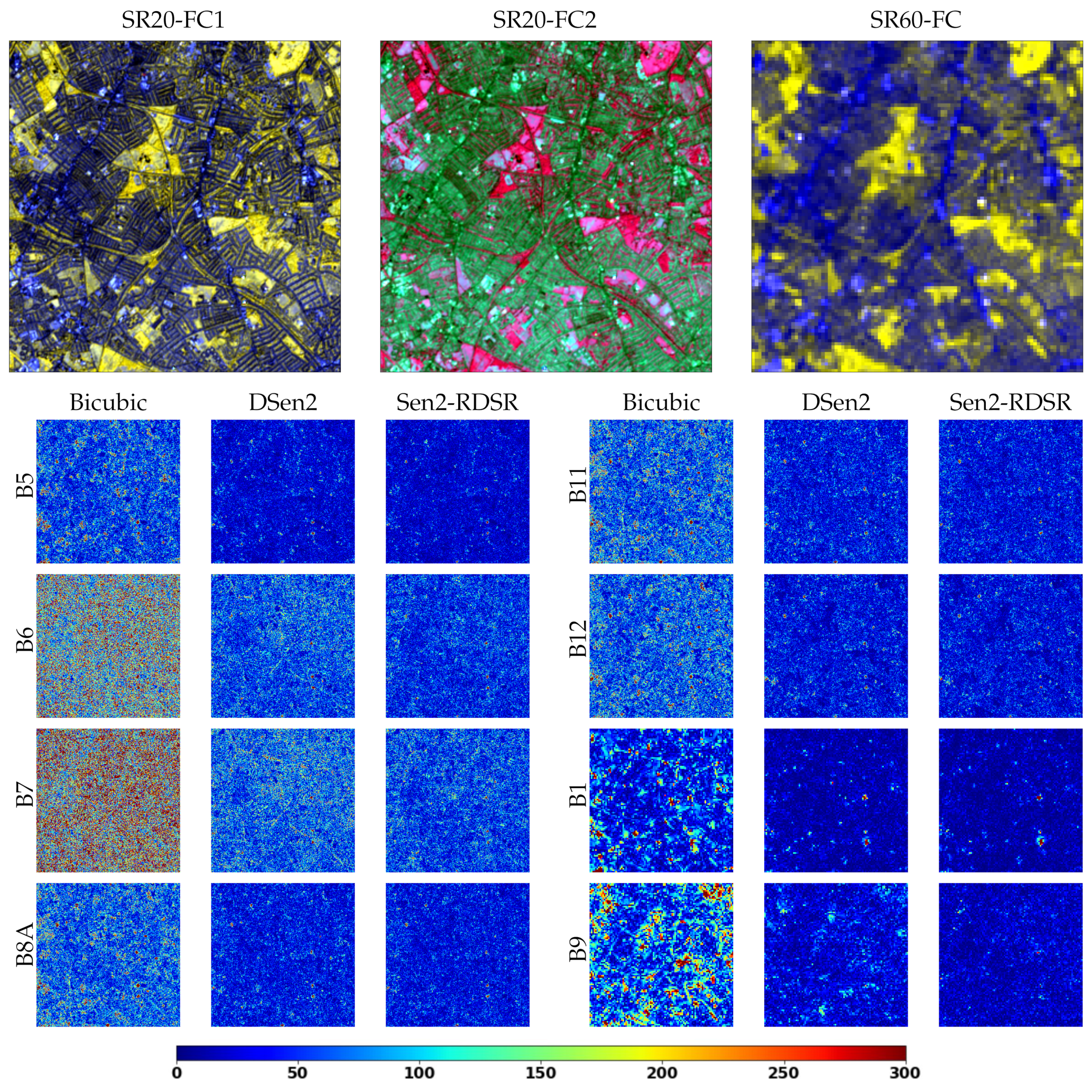
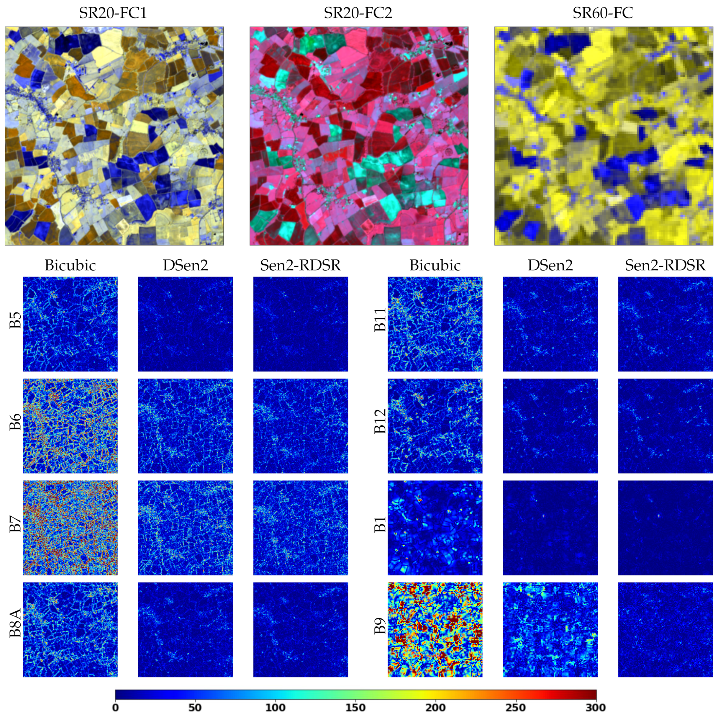
4.1. Super-Resolution Results
4.2. Applications
5. Discussion
6. Conclusions
Author Contributions
Funding
Institutional Review Board Statement
Informed Consent Statement
Data Availability Statement
Acknowledgments
Conflicts of Interest
Abbreviations
| ATPRK | Area to Point Regression Krigging |
| CNN | Convolutional Neural Network |
| DNN | Deep Neural Network |
| ESA | European Space Agency |
| GAN | Generative Adversarial Network |
| GSD | Ground Sampling Distance |
| HR | High-Resolution |
| IR | Infrared |
| LULC | Land Use Land Cover |
| LR | Low-Resolution |
| MS | Multi-Spectral |
| NDVI | Normalized Difference Vegetation Index |
| NDVI-RE | Normalized Difference Vegetation Index Red-edge |
| NMDI | Normalized Multi-band Drought Index |
| PAN | Panchromatic band |
| PSNR | Peak Signal to Noise Ratio |
| RMSE | Root Mean Square Error |
| RRDB | Residual in Residual Dense Block |
| SAM | Spectral Angle Mapper |
| Sen2-RDSR | Sentinel-2 Residual Dense Super-Resolution |
| SISR | Single-Image Super-Resolution |
| SR | Super-Resolution |
| SRCNN | Super-Resolution Convolutional Neural Network |
| SRE | Signal to Reconstruction Ratio Error |
| SSIM | Structural Similarity |
| SVM | Support Vector Machine |
| SWIR | Short-Wave Infrared |
| SR20 | Super-Resolution of 20 m bands |
| SR60 | Super-Resolution of 60 m bands |
| TB | TeraByte |
| VDSR | Very Deep Super-Resolution |
| VIS-NIR | Visible and Near Infrared |
| VLR | Very-Low Resolution |
References
- Drusch, M.; Del Bello, U.; Carlier, S.; Colin, O.; Fernandez, V.; Gascon, F.; Hoersch, B.; Isola, C.; Laberinti, P.; Martimort, P.; et al. Sentinel-2: ESA’s optical high-resolution mission for GMES operational services. Remote Sens. Environ. 2012, 120, 25–36. [Google Scholar] [CrossRef]
- Copernicus Open Access Hub. European Space Agency. Available online: https://scihub.copernicus.eu/dhus/#/home (accessed on 21 March 2021).
- Zhang, R.; Cavallaro, G.; Jitsev, J. Super-Resolution of Large Volumes of Sentinel-2 Images with High Performance Distributed Deep Learning. In Proceedings of the IGARSS 2020—2020 IEEE International Geoscience and Remote Sensing Symposium, Waikoloa, HI, USA, 26 September–2 October 2020; pp. 617–620. [Google Scholar] [CrossRef]
- Lanaras, C.; Bioucas-Dias, J.; Galliani, S.; Baltsavias, E.; Schindler, K. Super-resolution of Sentinel-2 images: Learning a globally applicable deep neural network. ISPRS J. Photogramm. Remote Sens. 2018, 146, 305–319. [Google Scholar] [CrossRef] [Green Version]
- Alparone, L.; Aiazzi, B.; Baronti, S.; Garzelli, A. Remote Sensing Image Fusion; CRC Press: Boca Raton, FL, USA, 2015. [Google Scholar]
- Lillesand, T.; Kiefer, R.W.; Chipman, J. Remote Sensing and Image Interpretation; John Wiley & Sons: Hoboken, NJ, USA, 2015. [Google Scholar]
- Liebel, L.; Körner, M. Single-image super resolution for multispectral remote sensing data using convolutional neural networks. ISPRS-Int. Arch. Photogramm. Remote Sens. Spat. Inf. Sci. 2016, 41, 883–890. [Google Scholar] [CrossRef] [Green Version]
- Wagner, L.; Liebel, L.; Körner, M. Deep residual learning for single-image super-resolution of multi-spectral satellite imagery. ISPRS Ann. Photogramm. Remote Sens. Spat. Inf. Sci. 2019, 4. [Google Scholar] [CrossRef] [Green Version]
- Toming, K.; Kutser, T.; Laas, A.; Sepp, M.; Paavel, B.; Nõges, T. First experiences in mapping lake water quality parameters with Sentinel-2 MSI imagery. Remote Sens. 2016, 8, 640. [Google Scholar] [CrossRef] [Green Version]
- Kolokoussis, P.; Karathanassi, V. Oil spill detection and mapping using sentinel 2 imagery. J. Mar. Sci. Eng. 2018, 6, 4. [Google Scholar] [CrossRef] [Green Version]
- Phiri, D.; Simwanda, M.; Salekin, S.; Nyirenda, V.R.; Murayama, Y.; Ranagalage, M. Sentinel-2 data for land cover/use mapping: A review. Remote Sens. 2020, 12, 2291. [Google Scholar] [CrossRef]
- Pedrayes, O.D.; Lema, D.G.; García, D.F.; Usamentiaga, R.; Alonso, Á. Evaluation of Semantic Segmentation Methods for Land Use with Spectral Imaging Using Sentinel-2 and PNOA Imagery. Remote Sens. 2021, 13, 2292. [Google Scholar] [CrossRef]
- Anwar, S.; Khan, S.; Barnes, N. A deep journey into super-resolution: A survey. ACM Comput. Surv. (CSUR) 2020, 53, 1–34. [Google Scholar] [CrossRef]
- Arefin, M.R.; Michalski, V.; St-Charles, P.L.; Kalaitzis, A.; Kim, S.; Kahou, S.E.; Bengio, Y. Multi-image super-resolution for remote sensing using deep recurrent networks. In Proceedings of the IEEE/CVF Conference on Computer Vision and Pattern Recognition Workshops, Seattle, WA, USA, 14–19 June 2020; pp. 206–207. [Google Scholar]
- Tsagkatakis, G.; Aidini, A.; Fotiadou, K.; Giannopoulos, M.; Pentari, A.; Tsakalides, P. Survey of deep-learning approaches for remote sensing observation enhancement. Sensors 2019, 19, 3929. [Google Scholar] [CrossRef] [Green Version]
- Zhu, X.; Xu, Y.; Wei, Z. Super-Resolution of Sentinel-2 Images Based on Deep Channel-Attention Residual Network. In Proceedings of the IGARSS 2019-2019 IEEE International Geoscience and Remote Sensing Symposium, Yokohama, Japan, 28 July–2 August 2019; pp. 628–631. [Google Scholar]
- Salgueiro Romero, L.; Marcello, J.; Vilaplana, V. Super-Resolution of Sentinel-2 Imagery Using Generative Adversarial Networks. Remote Sens. 2020, 12, 2424. [Google Scholar] [CrossRef]
- Zhou, C.; Zhang, J.; Liu, J.; Zhang, C.; Fei, R.; Xu, S. PercepPan: Towards unsupervised pan-sharpening based on perceptual loss. Remote Sens. 2020, 12, 2318. [Google Scholar] [CrossRef]
- Kaplan, G. Sentinel-2 Pan Sharpening—Comparative Analysis. Proceedings 2018, 2, 345. [Google Scholar] [CrossRef] [Green Version]
- Vaiopoulos, A.; Karantzalos, K. Pansharpening on the narrow VNIR and SWIR spectral bands of Sentinel-2. Int. Arch. Photogramm. Remote Sens. Spat. Inf. Sci. 2016, 41, 723. [Google Scholar] [CrossRef] [Green Version]
- Du, Y.; Zhang, Y.; Ling, F.; Wang, Q.; Li, W.; Li, X. Water bodies’ mapping from Sentinel-2 imagery with modified normalized difference water index at 10-m spatial resolution produced by sharpening the SWIR band. Remote Sens. 2016, 8, 354. [Google Scholar] [CrossRef] [Green Version]
- Gašparović, M.; Jogun, T. The effect of fusing Sentinel-2 bands on land-cover classification. Int. J. Remote Sens. 2018, 39, 822–841. [Google Scholar] [CrossRef]
- Armannsson, S.E.; Ulfarsson, M.O.; Sigurdsson, J.; Nguyen, H.V.; Sveinsson, J.R. A Comparison of Optimized Sentinel-2 Super-Resolution Methods Using Wald’s Protocol and Bayesian Optimization. Remote Sens. 2021, 13, 2192. [Google Scholar] [CrossRef]
- Brook, A.; De Micco, V.; Battipaglia, G.; Erbaggio, A.; Ludeno, G.; Catapano, I.; Bonfante, A. A smart multiple spatial and temporal resolution system to support precision agriculture from satellite images: Proof of concept on Aglianico vineyard. Remote Sens. Environ. 2020, 240, 111679. [Google Scholar] [CrossRef]
- Wang, Q.; Shi, W.; Li, Z.; Atkinson, P.M. Fusion of Sentinel-2 images. Remote Sens. Environ. 2016, 187, 241–252. [Google Scholar] [CrossRef] [Green Version]
- Brodu, N. Super-resolving multiresolution images with band-independent geometry of multispectral pixels. IEEE Trans. Geosci. Remote Sens. 2017, 55, 4610–4617. [Google Scholar] [CrossRef] [Green Version]
- Zhang, K.; Sumbul, G.; Demir, B. An Approach To Super-Resolution Of Sentinel-2 Images Based On Generative Adversarial Networks. In Proceedings of the 2020 Mediterranean and Middle-East Geoscience and Remote Sensing Symposium (M2GARSS), Tunis, Tunisia, 9–11 March 2020; pp. 69–72. [Google Scholar]
- Goodfellow, I.J.; Pouget-Abadie, J.; Mirza, M.; Xu, B.; Warde-Farley, D.; Ozair, S.; Courville, A.; Bengio, Y. Generative adversarial networks. arXiv 2014, arXiv:1406.2661. [Google Scholar] [CrossRef]
- Zhang, Y.; Li, K.; Li, K.; Wang, L.; Zhong, B.; Fu, Y. Image super-resolution using very deep residual channel attention networks. In Proceedings of the European Conference on Computer Vision (ECCV), Munich, Germany, 8–14 September 2018; pp. 286–301. [Google Scholar]
- Dong, C.; Loy, C.C.; He, K.; Tang, X. Image super-resolution using deep convolutional networks. IEEE Trans. Pattern Anal. Mach. Intell. 2015, 38, 295–307. [Google Scholar] [CrossRef] [Green Version]
- Kim, J.; Lee, J.K.; Lee, K.M. Accurate image super-resolution using very deep convolutional networks. In Proceedings of the IEEE Conference on Computer Vision and Pattern Recognition, Las Vegas, NV, USA, 27–30 June 2016; pp. 1646–1654. [Google Scholar]
- Palsson, F.; Sveinsson, J.R.; Ulfarsson, M.O. Sentinel-2 image fusion using a deep residual network. Remote Sens. 2018, 10, 1290. [Google Scholar] [CrossRef] [Green Version]
- Ledig, C.; Theis, L.; Huszar, F.; Caballero, J.; Cunningham, A.; Acosta, A.; Aitken, A.; Tejani, A.; Totz, J.; Wang, Z.; et al. Photo-Realistic Single Image Super-Resolution Using a Generative Adversarial Network. In Proceedings of the IEEE Conference on Computer Vision and Pattern Recognition (CVPR), Honolulu, HI, USA, 22–25 July 2017. [Google Scholar]
- Gargiulo, M.; Mazza, A.; Gaetano, R.; Ruello, G.; Scarpa, G. Fast super-resolution of 20 m Sentinel-2 bands using convolutional neural networks. Remote Sens. 2019, 11, 2635. [Google Scholar] [CrossRef] [Green Version]
- Wu, J.; He, Z.; Hu, J. Sentinel-2 Sharpening via parallel residual network. Remote Sens. 2020, 12, 279. [Google Scholar] [CrossRef] [Green Version]
- Wang, X.; Yu, K.; Wu, S.; Gu, J.; Liu, Y.; Dong, C.; Qiao, Y.; Change Loy, C. Esrgan: Enhanced super-resolution generative adversarial networks. In Proceedings of the European Conference on Computer Vision (ECCV) Workshops, Munich, Germany, 8–14 September 2018. [Google Scholar]
- MultiSpectral Instrument (MSI) Overview. Available online: https://sentinels.copernicus.eu/web/sentinel/technical-guides/sentinel-2-msi/msi-instrument (accessed on 26 November 2021).
- Sentinel-2 User Handbook. Available online: https://sentinel.esa.int/documents/247904/685211/Sentinel-2_User_Handbook (accessed on 21 March 2021).
- Wald, L.; Ranchin, T.; Mangolini, M. Fusion of satellite images of different spatial resolutions: Assessing the quality of resulting images. Photogramm. Eng. Remote Sens. 1997, 63, 691–699. [Google Scholar]
- Szegedy, C.; Ioffe, S.; Vanhoucke, V.; Alemi, A. Inception-v4, inception-resnet and the impact of residual connections on learning. In Proceedings of the AAAI Conference on Artificial Intelligence, San Francisco, CA, USA., 4’9 February 2017; Volume 31. [Google Scholar]
- Chen, H.; Zhang, X.; Liu, Y.; Zeng, Q. Generative adversarial networks capabilities for super-resolution reconstruction of weather radar echo images. Atmosphere 2019, 10, 555. [Google Scholar] [CrossRef] [Green Version]
- Romero, L.S.; Marcello, J.; Vilaplana, V. Comparative study of upsampling methods for super-resolution in remote sensing. In Proceedings of the Twelfth International Conference on Machine Vision (ICMV 2019), Amsterdam, The Netherlands, 16–18 November 2019; Volume 11433, p. 114331. [Google Scholar]
- Huang, G.; Liu, Z.; Van Der Maaten, L.; Weinberger, K.Q. Densely connected convolutional networks. In Proceedings of the IEEE Conference on Computer Vision and Pattern Recognition, Honolulu, HI, USA, 22–25 July 2017; pp. 4700–4708. [Google Scholar]
- Pascanu, R.; Mikolov, T.; Bengio, Y. On the difficulty of training recurrent neural networks. In Proceedings of the 30th International Conference on Machine Learning, Atlanta, GA, USA, 16–21 June 2013; pp. 1310–1318. [Google Scholar]
- Yuhas, R.H.; Goetz, A.F.; Boardman, J.W. Discrimination among semi-arid landscape endmembers using the spectral angle mapper (SAM) algorithm. In Proceedings of the Summaries 3rd Annu. JPL Airborne Geosci Workshop, Pasadena, CA, USA, 1–5 June 1992; Volume 1, pp. 147–149. [Google Scholar]
- Wang, Z.; Bovik, A.C.; Sheikh, H.R.; Simoncelli, E.P. Image quality assessment: From error visibility to structural similarity. IEEE Trans. Image Process. 2004, 13, 600–612. [Google Scholar] [CrossRef] [Green Version]
- Wald, L. Data Fusion: Definitions and Architectures: Fusion of Images of Different Spatial Resolutions; Presses des MINES: Paris, France, 2002. [Google Scholar]
- Camps-Valls, G.; Tuia, D.; Gómez-Chova, L.; Jiménez, S.; Malo, J. Remote sensing image processing. Synth. Lect. Image Video Multimed. Process. 2011, 5, 1–192. [Google Scholar] [CrossRef]
- Tarabalka, Y.; Chanussot, J.; Benediktsson, J.A. Segmentation and classification of hyperspectral images using watershed transformation. Pattern Recognit. 2010, 43, 2367–2379. [Google Scholar] [CrossRef] [Green Version]
- Signoroni, A.; Savardi, M.; Baronio, A.; Benini, S. Deep learning meets hyperspectral image analysis: A multidisciplinary review. J. Imaging 2019, 5, 52. [Google Scholar] [CrossRef] [PubMed] [Green Version]
- Li, S.; Song, W.; Fang, L.; Chen, Y.; Ghamisi, P.; Benediktsson, J.A. Deep learning for hyperspectral image classification: An overview. IEEE Trans. Geosci. Remote Sens. 2019, 57, 6690–6709. [Google Scholar] [CrossRef] [Green Version]
- Moliner, E.; Romero, L.S.; Vilaplana, V. Weakly Supervised Semantic Segmentation For Remote Sensing Hyperspectral Imaging. In Proceedings of the ICASSP 2020—2020 IEEE International Geoscience and Remote Sensing Symposium, Barcelona, Spain, 4–8 May 2020; pp. 2273–2277. [Google Scholar]
- Medina Machín, A.; Marcello, J.; Hernández-Cordero, A.I.; Martín Abasolo, J.; Eugenio, F. Vegetation species mapping in a coastal-dune ecosystem using high resolution satellite imagery. GIScience Remote Sens. 2019, 56, 210–232. [Google Scholar] [CrossRef]
- Maulik, U.; Chakraborty, D. Remote Sensing Image Classification: A survey of support-vector-machine-based advanced techniques. IEEE Geosci. Remote Sens. Mag. 2017, 5, 33–52. [Google Scholar] [CrossRef]
- Sheykhmousa, M.; Mahdianpari, M.; Ghanbari, H.; Mohammadimanesh, F.; Ghamisi, P.; Homayouni, S. Support Vector Machine vs. Random Forest for Remote Sensing Image Classification: A Meta-analysis and systematic review. IEEE J. Sel. Top. Appl. Earth Obs. Remote Sens. 2020, 13, 6308–6325. [Google Scholar] [CrossRef]
- Wang, L.; Qu, J.J. NMDI: A normalized multi-band drought index for monitoring soil and vegetation moisture with satellite remote sensing. Geophys. Res. Lett. 2007, 34, L20405. [Google Scholar] [CrossRef]
- Pan, H.; Chen, Z.; Ren, J.; Li, H.; Wu, S. Modeling winter wheat leaf area index and canopy water content with three different approaches using Sentinel-2 multispectral instrument data. IEEE J. Sel. Top. Appl. Earth Obs. Remote Sens. 2018, 12, 482–492. [Google Scholar] [CrossRef]
- Pereira-Pires, J.E.; Aubard, V.; Ribeiro, R.A.; Fonseca, J.M.; Silva, J.; Mora, A. Semi-automatic methodology for fire break maintenance operations detection with Sentinel-2 imagery and artificial neural network. Remote Sens. 2020, 12, 909. [Google Scholar] [CrossRef] [Green Version]
- Cucca, B.; Recanatesi, F.; Ripa, M.N. Evaluating the Potential of Vegetation Indices in Detecting Drought Impact Using Remote Sensing Data in a Mediterranean Pinewood. In International Conference on Computational Science and Its Applications; Springer: Berlin/Heidelberg, Germany, 2020; pp. 50–62. [Google Scholar]
- Sun, Y.; Qin, Q.; Ren, H.; Zhang, T.; Chen, S. Red-edge band vegetation indices for leaf area index estimation from Sentinel-2/msi imagery. IEEE Trans. Geosci. Remote Sens. 2019, 58, 826–840. [Google Scholar] [CrossRef]
- Lin, S.; Li, J.; Liu, Q.; Li, L.; Zhao, J.; Yu, W. Evaluating the effectiveness of using vegetation indices based on red-edge reflectance from Sentinel-2 to estimate gross primary productivity. Remote Sens. 2019, 11, 1303. [Google Scholar] [CrossRef] [Green Version]
- Evangelides, C.; Nobajas, A. Red-Edge Normalised Difference Vegetation Index NDVI705 from Sentinel-2 imagery to assess post-fire regeneration. Remote Sens. Appl. Soc. Environ. 2020, 17, 100283. [Google Scholar] [CrossRef]
- Marcello, J.; Eugenio, F.; Gonzalo-Martín, C.; Rodriguez-Esparragon, D.; Marqués, F. Advanced Processing of Multiplatform Remote Sensing Imagery for the Monitoring of Coastal and Mountain Ecosystems. IEEE Access 2020, 9, 6536–6549. [Google Scholar] [CrossRef]
- IEO (Instituto Español de Oceanografía). Parque Nacional Marítimo-Terrestre del Archipiélago de Cabrera (Data Source). Available online: http://www.ideo-cabrera.ieo.es/ (accessed on 13 April 2021).
- Ma, L.; Liu, Y.; Zhang, X.; Ye, Y.; Yin, G.; Johnson, B.A. Deep learning in remote sensing applications: A meta-analysis and review. ISPRS J. Photogramm. Remote Sens. 2019, 152, 166–177. [Google Scholar] [CrossRef]


| Spectral Band | S2A Central Wavelength (nm) | S2A Bandwidth * (nm) | S2B Central Wavelength (nm) | S2B Bandwidth * (nm) | Spatial Resolution GSD (m) |
|---|---|---|---|---|---|
| B1: Coastal Aerosol | 442.7 | 21 | 442.3 | 21 | 60 |
| B2: Blue | 492.4 | 66 | 492.1 | 66 | 10 |
| B3: Green | 559.8 | 36 | 559.0 | 36 | 10 |
| B4: Red | 664.6 | 31 | 665.0 | 31 | 10 |
| B5: Red-edge 1 | 704.1 | 15 | 703.8 | 16 | 20 |
| B6: Red-edge 2 | 740.5 | 15 | 703.8 | 15 | 20 |
| B7: Red-edge 3 | 782.8 | 20 | 779.7 | 20 | 20 |
| B8: Near-IR | 832.8 | 106 | 833.0 | 106 | 10 |
| B8A: Near-IR narrow | 864.7 | 21 | 864.0 | 22 | 20 |
| B9: Water Vapor | 945.1 | 20 | 943.2 | 21 | 60 |
| B10: SWIR-Cirrus | 1373.5 | 31 | 1376.9 | 30 | 60 |
| B11: SWIR-1 | 1613.7 | 91 | 1610.4 | 94 | 20 |
| B12: SWIR-2 | 2202.4 | 175 | 2185.7 | 185 | 20 |
| RMSE | SRE | SAM | PSNR | SSIM | ERGAS | |
|---|---|---|---|---|---|---|
| Bicubic | 125.68 | 26.44 | 1.21 | 45.82 | 0.82 | 3.33 |
| DSen2 [4] | 35.85 | 35.94 | 0.78 | 55.54 | 0.93 | 1.07 |
| Zhang et al. [3] | 34.99 | 36.19 | 0.75 | 55.77 | 0.93 | 1.03 |
| Sen2-RDSR | 34.38 | 36.38 | 0.75 | 55.94 | 0.93 | 1.02 |
| RMSE | SRE | SAM | PSNR | SSIM | ERGAS | |
|---|---|---|---|---|---|---|
| Bicubic | 162.16 | 19.77 | 1.78 | 37.66 | 0.35 | 2.43 |
| DSen2 [4] | 28.11 | 34.47 | 0.36 | 52.49 | 0.89 | 1.38 |
| Zhang et al. [3] | 26.80 | 34.98 | 0.34 | 52.94 | 0.90 | 1.29 |
| Sen2-RDSR | 25.69 | 35.14 | 0.34 | 52.10 | 0.90 | 0.41 |
| B5 | B6 | B7 | B8A | B11 | B12 | |
|---|---|---|---|---|---|---|
| RMSE | ||||||
| Bicubic | 101.23 | 133.35 | 153.96 | 87.37 | 74.14 | 162.34 |
| DSen2 [4] | 27.74 | 32.68 | 36.07 | 38.02 | 36.22 | 34.55 |
| Zhang et al. [3] | 27.48 | 32.27 | 35.58 | 37.46 | 35.56 | 33.68 |
| Sen2-RDSR | 26.98 | 35.95 | 41.28 | 27.62 | 24.78 | 42.01 |
| SRE | ||||||
| Bicubic | 25.42 | 25.89 | 25.66 | 26.80 | 24.44 | 25.81 |
| DSen2 [4] | 36.15 | 36.33 | 36.37 | 36.49 | 36.45 | 35.97 |
| Zhang et al. [3] | 36.26 | 36.44 | 36.49 | 36.62 | 36.66 | 36.22 |
| Sen2-RDSR | 36.46 | 36.96 | 36.87 | 36.76 | 37.26 | 36.76 |
Publisher’s Note: MDPI stays neutral with regard to jurisdictional claims in published maps and institutional affiliations. |
© 2021 by the authors. Licensee MDPI, Basel, Switzerland. This article is an open access article distributed under the terms and conditions of the Creative Commons Attribution (CC BY) license (https://creativecommons.org/licenses/by/4.0/).
Share and Cite
Salgueiro, L.; Marcello, J.; Vilaplana, V. Single-Image Super-Resolution of Sentinel-2 Low Resolution Bands with Residual Dense Convolutional Neural Networks. Remote Sens. 2021, 13, 5007. https://doi.org/10.3390/rs13245007
Salgueiro L, Marcello J, Vilaplana V. Single-Image Super-Resolution of Sentinel-2 Low Resolution Bands with Residual Dense Convolutional Neural Networks. Remote Sensing. 2021; 13(24):5007. https://doi.org/10.3390/rs13245007
Chicago/Turabian StyleSalgueiro, Luis, Javier Marcello, and Verónica Vilaplana. 2021. "Single-Image Super-Resolution of Sentinel-2 Low Resolution Bands with Residual Dense Convolutional Neural Networks" Remote Sensing 13, no. 24: 5007. https://doi.org/10.3390/rs13245007