Detecting Rock Glacier Displacement in the Central Himalayas Using Multi-Temporal InSAR

Abstract

Rock glaciers represent typical periglacial landscapes and are distributed widely in alpine mountain environments. Rock glacier activity represents a critical indicator of water reserves state, permafrost distribution, and landslide disaster susceptibility. The dynamics of rock glacier activity in alpine periglacial environments are poorly quantified, especially in the central Himalayas. Multi-temporal Interferometric Synthetic Aperture Radar (MT-InSAR) has been shown to be a useful technique for rock glacier deformation detection. In this study, we developed a multi-baseline persistent scatterer (PS) and distributed scatterer (DS) combined MT-InSAR method to monitor the activity of rock glaciers in the central Himalayas. In periglacial landforms, the application of the PS interferometry (PSI) method is restricted by insufficient PS due to large temporal baseline intervals and temporal decorrelation, which hinder comprehensive measurements of rock glaciers. Thus, we first evaluated the rock glacier interferometric coherence of all possible interferometric combinations and determined a multi-baseline network based on rock glacier coherence; then, we constructed a Delaunay triangulation network (DTN) by exploiting both PS and DS points. To improve the robustness of deformation parameters estimation in the DTN, we combined the Nelder–Mead algorithm with the M-estimator method to estimate the deformation rate variation at the arcs of the DTN and introduced a ridge-estimator-based weighted least square (WLR) method for the inversion of the deformation rate from the deformation rate variation. We applied our method to Sentinel-1A ascending and descending geometry data (May 2018 to January 2019) and obtained measurements of rock glacier deformation for 4327 rock glaciers over the central Himalayas, at least more than 15% detecting with single geometry data. The line-of-sight (LOS) deformation of rock glaciers in the central Himalayas ranged from −150 mm to 150 mm. We classified the active deformation area (ADA) of all individual rock glaciers with the threshold determined by the standard deviation of the deformation map. The results show that 49% of the detected rock glaciers (monitoring rate greater than 30%) are highly active, with an ADA ratio greater than 10%. After projecting the LOS deformation to the steep slope direction and classifying the rock glacier activity following the IPA Action Group guideline, 12% of the identified rock glaciers were classified as active and 86% were classified as transitional. This research is the first multi-baseline, PS, and DS network-based MT-InSAR method applied to detecting large-scale rock glaciers activity.

1. Introduction

Rock glacier is a tongue or lobate-shaped landform consisting of a seasonally frozen active rock debris layer, unconsolidated rock debris, and ice supersaturated debris or pure ice [1,2]. It is a typical gravity and seasonally freeze-thaw driven feature of creeping permafrost found in periglacial environments [3,4]. Due to the thermal insulating effect of unconsolidated rock debris, the melting of pure inner ice is retarded; thus, a rock glacier landform is more climatically resilient than a glacier and may prolong water storage in high mountain systems [5,6]. A rock glacier is of great hydrological importance in periglacial environments; the abundance of rock glaciers greatly influences the amount and properties of runoff from high mountain watersheds [3,7]. The water storage of rock glaciers provides a buffering capacity for surrounding lowlands [5]. Periglacial hydrological resources are susceptible to environmental change; the active layer thickness of rock glaciers and periglacial permafrost thickens as temperature increases [8,9,10]; the displacement variations of rock glaciers are effective indicators of periglacial environmental change [7,8]. Abnormally increasing rock glacier displacements can pose landslide hazards [8], and thus rock glacier surface creeping should be monitored for landslide hazard prevention [4]. In addition, the existence of active rock glaciers is an indicator of permafrost distribution. Detecting rock glacier activity is also crucial for mapping the permafrost zonation index [11,12].

In recent years, the surface displacements of rock glaciers have been monitored with field measurements [13], including by repeated geodetic tachymetric surveys (e.g., triangulation), in situ GNSS (global navigation satellite system) systems, and terrestrial laser scanning (or LiDAR) measurements [7,14,15]. These conventional methods are limited to sparse point densities and are extremely labor-intensive because of the remoteness of the locations and the complex climate and terrain environments [16], and generally they do not meet application requirements at the regional or continental scale [4,16]. Optical remote sensing techniques have been commonly used to generate regional inventories of rock glaciers [17]. Repeated stereo-imagery photogrammetry is an optional method for surface displacement monitoring of rock glaciers, allowing retrospective reconstruction of surface velocities over long periods [18]. Space-borne high-resolution optical images are normally used to identify the distribution of rock glaciers based on their distinct surface characteristics [19,20,21]. The activity of rock glaciers can only be classified qualitatively based on surface characteristics related to downslope deformations [19].

Compared with field-based or optical sensors methods, the use of synthetic aperture radar (SAR) and SAR interferometry (InSAR) is a more efficient alternative for investigating active landslides deformation, glacier movement [22,23], and the displacements of rock glaciers [24,25,26,27,28] due to the large coverage, high resolution, and frequent acquisitions. Differential InSAR (DInSAR) has been successfully applied to retrieve the surface motions of rock glaciers with a short temporal baseline [29,30,31,32,33,34]. However, the use of DInSAR for rock glacier deformation detection is limited by spatio-temporal decorrelation, geometric decorrelation, and atmospheric delay due to the complexity of periglacial environments [27]. To mitigate the limitations of DInSAR, multi-temporal InSAR (MT-InSAR), such as persistent scatter interferometry (PSI) [35], and the small baselines subset (SBAS) method [36] have been developed to monitor deformation rates and reconstruct the long-term cumulative ground movements of rock glaciers with millimeter-level accuracy [32,37,38,39,40,41,42]. Barboux et al. compared the applicability of PSI and SBAS for monitoring the deformation of high elevation periglacial environments [32]. Results showed that the PSI method had a higher deformation rate estimation accuracy in small areas but that the monitoring points were insufficient due to temporal decorrelation. Previous studies of rock glacier displacements measurements focused on relatively small spatial scales [43]. Systematic studies of the characteristics of regional rock glacier activity are still rare [44].

In the Himalayas, some studies monitored the deformation of rock glaciers using the SBAS method [43,45]. The deformation destabilization in some typical rock glacier regions was successfully detected; however, a quantitative deformation inventory of rock glaciers is still limited to few areas [43,44,45]. Reinosch et al. carried out a rock glacier activity inventory over the western Nyainqêntanglha range via InSAR time-series analysis with Sentinel-1 data from 2016 to 2019 [44], demonstrating the feasibility of large-scale InSAR SBAS time-series measurements of rock glaciers (a total of 1433 rock glaciers were explored). However, robust large-scale MT-InSAR rock glacier measurements in high elevation regions are challenging. First, there is a correlation loss caused by complex temporal changes in snow cover and snowmelt conditions [46,47]; in the monitoring points network-based MT-InSAR method (PSI), the inversion accuracy of deformation parameters is affected by temporal decorrelation and layover or shadowing induced by the side-looking acquisition mode of SAR and surface slope and aspect [48,49]. Recently, distributed scatterers (DSs) have been explored for retrieving ground deformation in low-coherence areas [50]. In periglacial permafrost regions, DSs are widely used; incorporating DS into persistent scatterer (PS)-based MT-InSAR analysis can improve the density of the measurement points in rock glaciers [51]. The estimation error of the atmospheric phase screen (tropospheric delay) due to the high elevation relief variation is a critical factor influencing the application of MT-InSAR [52,53]. In some SBAS processing chains, interferometric atmospheric phase delay corrections were implemented by global meteorological reanalysis data or simulated by linear or power-law models [54,55]. It is challenging to accurately estimate the vertically stratified component due to the enormous relief elevation variation [54,55].

This study aimed to overcome the restrictions of MT-InSAR in periglacial zones and to robustly retrieve the ground deformation of rock glaciers around the central Himalayas. To derive more stable measurement points, we adopted a multi-baseline combination strategy to standard PSI, which mitigated the problem associated with having too few PS points caused by the single master image interferograms used in the PSI method. In addition, DSs were also selected to monitor the ground surface deformation of rock glaciers. To retrieve the deformation of rock glaciers more robustly, we improved the inversion algorithm of the multi-baseline PS–DS combined MT-InSAR network. This is the first monitoring point differential network-based MT-InSAR study for detecting large-scale rock glacier activity over the Himalayas.

2. Study Area and Datasets

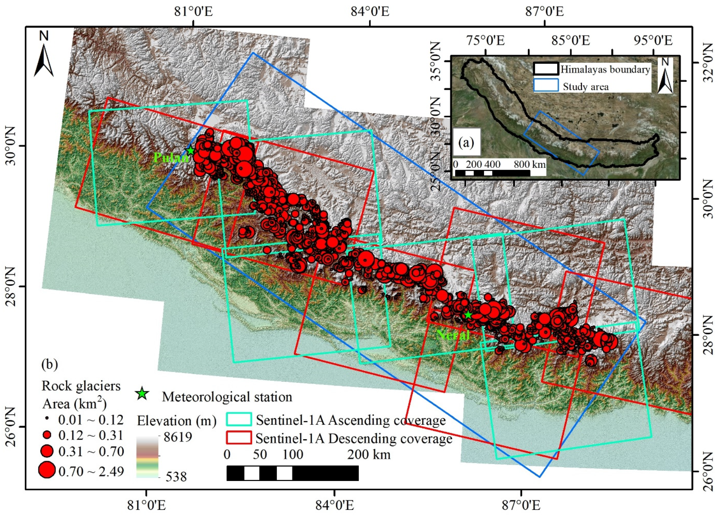
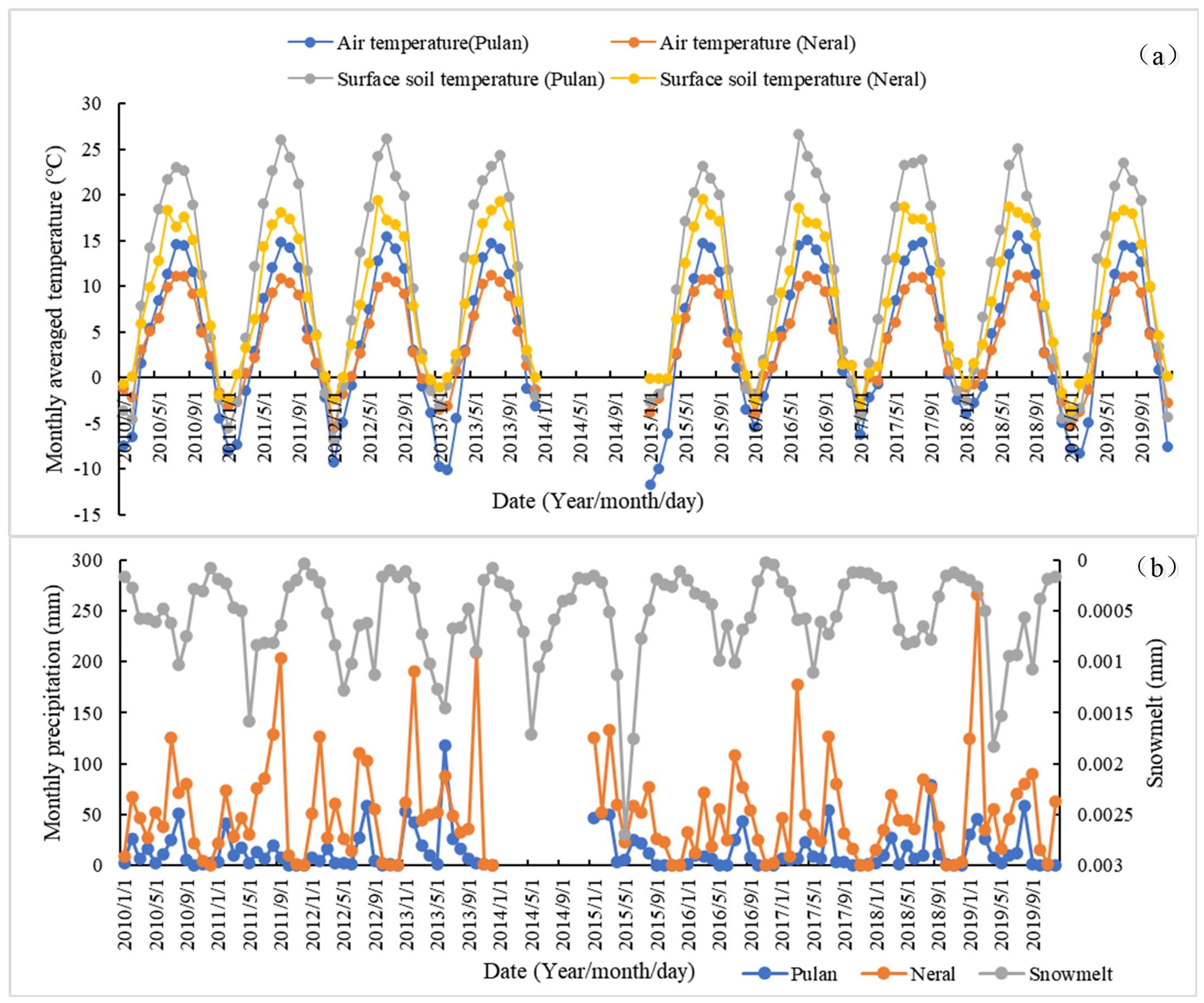
2.1. Study Area

The study area is in the central Himalayas (longitude: 80.74–88.44, latitude: 27.34–30.57) (Figure 1), extending from Mapam Yumco Lake (northwest of the study area) to Kangchenjunga Conservation Area (southeast of the study area). The total area covers 106,403 km². Most of the study area is characterized by continuous permafrost-related periglacial landforms with highly rugged terrain [56]. Altitude ranges from 538 m to 8619 m.

The climate type of the central Himalayas ranges from subtropical in the south to arctic in the north [56]. According to the monthly precipitation and soil temperature data at two meteorological stations (Pulan and Neral) within the study area (Figure 1), the monthly averaged soil temperature ranges from −13 °C to 26 °C through a year (Figure 2a). There is relative low precipitation in October–May; rainfall is mainly concentrated during the summer months (June–September) (Figure 2b). Comparison of Pulan and Neral meteorological characteristics, the soil temperature, and precipitation shows a considerable spatial variation (Figure 2b). The accumulated amount of water that has melted from the snow in the snow-covered area from the ERA-Interim reanalysis data [57] (Figure 2b) indicates that snowmelt oscillates from May to August. Snowmelt is one of the most important factors that influences the penetration and scattering mechanism of the SAR signal [47]. The interferometry coherence between dry or no snow and wet snow is low during the snowmelt oscillations period.

Rock glaciers are widely distributed in the central Himalayas [58]. Following the baseline concepts and practical guidelines of the IPA Action Group rock glacier inventories and kinematics (version 4.1), we visually identified rock glaciers by referring to high-resolution satellite images and manually delineated the outline of each rock glacier. In our study, mandatory criteria of a rock glacier were discernible frontal and lateral margins overriding the surrounding terrain [59]. Multiple sources of satellite images, i.e., Bing Maps, Google Earth, and ESRI satellite maps, were adopted to avoid imagery quality issues that are commonly seen in the region due to the complex terrain and atmospheric conditions. A total of 4962 rock glaciers were identified in the central Himalayas (Figure 1). Based on this dataset, the temporal–spatial coherence of the rock glaciers was calculated to assist the selection of interferogram pairs. The deformation of each rock glacier in the study area was detected using the proposed MT-InSAR method. Most rock glaciers tend to have an aspect of 270~360° and 30~90° (Figure 3a). Due to poor InSAR displacement sensitivity in the south or north component, aspect data can help evaluate deformations. From the point of view of slopes, rock glaciers are widely developed at slopes from 8° to 35° (Figure 3b,c). In some rock glaciers, the local slope exceeds 40° (Figure 3d). Rock glaciers are mainly distributed at altitudes between 3800~6000 m (Figure 3e). The maximum area of an individual rock glacier is less than 2.5 km²; about 4860 rock glaciers have areas of less than 0.5 km² (Figure 3f).

2.2. Datasets

To investigate in detail the large-scale deformations of rock glaciers in the central Himalayas, the MT-InSAR method was applied to interferometric wide swath mode (IW) Sentinel-1A data from both ascending and descending orbits. A total of 12 tracks of ascending and descending data overlapping the rock glacier distribution were processed for this paper (Figure 1,

Table 1. Sentinel-1 data list used in the study area.

Path	Frame	Temporal Span (y/m/d)	Image Counts	Orbit Geometry	Counts of Interferometric Combination
56	93	2018/5/9–2019/1/4	21	Ascending	48
158	92	2018/5/16–2018/12/30	19	Ascending	50
158	87	2018/5/16–2018/12/30	20	Ascending	51
85	88	2018/5/11–2018/12/29	19	Ascending	52
12	84	2018/5/18–2019/1/1	19	Ascending	53
12	89	2018/5/6–2018/12/20	19	Ascending	50
165	493	2018/5/5–2019/1/12	19	Descending	50
92	494	2018/5/12–2019/1/7	19	Descending	50
19	498	2018/5/7–2019/1/2	20	Descending	40
121	496	2018/5/14–2018/12/28	19	Descending	45
121	501	2018/5/14–2018/12/28	19	Descending	46
48	499	2018/5/9–2019/1/16	19	Descending	44

).

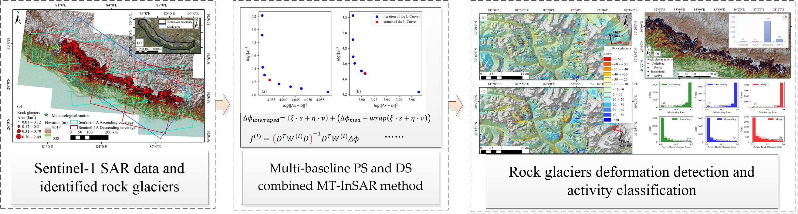
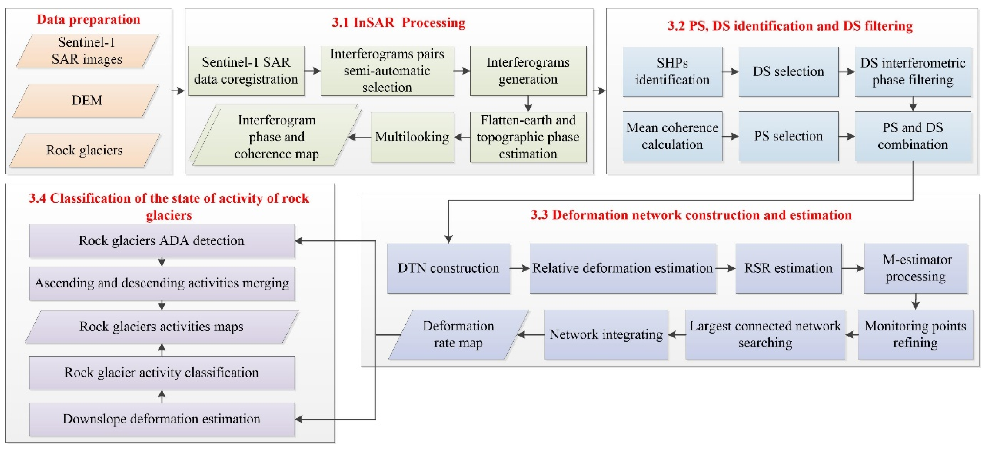
3. Methodology

A multi-baseline PS and DS network-based MT-InSAR method was designed to detect the line-of-sight (LOS) deformation of rock glaciers on a large scale over the central Himalayas using ascending and descending Sentinel-1A SAR data. Rock glacier activity was classified based on multi-geometric LOS deformation estimates. Large-scale deformations and activity characteristics were finally analyzed. The overall processing chain is shown in Figure 4.

3.1. InSAR Processing

Sentinel-1 SAR data coregistration preprocessing, including data extraction, terrain observation with progressive scans (TOPS) splits and de-ramp, geometric coregistration, enhanced spectral diversity (ESD) fine coregistration, re-ramp, burst, and sub-swath merging [53,60], were applied according to the requirements [61].

In the central Himalayas, the rock glacier surface experiences dynamic snowmelt changes, which result in dramatic temporal decorrelation, especially from April to May. Thus, a multi-baseline strategy was adopted to generate the interferograms [62]. A semi-automatic selection of optimum image pairs based on interferometric coherence was adopted [63]. The coherences of all possible interferogram combinations in rock glacier surfaces were generated. The interferograms with rock glacier mean coherence > 0.7 were selected for further processing. After the interferograms generation and selection, the 30 m resolution (1-arcsecond grid) Shuttle Radar Topography Mission (SRTM) digital elevation model (DEM) was used to remove the flat-earth and topographic phase from the original interferograms [61,64]. To improve the signal-to-noise ratio of the interferogram phase and amplitude, all the interferograms were multi-looked by factors of 8 in the range and 2 in the azimuth direction.

3.2. PS, DS Identification, and DS Filter

After the generation of differential interferograms, the deformation parameters were retrieved based on stable scatterers. The scatterers with mean coherence amplitude of all the selected interferograms greater than 0.7 were selected as PS. As observed, the PSs were insufficient over the rock glacier surface. To improve the quality of the interferometric phase and the density of the rock glaciers’ coherent pixels, the DSs were also selected for deformation estimation. The DS objects are statistically homogeneous pixels (SHP) with the same scatter behavior over bare soil, sparse vegetation, or snow-covered surfaces [50,65]. For the SHP identification, the amplitudes of the SAR images were first determined by simple relative amplitude equalization [66,67]. Then, the Anderson–Darling (AD) test was performed to define the SHPs [68,69]. The pixels with SHP count greater than a certain threshold (A 15 × 15 moving window centered around each DS candidate [70] and the number of SHPs greater than 40 [71]) were defined as DS candidates. After the DS candidates selection, the interferometric phase and coherence amplitude of the DS candidates were filtered adaptively using the SHP information [65,70,72]. To reduce the error caused by SHPs with low coherence in simple mean filtering, the coherence between central pixel (DS candidates) and SHPs was used as the weight to filter the interferometric phase [71]. The coherence weight filter is defined as follows:

$${\sigma }_{DS}=\frac{{\sum }_{i=1}^{N}Co{h}_i·{\sigma }_i}{N}$$

(1)

in which ${\sigma }_{DS}$ is the filtered interferometric phase of DS candidates,${\sigma }_i$ is the interferometric phase of SHPs, $N$ is the counts of SHPs, $Co{h}_i$ is the mean coherence of the time-series SAR images between the central pixel and the SHP.

The layover or shadowing effects induced by the SAR geometry may affect the DS selection and the precision of the deformation parameters estimates, which should be simulated and eliminated before the DS selection.

3.3. Deformation Network Construction and Estimation

After the PSs and DSs were identified, a Delaunay triangular network (DTN) was constructed to connect the selected high-coherence scatterers (PSs and DSs). The phase differences of the selected interferograms between two selected highly coherent scatterers at the edge of the DTN was constructed using the phase model described in [35,61,73].

Before parameter estimation, the long arcs with a spatial distance longer than 400 m were rejected due to the significant difference in the atmospheric phase screen (APS) [66]. With the assumption that two adjacent connected scatterers in the DTN have the same APS, the APS was removed by subtracting the phase from the end to the start of the scatterer. The relative deformation rate and DEM error parameters at the arcs of the DTN were estimated by maximizing the absolute value of the temporal coherence [61,62,72]. The optimal relative deformation rate and the elevation error parameters were estimated using the local search Nelder–Mead algorithm [74,75,76].

To evaluate the APS calibration effect and the quality of the relative estimates for all arcs in the DTN, a residue-to-signal ratio (RSR) estimator initially used to detect PS in SAR tomography was modified to evaluate the matching degree between the measurements and the estimated phase [74]. The modified RSR is calculated by the following equation:

$$RSR=\frac{{\sum }_{n=1}^N({\left(A_1^n·A_2^n\right)}^2\left(1-\cos \left(\left|\mathsf{\Delta }{\varphi }_{mea}^n-\mathsf{\Delta }{\varphi }_{est}^n\right|\right)\right))}{{\sum }_{n=1}^N{\left(A_1^n·A_2^n\right)}^2}$$

(2)

where $N$ is the number of interferograms, $A_1^n$ and $A_2^n$ are the coherence coefficients of the starting and ending points of the nth interferograms, $\mathsf{\Delta }{\varphi }_{mea}^n$ is the nth-measured interferometric phase difference, $\mathsf{\Delta }{\varphi }_{est}^n$ is the kth-measured interferometric phase difference acquired from. The lower RSR value implies a better removal of APS and fine estimation of relative deformation parameters. In this paper, the RSRs with a threshold greater than 0.3 indicate ineffectively calibrated APS or an inaccurate estimation of the relative deformation parameters. For those arcs, an M-estimator method was adopted to improve the accuracy of the parameter estimation [66,69].

In the M-estimator process, the temporal phase unwrapping was first conducted based on preliminary estimates results and measured phase:

$$\Delta {\varphi }_{unwraped}=\left(\xi ·s+\eta ·v\right)+\left(\Delta {\varphi }_{mea}-wrap\left(\xi ·s+\eta ·v\right)\right)$$

(3)

where $\xi =2\frac{b_{\perp }}{\lambda R}$, $\eta =2\frac{\Delta t}{\lambda }$, $\Delta t$ is the time span of the interferogram, $s$ and $v$ are the relative deformation rates and the elevation error parameters,$wrap()$ is the wrapping operation. Once all the phases were unwrapped, the relation between the unwrapped phase and relative parameters was reformulated as follows:

$$\mathsf{\Delta }{\varphi }_{unwraped}=DJ=\left[\begin{array}{cc}2\pi {\xi }_1& 2\pi {\eta }_1\\ ⋮& ⋮\\ 2\pi {\xi }_N& 2\pi {\eta }_N\end{array}\right]\left[\begin{array}{c}s\\ v\end{array}\right]$$

(4)

where parameters J can be re-estimated using the least square method. To lower the influence of possible unwrapping phase outliers, parameters J are iteratively solved by assigning smaller weights to significant residual phases.

$$J^{\left(l\right)}={\left(D^T{W}^{\left(l\right)}D\right)}^{-1}{D}^T{W}^{\left(l\right)}\mathsf{\Delta }\varphi$$

(5)

where $l$ is the iteration index and $W$ is the dialog weight matrix; the initial weight matrix ($W^{\left(l = 0\right)}$) was set as the identity matrix and the weight with iteration index l$; W^{\left(l\right)}$ was calculated using the residual phase:

$$r^{\left(l\right)}={\left[r_1^{\left(l\right)},\dots r_N^{\left(l\right)}\right]}^T=\mathsf{\Delta }\varphi -D{J}^{\left(l\right)}$$

(6)

$$w_i^{\left(l+1\right)}=\{\begin{array}{c}1, \mathrm{for} \left|r_i^{\left(l\right)}\right|\le C_{M-estimator}\\ \frac{C_{M-estimator}}{\left|r_i^{\left(l\right)}\right|}, \mathrm{for} \left|r_i^{\left(l\right)}\right|>C_{M-estimator}\end{array}$$

(7)

$$W^{\left(l+1\right)}=diag\left\{w_i^{\left(l+1\right)}\right\}$$

(8)

where C is set to be 1.345 [66], the iteration was terminated on convergence and parameters $J$ were finally determined [66]. After re-estimating the relative parameters by the M-estimator at the arcs with high RSR, the RSR of those arcs was re-calculated. Then, the DTN was adjusted by rejecting unreliable arcs with high RSR.

Once the relative parameters of the reliable arcs were acquired, the absolute deformation and DEM error were retrieved by integrating the relative estimates from the connected network [66]. Due to the rejection of high RSR arcs, isolated small networks may exist in the modified DTN which cannot be adjusted together. The largest connected network was identified by using a deep-first search algorithm. The network adjustment (integration) of the largest connected network can be formulated as follows:

$$\mathsf{\Delta }H = G·S$$

(9)

Assuming that the largest connected network contains $P$ arcs and $Q$ selected stable scatterers, $\mathsf{\Delta }H$ is the estimated relative parameters of all the $P$ arcs, and $G$ is the transformation matrix consisting of −1, 0, and 1, and $S$ is the absolute deformation or DEM error parameters of all the $Q$ selected stable scatterers.

In practice, the transformation matrix may be ill-conditioned, which means that the inversion using least square is not stable. Generally, the ridge-estimator-based weighted least square (WLS) method is commonly used in the inversion [66,74]:

$$S={(G^{T}WG+\sigma I)}^{-1}{G}^{T}WH$$

(10)

where $\sigma$ is the regulation parameter and can be determined by the L-curve method [66,76].

In general, the determination of the L-curve corner in the traditional method requires the eigenvalue decomposition of $G$ and the resolution of the regularization parameter by using the truncated singular value decomposition (TSVD) [75]; this process is time-consuming when the connected network in Equation (10) is large. To overcome this drawback, a faster, alternative method was adopted in our work [76]. This method is based on an iteration optimal estimation of the corner in dispersed L-curve sampling points using the Menger curvature of a circumcircle and golden section search method [76].

We verified the effectiveness of the optimal estimation of the dispersed L-curve corner in a sample region of the descending track (Path 48, Frame 499). As depicted in Figure 5, we located the corners of the L-curve (red point in Figure 5); the optimal regulation parameters for elevation (DEM error) and deformation velocity were found efficiently. The successful selection of the L-Curve corner indirectly demonstrated the validity of the proposed method.

Once the optimal absolute deformation rate and the DEM error parameters were acquired, the deformation time series of the DSs in the line-of-sight (LOS) direction were retrieved through conventional PSI processes [35].

3.4. State of Activity of Rock Glacier Detection

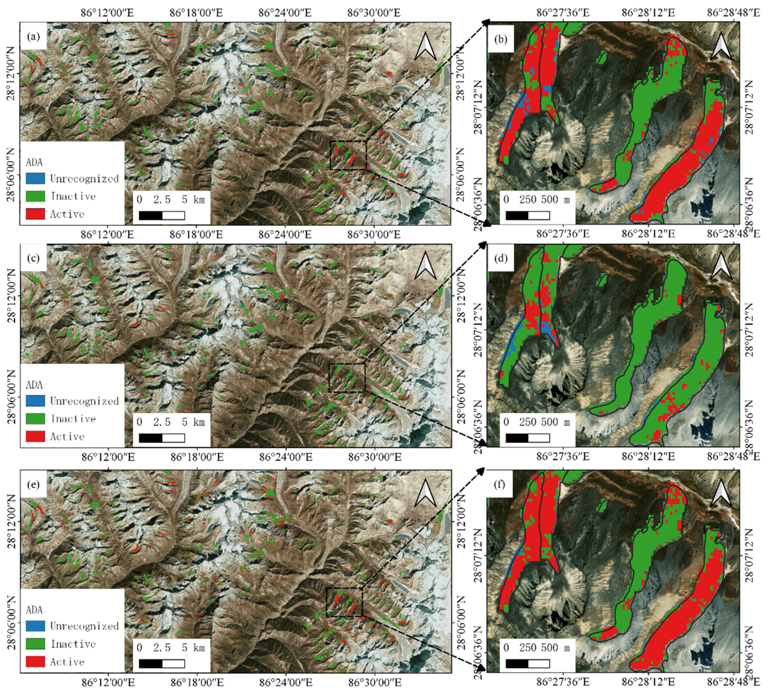
3.4.1. Active Deformation Areas Detection

Active deformation area (ADA) is an effective indicator of displacement measured by MT-InSAR processing [77,78]. Based on the deformation acquired from Section 3.3, ADA was identified using the standard deviation of the deformation map (${\sigma }_{map}$). As the rock glacier outline was identified, a stability threshold of $2{\sigma }_{map}$ was set to discriminate the active points of the rock glacier [78]. Rock glacier activity can be classified into three classes:

$$R{G}_{activity}=\{\begin{array}{c}Unrecognized if v=nan \\ Inactivate if \left|v\right|<2{\sigma }_{map}\\ Activate if \left|v\right|>2{\sigma }_{map}\end{array}$$

(11)

where $\left|v\right|$ is the absolute deformation velocity of the rock glacier monitoring point. $R{G}_{activity}$ is the activity of the rock glacier monitoring point.

In this paper, to improve the monitoring rate of the ADA in the rock glacier surface, the activity of rock glaciers acquired from both ascending and descending deformation was merged:

$$R{G}_{merge}=\{\begin{array}{c}Unrecognized if {RG}_{asc} and {RG}_{des} are Unrecognized\\ Inactivate if {RG}_{asc} and {RG}_{des} are Inactivate\\ Activate if one of the {RG}_{asc} and {RG}_{des} is Activate\end{array}$$

(12)

where $R{G}_{asc}$ and $R{G}_{des}$ are the activities of the rock glacier pixel in the ascending and descending orbit data acquired using Equation (11). $R{G}_{merge}$ is the merged activity.

3.4.2. Rock Glacier Activity Classification

Recently, the IPA Action Group established a baseline concept of rock glacier inventories and kinematics as well as a standard guideline for inventorying regional rock glacier activity using InSAR data [59,79]. Following the baseline concept and the guideline, we further classified the rock glacier activity using the MT-InSAR detecting results. First, the LOS surface velocity of both geometries (ascending and descending) was projected to the direction of the steepest slope using the method proposed by Notti et al. [49]. Second, the median downslope deformation velocities of all of the valid pixels within the extent of each rock glacier were calculated [44]. Finally, the mean of both downslope velocities derived from the ascending and descending observations was calculated as the final downslope deformation velocity [44]. The kinematic attribute was assigned according to the rules defined in the guideline [59], and all of the identified rock glaciers were classified into four categories of activity, i.e., undefined, active, transitional, and relict [59].

4. Results

We applied the proposed MT-InSAR method to all 12 tracks of Sentinel-1 data covering all identified rock glaciers (Table 1, Figure 1). Balancing the effect of numerous monitoring points (>8 million in some tracks) and arcs in DTN to computational efficiency, the selected monitoring points were segmented into several subsets (a maximum of 3 million points in each segmentation was allowed in this study). The DTN was constructed, and the relative parameters of the reliable arcs in each segmentation were acquired. Selecting stable reference points in each segmentation network is critical for integrating the relative estimates to absolute deformation rate and the DEM error (Equation (10)). We set all reference points manually using mean interferometric coherence and high resolution Bing optical images, and the candidate point with high coherence (>0.9) and distributed in the mountain bedrock region was selected [55,80]. Once the reference points were determined, the ridge-estimator-based WLR was performed to acquire the absolute deformation velocity and DEM error. Finally, we merged the deformation velocities of all segmentations and tracks by calculating the datum offset with the analysis of the distribution of the homonymous point difference of the subset and multitrack overlapping areas [81].

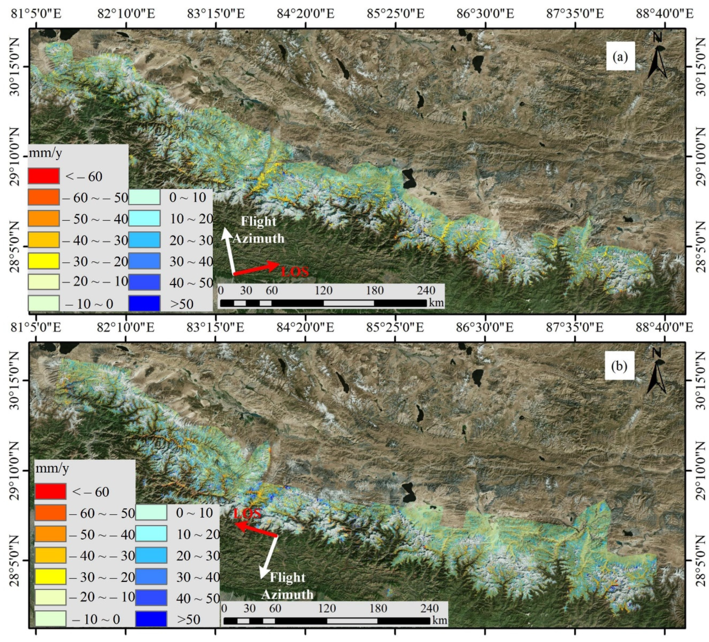
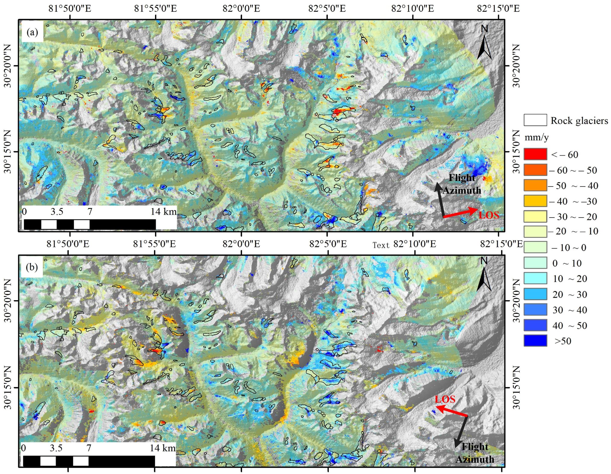
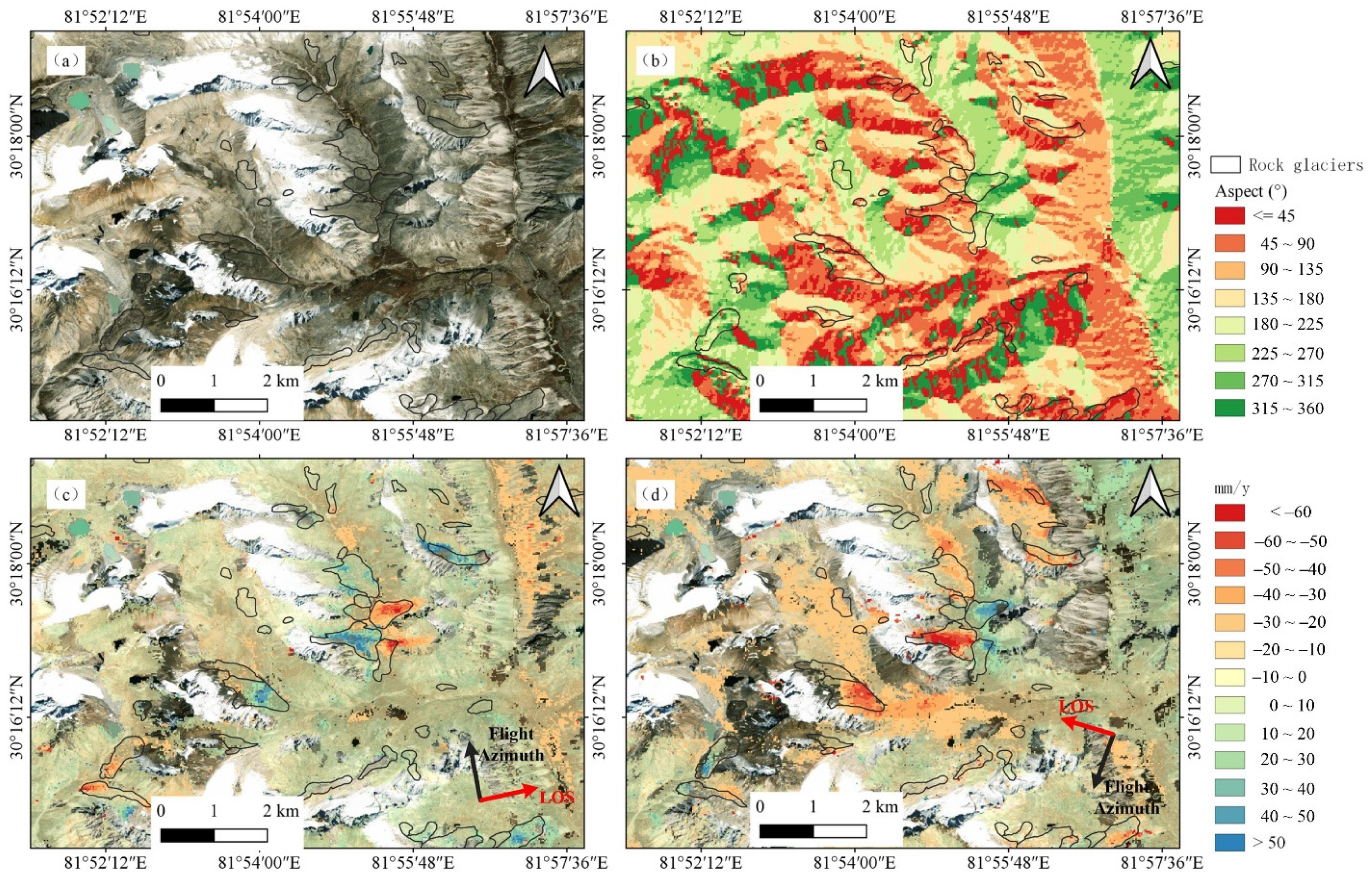
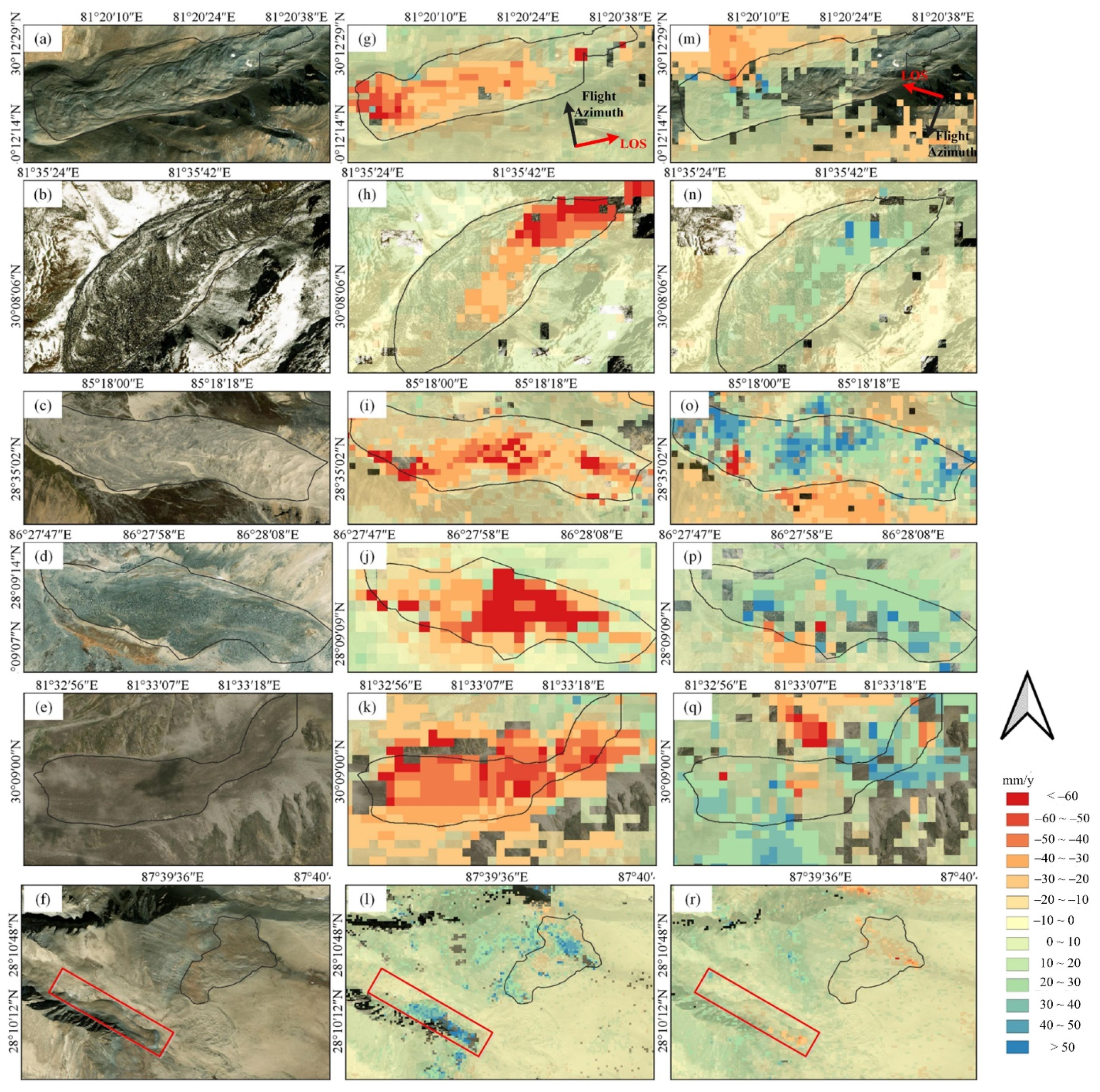
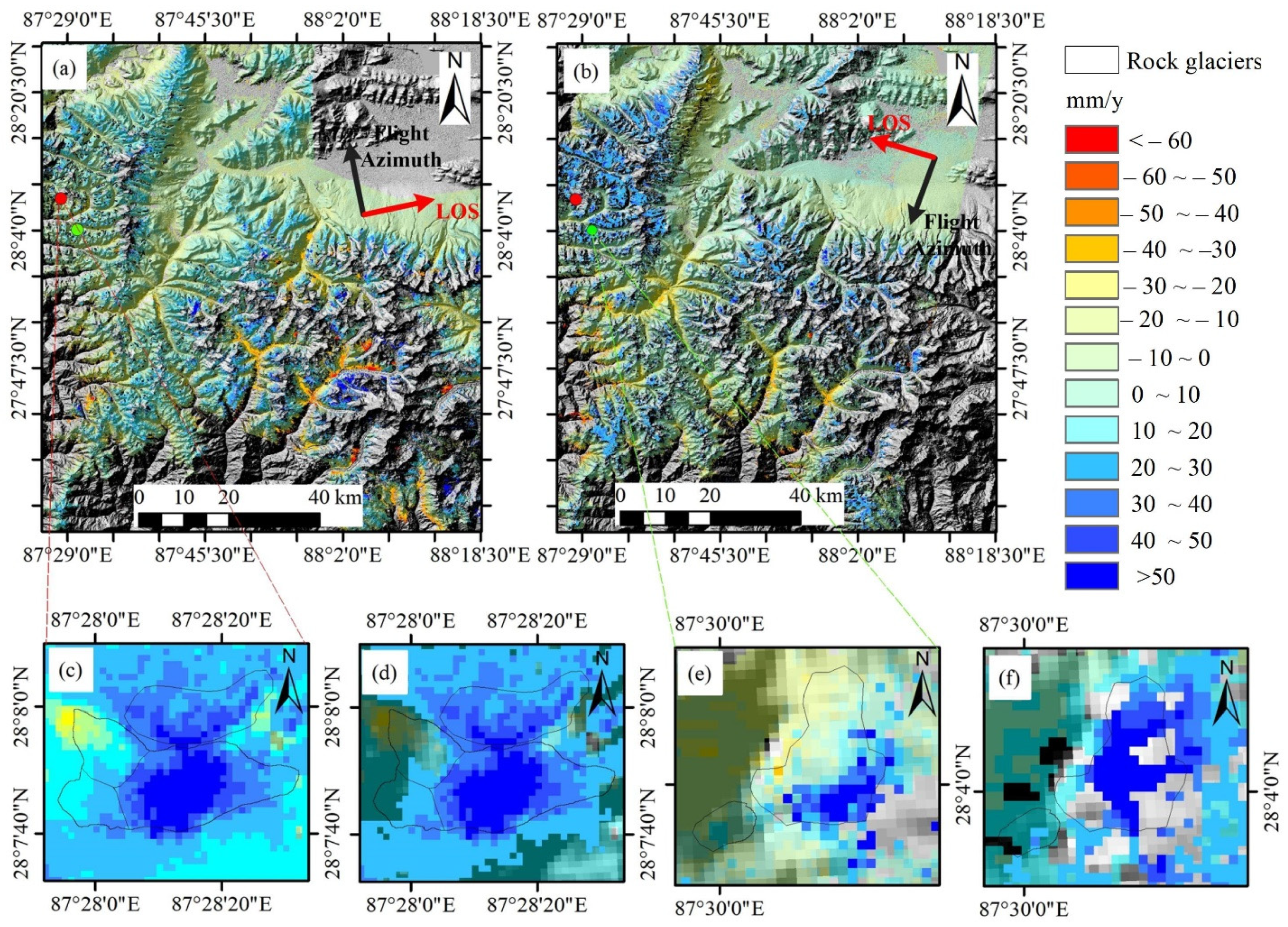
4.1. Deformation Rates over the Central Himalayas

Based on the processing chain mentioned above (Figure 4), the deformation velocities of rock glaciers and their surrounding areas in the LOS direction were obtained from the Sentinel-1A ascending and descending geometries. We observed LOS deformation velocities in the central Himalayas ranging from −150 to approximately 150 mm (Figure 6). The deformation velocity standard deviations of ascending data and descending data were 14.42 and 14.74 mm/y, respectively. The deformation velocities of permafrost showed lower variations compared with rock glacier landforms (Figure 7).

As shown in the randomly selected zoom-ins in Figure 7, the deformation anomalies of active rock glaciers were observed both in ascending and descending geometries. Since the rock glaciers are distributed in high mountain areas, the aspects of rock glaciers show significant spatial heterogeneity (Figure 8b). Generally, a positive deformation rate represents the motion of the ground toward the satellite, and conversely, negative velocities represent the motion away from the satellite [39]. As shown in Figure 8c,d, the deformation rate shows opposite trends in aspects (eastward and westward) and SAR orbits (ascending and descending). Thus, high positive and negative deformation velocities in rock glacier surfaces indicate that the rock glacier is unstable. The discrepancies in the deformation trends in different aspects and SAR orbits demonstrated the effectiveness of our proposed method (Figure 8). Previous studies showed that the aspect facing away from the satellite captured a more significant portion of the actual deformation in the slope direction [40].

Figure 9 shows the detailed deformation of individual rock glaciers in ascending and descending geometries. The active displacements observed from ascending orbit data were notable when the aspect of the rock glacier faced away from the satellite. Thus, the extraction effects of active rock glaciers can be improved by combining the deformation detecting results of both ascending and descending geometries. In general, the activity of rock glaciers is classified based on the morphological characteristics acquired from high-resolution optical images [19] (Figure 9a–f). The rock glacier with unambiguous, complex, and extensive ridge and swale flow banding indicates high activity [19]. However, based on the criterion provided in [19], a rock glacier classified as inactive by optical images (Figure 9e,f) shows deformation velocity greater than 60 mm in its moving area and reveals obvious deformation compared with its surrounding areas (Figure 9k,l). Thus, the deformation acquired from the MT-InSAR method provides a quantitative indicator for the classification of the regional activity of rock glaciers. An unrecognized rock glacier (red block in Figure 9f) shows high deformation velocities both in ascending and descending geometries (Figure 9l,r). Thus, the deformation information can provide an additional indicator for rock glacier recognition.

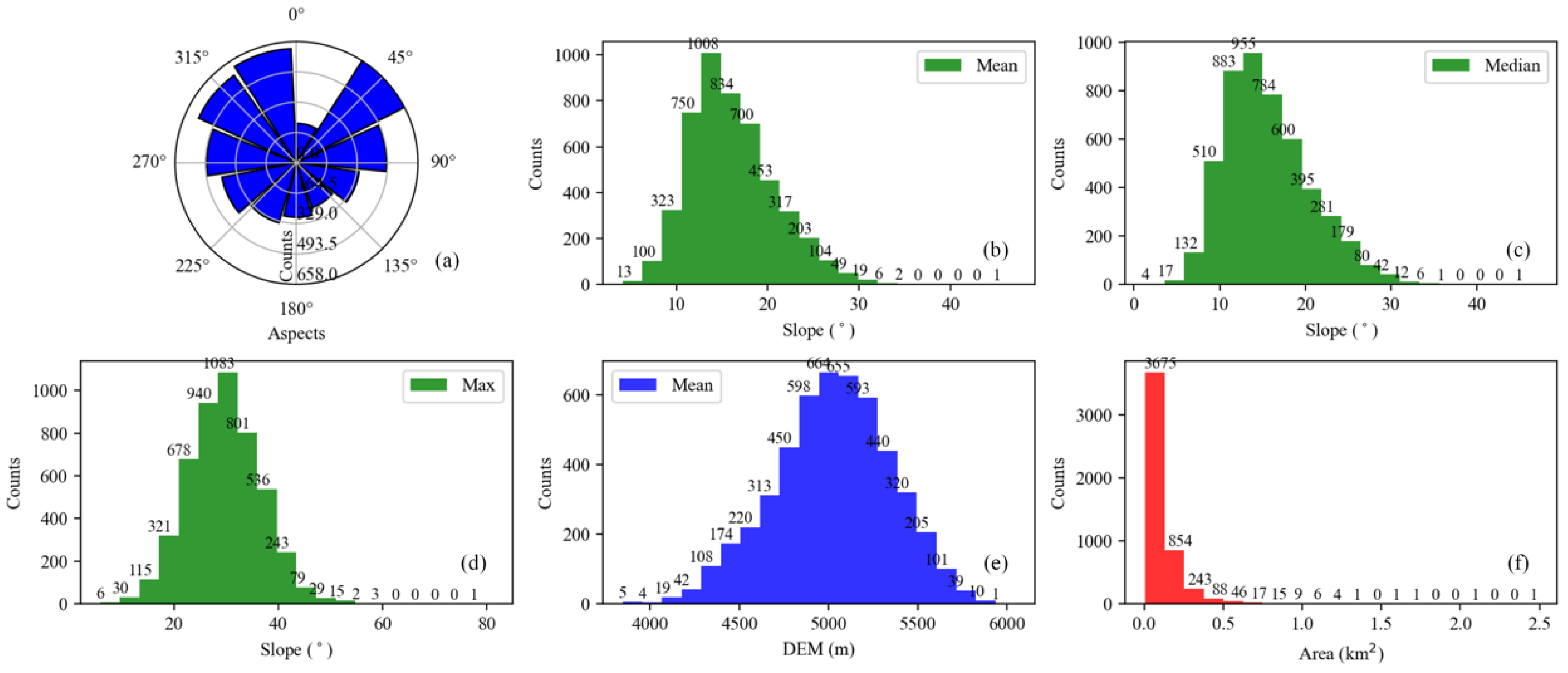
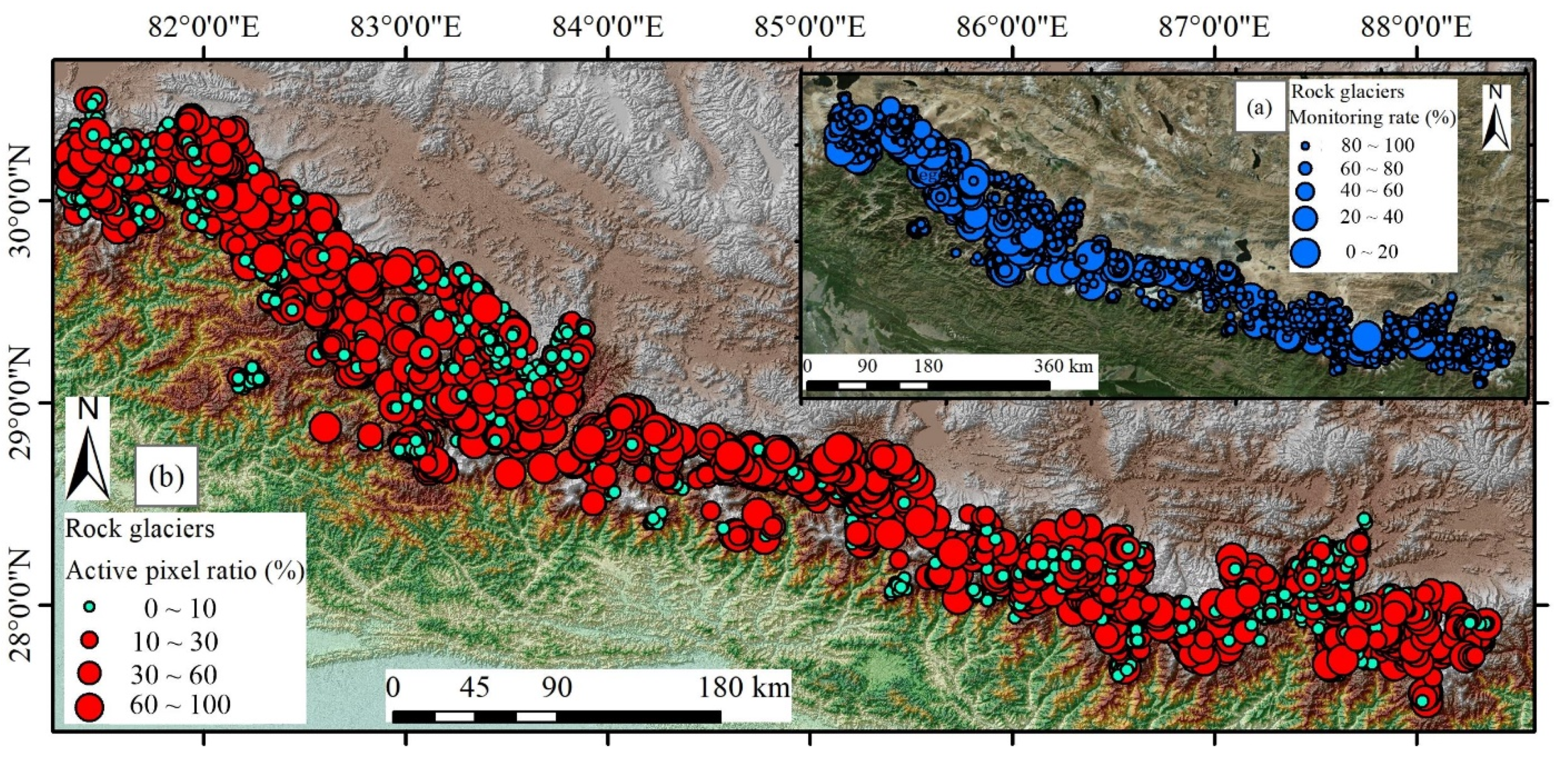
4.2. Rock Glacier Activity Statistical Analysis

4.2.1. Rock Glacier ADA

According to the recognition of the rock glaciers over the central Himalayas (Figure 1), the mean, median, maximum, and the difference between the maximum and minimum deformation of 4962 rock glaciers were calculated (Figure 10). As shown in Figure 10a,b,e,f, the mean and median displacement rate ranged from 0 to 75 mm/y both in ascending and descending orbits; these distributions also revealed the proportion of the moving area within the outline of each rock glacier. Considerable diversity of deformation velocity was reported among the rock glaciers due to the variation in deformation velocity of the intact rock glaciers and the existence of relict rock glaciers in the identified rock glaciers. More than half of the rock glaciers have large deformation points or zones (>3200 in ascending estimates and >2800 in descending estimates) (Figure 10c,d,g,h). About 60% of the rock glaciers show great spatial displacements variation, with deformation differences of over 40 mm/y (Figure 10d,h). In general, the deformation velocity of a rock glacier unit often shows spatial heterogeneity to a certain degree due to the diversities of the internal structure and terrain slope [59]. Consistent with the IPA Action Group Rock glacier inventories and kinematics guideline, the deformation difference between the terminal part (front) lateral margins, rooting zone, and the central part of a rock glacier was also found in this study (Figure 9g–j).

To evaluate the activity of rock glaciers from the MT-InSAR deformation estimation results, active thresholds with 28.84 mm/y in the ascending orbit and 29.47 mm/y in the descending orbit were established using the standard deviation of the deformation map ($2{\sigma }_{map}$). The ADA of all rock glaciers was calculated based on the methodology explained in Section 3.4.1 (Figure 11).

Figure 12 shows an example of ADA extraction results at different zoom-in scales. The ADA extracted from the ascending geometry was consistent with the descending geometry in most rock glacier surfaces. At the same time, diversity in the proportion of ADA existed in some rock glaciers (Figure 12d,e). The reason for this is that the deformation signal cannot be well detected when the rock glacier aspects face toward the SAR LOS azimuth [39]. In addition, several tracks of SAR data were included in the study area. The individual reference point in every sub-region needs to be selected individually. When the reference points are chosen in the active (large deformation) region, there will be a certain estimation error and deformation difference between ascending and descending results [55].

As shown in Figure 12a,c, in some pixels of individual rock glaciers, ADA was undetected due to decorrelation; the overall activity state of an individual rock glacier was unrepresentative when there was a small proportion of monitorable pixels. As seen in Figure 13a,b, about 4646 rock glaciers in the ascending orbit and 4502 in the descending orbit were classified with more than 50% of monitored pixels. The final merged ADA map of the rock glaciers in the central Himalayas was obtained based on Equation (12) (Figure 11 and Figure 12e,f). As shown in Figure 13c, the monitoring rate was significantly improved; about 4327 rock glaciers were monitored with a monitoring rate of over 90% (Figure 13c).

According to the ADA classification results (Figure 11 and Figure 12) and monitoring rate statistics (Figure 13a–c), the proportion of active pixels in all monitorable pixels (active pixels ratio) was counted (Figure 13d–f). Considering the balance between monitoring rate and the representativeness of the ADA to individual rock glaciers, the rock glacier active ratios for a monitoring rate greater than 30% were calculated (Figure 11 and Figure 13d–f,

Table 2. Active rock glacier statistics in the central Himalayas.

Indicators	Ascending		Descending		Merged
	Counts	Percentage (%)	Counts	Percentage (%)	Counts	Percentage (%)
Mean > 2σ	492	11	582	12	933	19
Median deformation > 2σ	414	8	504	10	775	16
Maximum deformation > 2σ	2757	59	2817	60	3538	71
Active rock glacier ratios > 0.1 and Monitoring rate > 0.3	1589	32	1588	32	2446	49

). As shown in Figure 13d,e, a total of 3034 rock glaciers in ascending and 3079 rock glaciers in the descending orbits are in a low activity ratio. After merging the geometries, the active rock glacier ratios increased from 32% to 49% (Figure 13f).

Table 2 summarizes the statistically highly active rock glaciers corresponding to different analysis indicators (mean, median, maximum deformation, and active rock glacier ratios). The ascending and descending merged mean and median deformation greater than 2σ were about 19% and 16%, respectively (Table 2). These results indicate that only a small part of the rock glaciers was in an active state, while about 71% of rock glaciers showed high local activity (maximum deformation greater than 2σ) (Table 2). Thus, binary classification of the activity of a rock glacier (active or inactive) cannot be based just on the indicators of mean and median deformation. The statistics of rock glaciers with a monitoring rate greater than 30% and active rock glacier ratios greater than 10% were calculated and more detailed characterizations of rock glaciers were acquired. The statistical results show that 49% of rock glaciers were active (Table 2).

4.2.2. Rock Glacier Activity

Based on the rock glacier activity classification strategy mentioned in Section 3.4.2, the downslope deformation rate of the recognized 4962 rock glaciers in the study area was acquired by LOS surface velocity downslope projection and merging ascending and descending downslope deformation results. Figure 14a,b shows that the mean and median downslope displacement rate was below 300 mm/y. Similar to the LOS deformation estimates (Figure 10c,d,g,h), rock glaciers showed large spatial inside displacements variation (Figure 14e), and the moving area existed in 42% of the studied rock glaciers (Figure 14d).

Based on the rock glacier inventory conducted in the previous study [44], the median of rock glacier pixels was determined to represent the rock glacier kinematic attribute (Figure 14b). Following the IPA Action Group guidelines, rock glaciers with a surface velocity of <10 mm/y were considered relict, 10–100 mm/y were considered transitional, and faster rock glaciers were considered active [59]. The activity of rock glaciers distributed in the study was acquired (Figure 15a). The rock glaciers with a monitoring rate of less than 30% were classified as undefined. As shown in Figure 15b, transitional rock glaciers represented 86% of the inventory; 12% were active.

5. Discussion

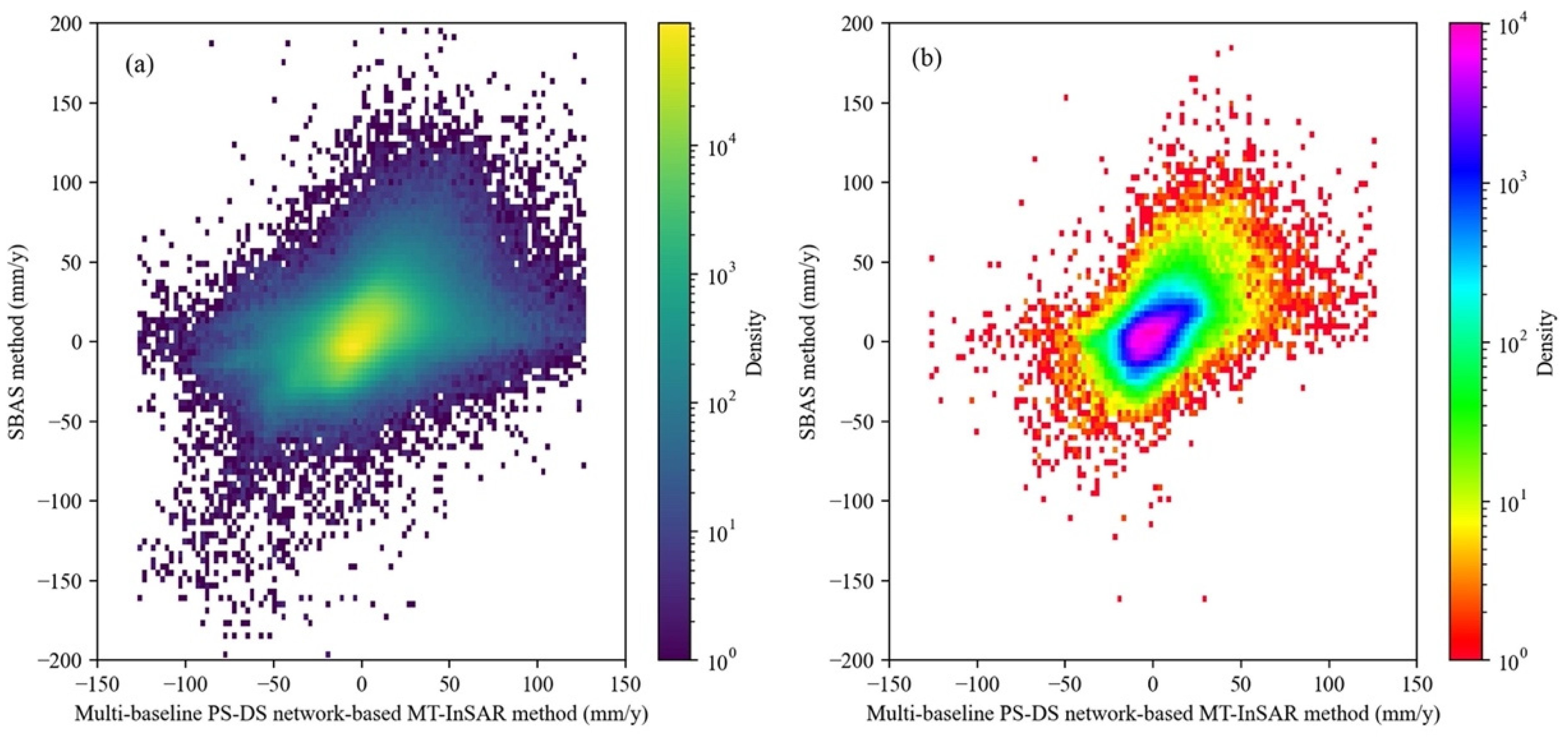
5.1. Cross Comparison between the Proposed MT-InSAR Method and the SBAS Method

We evaluated the consistency of the deformation rate derived from the multi-baseline PS–DS network-based MT-InSAR method and the SBAS method [80] in a sample region of the descending track for Path 48, Frame 499 (Figure 16). As shown in Figure 16, the deformation rates show similar spatial distributions, although heterogeneities exist in some regions. In some rock glaciers, active deformation was acquired by both methods (Figure 16c–f). Figure 16e,f indicates that a higher monitoring rate was achieved by the proposed MT-InSAR method, likely because coherence weight filtering was performed for selected DS and the quality of the interferogram phase was improved. On the other hand, the conversion from phase to displacement time series was performed by minimizing the interferometric phase residual in the SBAS method [80]. When critical interferometric links are missed in low interferometric coherence pairs there will be no displacement estimates [82]. As shown in Figure 16a,b, the area outside of rock glaciers also shows LOS deformation as high as 60 mm/y. After visual investigation, we found that most of deformations were likely due to periglacial talus deformation or permafrost seasonal thaw subsidence, and we believe that the presented method could be helpful for detecting the deformation activity of the talus.

Figure 17 shows the density scatter plots between the two methods for the overall sample region and the rock glacier area. Compared with the entire area of the sample region, a higher density correlation was found in the rock glacier surface. The results reveal that both the proposed MT-InSAR and the SBAS method were able to detect the activity of the rock glaciers. In the high mountain region, the multi-baseline PS–DS network-based MT-InSAR approach shows an advantage compared with the SBAS method. In the SBAS method, the tropospheric delay correction was performed using the global atmospheric model (GAM) [53] or the empirical relationship between the stratified tropospheric delay and topography [83]. The interferograms in the high relief region are often strongly affected by a delay correlated with topography [84]. It is difficult to simulate the relationship between vertical stratification and topography using the empirical model (linear or power-law) and GAM on a large scale in the periglacial zones of the Himalayas [55]. However, the DTN network was constructed to connect the coherence points with similar APS in the PS–DS network-based MT-InSAR method. The arcs with large APS variations were rejected. In addition, the deformation parameter estimation error caused by topographic-correlated atmospheric delay was reduced by RSR and the M-estimator method. The SBAS method in MintPy does not use the temporal deformation model in the network inversion [80], which is more suitable for estimating deformation in low relief permafrost regions.

5.2. Comparison with Other Rock Glacier Surface Displacement Studies

It was extremely difficult to validate the deformation monitoring results with TSL or GPS, as no such data were available to this study [44]. To evaluate the reliability of our results, the deformation characteristics of rock glaciers estimated by InSAR and MT-InSAR in previous studies were compared (Table 3). Due to its merits, many studies have used InSAR to retrieve surface deformation information of rock glacier landforms in periglacial environments such as Tien Shan, the Alps, and the Himalayas. The studies listed in Table 3 indicate that the rock glacier deformations show large variations (<2000 mm). The displacement velocities in the central Himalayas estimated using the MT-InSAR method are slightly lower than those derived from the conventional DInSAR technique [27,44]. This difference was likely due to the fact that the relative deformation estimated with the DInSAR method is based on a short time interval, which is not susceptible to the influence of deformation decorrelation [27]. The PSI or SBAS methods are more suitable for observing slow slope movements of rock glaciers at the mm/y scale [32]. Compared with the estimation results acquired using the SBAS or PSI method, a similar deformation variation range was acquired in this study (Table 3). Dini et al. described the deformation mapping of hundreds of rock glaciers in the Himalayas of northwestern Bhutan. The velocity in the LOS is around 100 mm/y, which is similar to our results [43]. Eike et al. classified 1433 rock glaciers over the Nyainqêntanglha using the MT-InSAR method, finding that about 18.5% of rock glaciers were active with higher median surface velocities of up to 87 cm/y (direction of the steepest slope) [44] (Table 3). Compared with the median deformation results acquired in our study (Table 2), the percentage of reported active rock glaciers (12%) was lower than that of Eike et al. [44]. However, the highly active rock glacier ratio was acquired using a threshold of active rock glacier ratio > 0.1 and monitoring rate > 0.3 (Figure 13 and Table 2).

The 75th percentile downslope velocity was another effective indicator used to represent the total deformation velocity of a rock glacier in a recent study [85]. With this indicator, about 4700 rock glaciers showed downslope deformation greater than 100 mm/y (Figure 14c), reporting more active rock glaciers. If the 75th percentile represents the rock glacier downslope deformation, the active rock glaciers will increase to 30%. As introduced in the IPA Action Group, the transitional rock glaciers can either evolve towards a relict (degraded) or an active state [59]. In this study, the observation time window was shorter than one year, and some active rock glaciers may have been classified as transitional due to incomplete representation of the activity status. The accuracy of deformation detection could be further improved by measuring the deformation using observations acquired over multiple years to reduce potential inter-annual variations for rock glacier deformation [59] (Figure 15).

Table 3. Rock glacier deformation monitoring using InSAR and MT-InSAR methods in previous studies.

Study Area	Observation Period	SAR Dataset	Method	Deformation Rate (mm/y)	Deformation Direction	Authors
Southern Dry Andes	2014–2016	Sentinel-1	InSAR	22–1700	LOS	[17]
Sierra Nevada	2007–2008	ALOS PALSAR	InSAR	550	Slope	[4]
Northern Tien Shan	2007–2009	ALOS PALSAR	InSAR	50	Slope	[31]
Northern Tien Shan	1998–2018	ALOS PALSAR, Sentinel-1	InSAR	0–1000	LOS	[86]
Swiss Alps	2008–2017	TerraSAR-X, Sentinel-1	InSAR	0–2000	LOS, Slope	[33]
Western Swiss Alps	2008–2012	TerraSAR-X	PSI, SBAS	<35 for PSI And 350 for SBAS	LOS	[32]
Nyaiqêntanglha Range, Tibetan Plateau	2016–2019	Sentinel-1	MT-InSAR	870	Slope	[44]
Himalaya of NW Bhutan	2007–2011	Envisat, ALOS PALSAR	SBAS	100	LOS	[43]
Southern Carpathian Mountains	2007–2010	ALOS PALSAR	SBAS	0–30	LOS	[34]

Table 3. Rock glacier deformation monitoring using InSAR and MT-InSAR methods in previous studies.

Study Area	Observation Period	SAR Dataset	Method	Deformation Rate (mm/y)	Deformation Direction	Authors
Southern Dry Andes	2014–2016	Sentinel-1	InSAR	22–1700	LOS	[17]
Sierra Nevada	2007–2008	ALOS PALSAR	InSAR	550	Slope	[4]
Northern Tien Shan	2007–2009	ALOS PALSAR	InSAR	50	Slope	[31]
Northern Tien Shan	1998–2018	ALOS PALSAR, Sentinel-1	InSAR	0–1000	LOS	[86]
Swiss Alps	2008–2017	TerraSAR-X, Sentinel-1	InSAR	0–2000	LOS, Slope	[33]
Western Swiss Alps	2008–2012	TerraSAR-X	PSI, SBAS	<35 for PSI And 350 for SBAS	LOS	[32]
Nyaiqêntanglha Range, Tibetan Plateau	2016–2019	Sentinel-1	MT-InSAR	870	Slope	[44]
Himalaya of NW Bhutan	2007–2011	Envisat, ALOS PALSAR	SBAS	100	LOS	[43]
Southern Carpathian Mountains	2007–2010	ALOS PALSAR	SBAS	0–30	LOS	[34]

5.3. Source of Rock Glacier Surface Displacements and Activity Estimation Error

The challenges of InSAR displacement monitoring in the Himalayas, such as temporal decorrelation and atmospheric phase screen errors mentioned in the previous study [27], were reduced through the automatic selection of optimum interferometry combination pairs, DS selection and phase optimization, the improvement of the deformation estimation network, and multiple datasets (ascending and descending). The permafrost of the region with rock glaciers undergoes seasonal freezing and thawing that cannot be described correctly by the linear deformation model [45]. The Stefan model or sinusoidal approximation seasonal deformation models have been commonly used to map seasonal variation processes of permafrost [43,45,73]. The applicability of those models was well demonstrated on the local scale [43,45,73]. However, as shown in Figure 2, the soil surface temperature shows significant spatio-temporal variations. It is unreasonable to characterize the physical process of permafrost displacements with a single sinusoidal or the Stefan model. The multivariate Stefan model, which can characterize the deformation process of each monitoring point (PS or DS) needs to be further explored. Considering the temporal range of this study (from May 2018 to January 2019), the deformation process can be modeled in a linear deformation model due to the short temporal span and the relatively uncomplicated thawing and freezing process. It is appropriate to estimate the short-term deformation using a linear deformation model. In the future, the accuracy of deformation estimation results could be further improved after the integration of the multivariate Stefan model into the DTN.

In the cases when the deformation of the rock glacier is facing the SAR incident angle or the deformation is mainly concentrated in the north or south direction, the InSAR monitoring results have insufficient sensitivity, the active deformation is not noticeable, and the ADA estimation rate is underestimated [44]. As shown in Figure 3a, many rock glaciers are distributed in the north or south direction. The influence of the InSAR sensitivity to ADA detection was reduced by integrating ascending and descending geometric deformation monitoring results (Figure 6 and Figure 11).

The deformation decorrelation is another source of error for the underestimation of the monitoring rate and active ratio. In general, the maximum detectable displacement is equal to half the wavelength of the emitting satellite (~2.8 cm for Sentinel-1) in a single interferogram [87]. Due to the satisfactory temporal resolution of Sentinel-1 data (12 days), in this study, most of the interferograms were in temporal baselines shorter than 48 days. The interferograms pairs were selected based on the coherence of rock glaciers. Thus, the deformation decorrelation was reduced. As shown in Figure 7, the deformation decorrelation in some monitoring points of the rock glacier still exists to some extent. The deformation decorrelation of active rock glaciers can be solved by supplementing the deformation estimation using the offset tracking method in the following study [88].

The interferometric decorrelation caused by snowmelt is the principal problem restricting MT-InSAR applications in periglacial regions on long time series and in large scale [29]. With the shorter revisit cycles of Sentinel-1, sufficient interferometric pairs can be acquired after avoiding images with thick snow cover or snowmelt. The long-term monitoring of rock glaciers could be conducted by separating the single annual temporal data into several sub-datasets, and the annual deformation rate and activity can be acquired by integrating the estimation results of each sub-dataset.

5.4. The Advantages of the Multi-Baseline PS–DS Combined MT-InSAR Method

Considering the limitations mentioned in Section 5.3, the proposed MT-InSAR workflow is a suitable choice for monitoring large-scale rock glacier activity. In previous studies, the deformation estimation of rock glaciers was generally conducted with the SBAS method. The multi-baseline PS–DS combined network-based MT-InSAR method was first used in large-scale complex periglacial environments. It provides a new option for deformation monitoring research of rock glaciers when the topography-correlated atmospheric delay cannot be removed effectively and phase unwrap errors exist [55]. In addition, the multi-baseline selection strategy of the SBAS method and DS phase filter method were introduced into the DTN network. The insufficient monitoring points problem of the traditional PSI method was effectively solved. Moreover, the relative and absolute deformation parameters retrieval strategy in the DTN were modified to satisfy the deformation estimation over the periglacial environments with a more powerful and efficient form. Additionally, based on the full mapping of rock glaciers over the central Himalayas (Figure 1 and Figure 3), the deformation characteristics (Figure 7) and activity indicators (Figure 12 and Figure 15) around all rock glacier pixels were detected, providing comprehensive information for large-scale periglacial environment permafrost distribution and landslide disaster studies.

6. Conclusions

In this paper, we presented an application of the MT-InSAR technique with Sentinel-1 ascending and descending geometries data to detect rock glaciers activity in the Himalayas’ periglacial zones. Out of a total of 4962 identified rock glaciers in the central Himalayas, the activity of 4327 rock glaciers was successfully detected. The conclusions are summarized as follows:

(1)

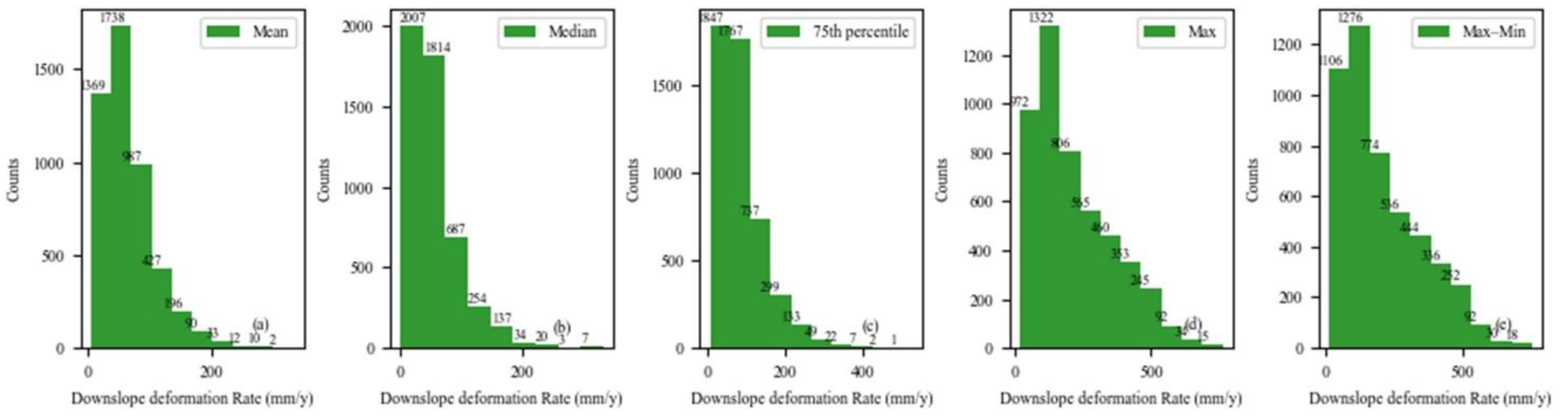
Our analysis shows that the deformation rate of rock glaciers in the central Himalayas is experiencing spatial variations, with velocities ranging from 0 to 75 mm/y. More than half of the pixels of the rock glaciers have large deformations. Noticeable deformation differences between rock glaciers and their surrounding areas were found. The active deformation discrepancies can provide a visual indicator for the recognition of rock glaciers.

(2)

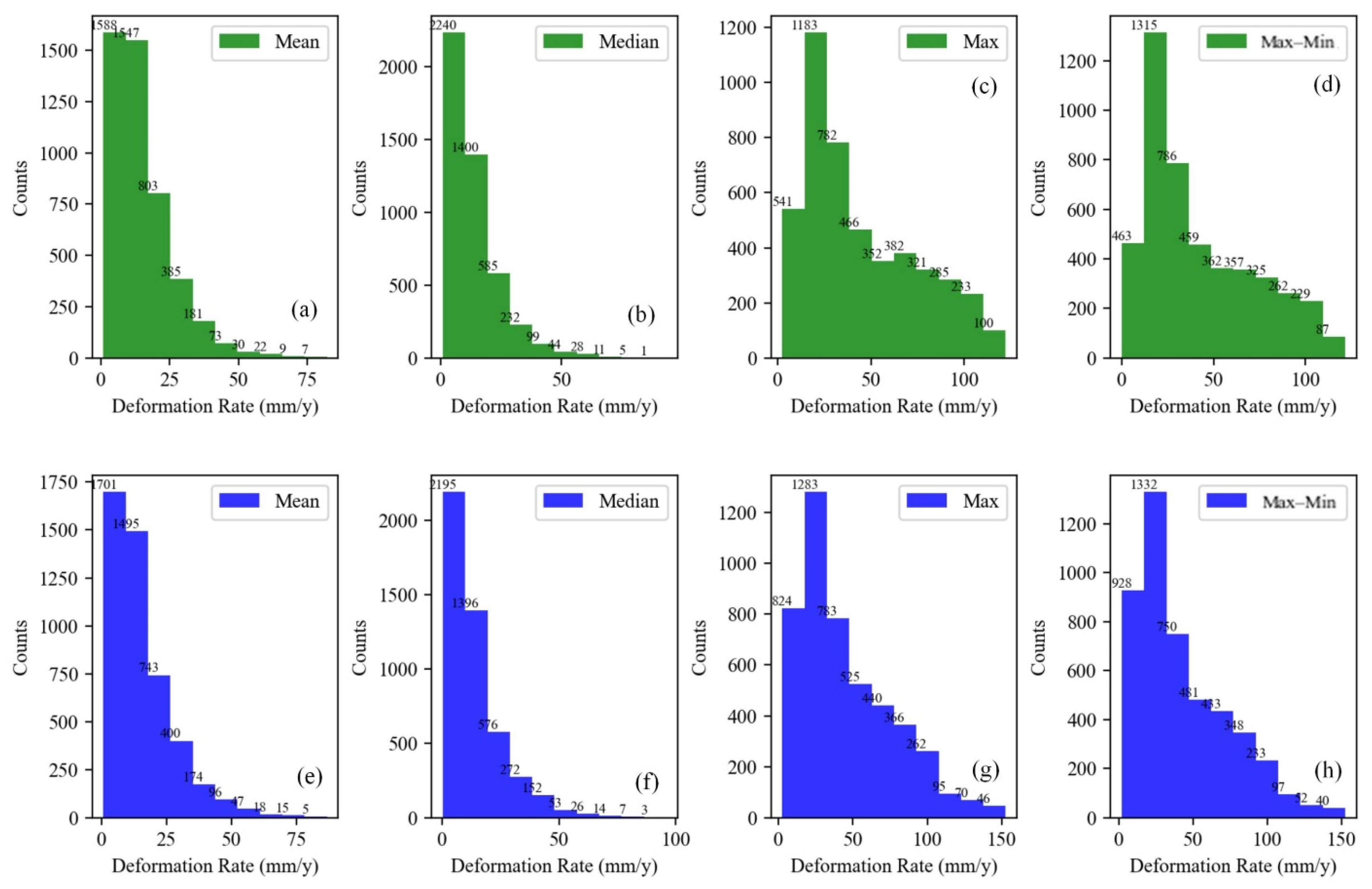
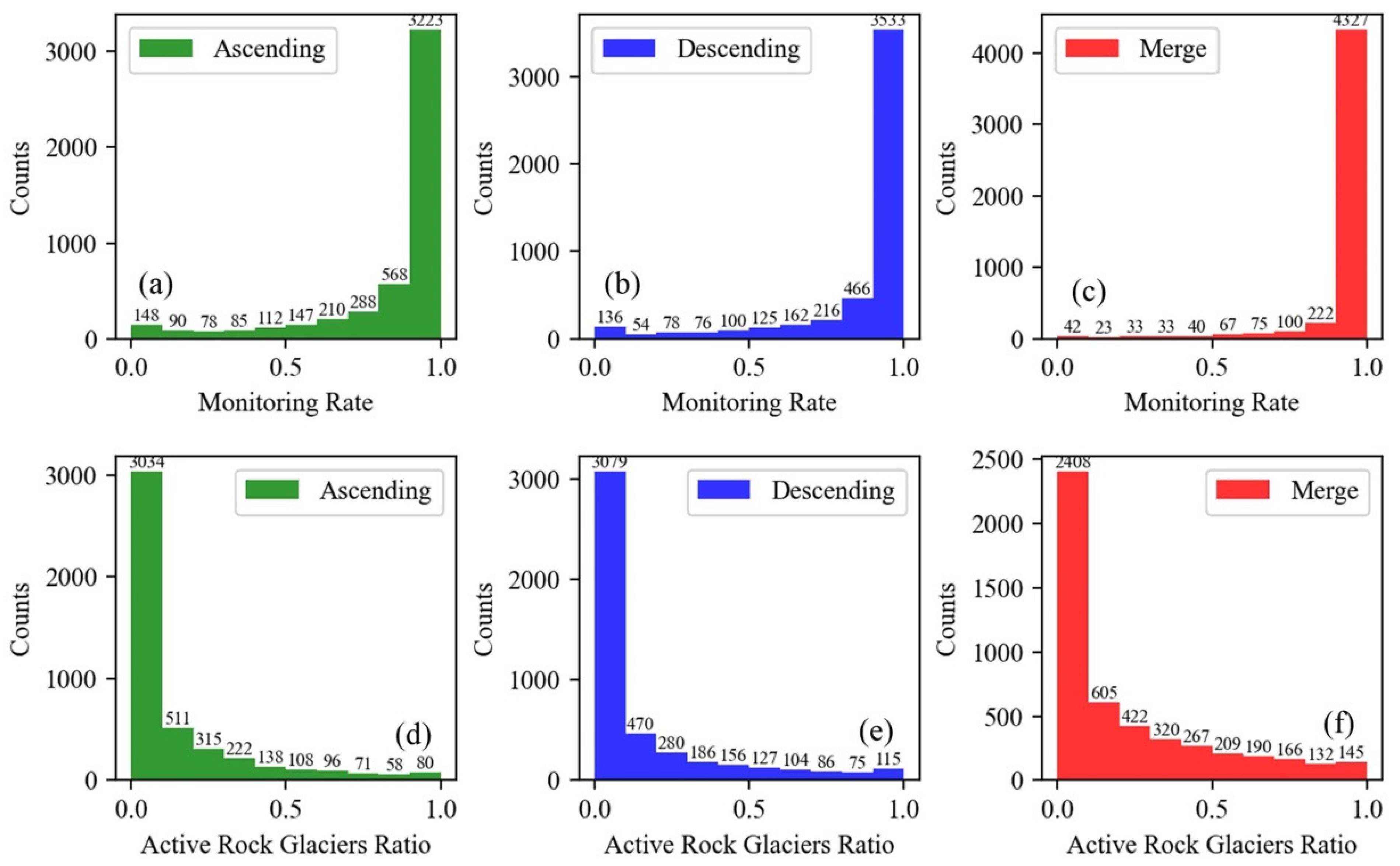
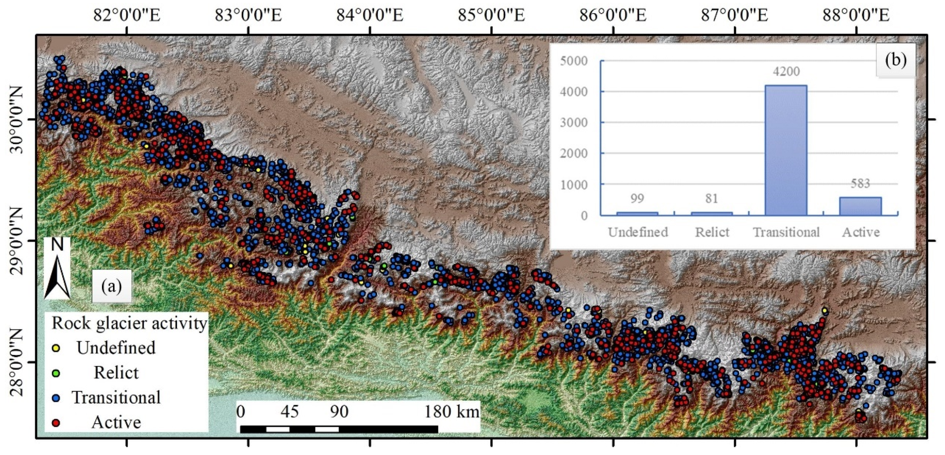
Based on regional MT-InSAR deformation estimates, the active thresholds of rock glaciers were 28.84 mm/y in the ascending orbit and 29.47 mm/y in the descending orbit. With these thresholds, about 32% of fine monitored rock glaciers had a ratio of active pixels greater than 10%. The percentage increased to 49% after merging the ascending and descending results. Following the criteria in the IPA Action Group guidelines of rock glacier activity classification, 12% of the recognized rock glaciers were active.

(3)

This work demonstrated the potential of the multi-baseline PS–DS network-based MT-InSAR for monitoring the activity of rock glaciers in an extensive periglacial environment. The use of a DTN network for the inversion of the deformation parameters provided a practical approach for suppressing the APS influence caused by the high reliefs in the periglacial zones of the Himalayas.

In future work, we will focus on investigating the seasonal deformation characteristics of rock glaciers and periglacial environment permafrost and on building and integrating a multivariate seasonal deformation model in the deformation estimation network.

References

- Berthling, I. Beyond Confusion: Rock Glaciers as Cryo-Conditioned Landforms. Geomorphology 2011, 131, 98–106. [Google Scholar] [CrossRef]
- Bonnaventure, P.P.; Lamoureux, S.F. The Active Layer: A Conceptual Review of Monitoring, Modelling Techniques and Changes in a Warming Climate. Prog. Phys. Geogr. 2013, 37, 352–376. [Google Scholar] [CrossRef]
- Jones, D.B.; Harrison, S.; Anderson, K.; Whalley, W.B. Rock Glaciers and Mountain Hydrology: A Review. Earth-Sci. Rev. 2019, 193, 66–90. [Google Scholar] [CrossRef]
- Liu, L.; Millar, C.I.; Westfall, R.D.; Zebker, H.A. Surface Motion of Active Rock Glaciers in the Sierra Nevada, California, USA: Inventory and a Case Study Using InSAR. Cryosphere 2013, 7, 1109–1119. [Google Scholar] [CrossRef] [Green Version]
- Jones, D.B.; Harrison, S.; Anderson, K.; Betts, R.A. Mountain Rock Glaciers Contain Globally Significant Water Stores. Sci. Rep. 2018, 8, 2834. [Google Scholar] [CrossRef] [Green Version]
- Liljedahl, A.K.; Boike, J.; Daanen, R.P.; Fedorov, A.N.; Frost, G.V.; Grosse, G.; Hinzman, L.D.; Iijma, Y.; Jorgenson, J.C.; Matveyeva, N.; et al. Pan-Arctic Ice-Wedge Degradation in Warming Permafrost and Its Influence on Tundra Hydrology. Nat. Geosci. 2016, 9, 312–318. [Google Scholar] [CrossRef]
- Bosson, J.B.; Lambiel, C. Internal Structure and Current Evolution of Very Small Debris-Covered Glacier Systems Located in Alpine Permafrost Environments. Front. Earth Sci. 2016, 4, 39. [Google Scholar] [CrossRef] [Green Version]
- Marcer, M.; Serrano, C.; Brenning, A.; Bodin, X.; Goetz, J.; Schoeneich, P. Evaluating the Destabilization Susceptibility of Active Rock Glaciers in the French Alps. Cryosphere 2019, 13, 141–155. [Google Scholar] [CrossRef] [Green Version]
- Biskaborn, B.K.; Smith, S.L.; Noetzli, J.; Matthes, H.; Vieira, G.; Streletskiy, D.A.; Schoeneich, P.; Romanovsky, V.E.; Lewkowicz, A.G.; Abramov, A.; et al. Permafrost Is Warming at a Global Scale. Nat. Commun. 2019, 10, 264. [Google Scholar] [CrossRef] [Green Version]
- Rouyet, L.; Lauknes, T.R.; Berthling, I. Recent Acceleration of a Rock Glacier Complex, Ádjet, Norway, Documented by 62 Years of Remote Sensing. Geophys. Res. Lett. 2018, 16, 8314–8323. [Google Scholar] [CrossRef] [Green Version]
- Boeckli, L.; Brenning, A.; Gruber, S.; Noetzli, J. A Statistical Approach to Modelling Permafrost Distribution in the European Alps or Similar Mountain Ranges. Cryosphere 2012, 6, 125–140. [Google Scholar] [CrossRef] [Green Version]
- Cao, B.; Li, X.; Feng, M.; Zheng, D. Quantifying Overestimated Permafrost Extent Driven by Rock Glacier Inventory. Geophys. Res. Lett. 2021, 48, e2021GL092476. [Google Scholar] [CrossRef]
- Kenner, R.; Pruessner, L.; Beutel, J.; Limpach, P.; Phillips, M. How Rock Glacier Hydrology, Deformation Velocities and Ground Temperatures Interact: Examples from the Swiss Alps. Permafr. Periglac. Process. 2020, 31, 3–14. [Google Scholar] [CrossRef]
- Ulrich, V.; Williams, J.G.; Zahs, V.; Anders, K.; Hfle, B. Measurement of Rock Glacier Surface Change over Different Timescales Using Terrestrial Laser Scanning Point Clouds. Earth Surf. Dyn. 2021, 9, 19–28. [Google Scholar] [CrossRef]
- Fey, C.; Krainer, K. Analyses of UAV and GNSS Based Flow Velocity Variations of the Rock Glacier Lazaun (Ötztal Alps, South Tyrol, Italy). Geomorphology 2020, 365, 107261. [Google Scholar] [CrossRef]
- Strozzi, T.; Delaloye, R.; Kääb, A.; Ambrosi, C.; Perruchoud, E. Combined Observations of Rock Mass Movements Using Satellite SAR Interferometry, Differential GPS, Airborne Digital Photogrammetry, and Airborne Photography Interpretation. J. Geophys. Res. Earth Surf. 2010, 115, F1. [Google Scholar] [CrossRef] [Green Version]
- Villarroel, C.D.; Beliveau, G.T.; Forte, A.P.; Monserrat, O.; Morvillo, M. DInSAR for a Regional Inventory of Active Rock Glaciers in the Dry Andes Mountains of Argentina and Chile with Sentinel-1 Data. Remote Sens. 2018, 10, 1588. [Google Scholar] [CrossRef] [Green Version]
- Kääb, A. Remote sensing of permafrost related problems and hazards. Permafr. Periglac. Process 2008, 19, 107–136. [Google Scholar] [CrossRef]
- Johnson, G.; Chang, H.; Fountain, A. Active rock glaciers of the contiguous United States: Geographic information system inventory and spatial distribution patterns. Earth Syst. Sci. Data. 2021, 13, 3979–3994. [Google Scholar] [CrossRef]
- Aoyama, M. Rock Glaciers in the Northern Japanese Alps: Palaeoenvironmental Implications since the Late Glacial. J. Quat. Sci. 2005, 20, 471–484. [Google Scholar] [CrossRef]
- Millar, C.I.; Westfall, R.D. Geographic, Hydrological, and Climatic Significance of Rock Glaciers in the Great Basin, USA. Arct. Antarct. Alp. Res. 2019, 51, 232–249. [Google Scholar] [CrossRef] [Green Version]
- Iasio, C.; Novali, F.; Corsini, A.; Mulas, M.; Branzanti, M.; Benedetti, E.; Giannico, C.; Tamburini, A.; Mair, V. COSMO SkyMed high frequency-high resolution monitoring of an alpine slow landslide, Corvara in Badia, Northern Italy. In Proceedings of the 2012 IEEE International Geoscience and Remote Sensing Symposium, Munich, Germany, 22–27 July 2012; pp. 7577–7580. [Google Scholar]
- Benoit, L.; Dehecq, A.; Pham, H.-T.; Vernier, F.; Trouvé, E.; Moreau, L.; Martin, O.; Thom, C.; Pierrot-Deseilligny, M.; Briole, P. Multi-Method Monitoring of Glacier d’Argentière Dynamics. Ann. Glaciol. 2015, 56, 118–128. [Google Scholar] [CrossRef] [Green Version]
- Kenyi, L.W.; Kaufmann, V. Estimation of Alpine Permafrost Surface Deformation Using InSAR Data. Int. Geosci. Remote Sens. Symp. 2001, 3, 1107–1109. [Google Scholar] [CrossRef]
- Nagler, T.; Mayer, C.; Rott, H. Feasibility of DINSAR for Mapping Complex Motion Fields of Alpine Ice- and Rock-Glaciers. In Proceedings of the Retrieval of Bio-and Geo-Physical Parameters from SAR Data for Land Applications, Sheffield, UK, 11–14 September 2001; Volume 475, pp. 377–382. [Google Scholar]
- Barboux, C.; Delaloye, R.; Lambiel, C. Inventorying Slope Movements in an Alpine Environment Using DInSAR. Earth Surf. Process. Landf. 2014, 39, 2087–2099. [Google Scholar] [CrossRef] [Green Version]
- Bhattacharya, A.; Mukherjee, K. Review on InSAR Based Displacement Monitoring of Indian Himalayas: Issues, Challenges and Possible Advanced Alternatives. Geocarto Int. 2017, 32, 298–321. [Google Scholar] [CrossRef]
- Rignot, E.; Hallet, B.; Fountain, A. Rock Glacier Surface Motion in Beacon Valley, Antarctica, from Synthetic-Aperture Radar Interferometry. Geophys. Res. Lett. 2002, 29, 48-1–48-4. [Google Scholar] [CrossRef] [Green Version]
- Eckerstorfer, M.; Eriksen, H.Ø.; Rouyet, L.; Christiansen, H.H.; Lauknes, T.R.; Blikra, L.H. Comparison of Geomorphological Field Mapping and 2D-InSAR Mapping of Periglacial Landscape Activity at Nordnesfjellet, Northern Norway. Earth Surf. Process. Landf. 2018, 43, 2147–2156. [Google Scholar] [CrossRef]
- Dini, B.; Manconi, A.; Loew, S. Investigation of Slope Instabilities in NW Bhutan as Derived from Systematic DInSAR Analyses. Eng. Geol. 2019, 259, 105111. [Google Scholar] [CrossRef]
- Wang, X.; Liu, L.; Zhao, L.; Wu, T.; Li, Z.; Liu, G. Mapping and Inventorying Active Rock Glaciers in the Northern Tien Shan of China Using Satellite SAR Interferometry. Cryosphere 2017, 11, 997–1014. [Google Scholar] [CrossRef] [Green Version]
- Barboux, C.; Strozzi, T.; Delaloye, R.; Wegmüller, U.; Collet, C. Mapping Slope Movements in Alpine Environments Using TerraSAR-X Interferometric Methods. ISPRS J. Photogramm. Remote Sens. 2015, 109, 178–192. [Google Scholar] [CrossRef] [Green Version]
- Strozzi, T.; Caduff, R.; Jones, N.; Barboux, C.; Delaloye, R.; Bodin, X.; Kääb, A.; Mätzler, E.; Schrott, L. Monitoring Rock Glacier Kinematics with Satellite Synthetic Aperture Radar. Remote Sens. 2020, 12, 559. [Google Scholar] [CrossRef] [Green Version]
- Necsoiu, M.; Onaca, A.; Wigginton, S.; Urdea, P. Rock Glacier Dynamics in Southern Carpathian Mountains from High-Resolution Optical and Multi-Temporal SAR Satellite Imagery. Remote Sens. Environ. 2016, 177, 21–36. [Google Scholar] [CrossRef] [Green Version]
- Ferretti, A.; Prati, C.; Rocca, F. Permanent Scatterers in SAR Interferometry. IEEE Trans. Geosci. Remote Sens. 2001, 39, 8–20. [Google Scholar] [CrossRef]
- Berardino, P.; Fornaro, G.; Lanari, R.; Sansosti, E. A New Algorithm for Surface Deformation Monitoring Based on Small Baseline Differential SAR Interferograms. IEEE Trans. Geosci. Remote Sens. 2002, 40, 2375–2383. [Google Scholar] [CrossRef] [Green Version]
- Du, W.; Ji, W.; Xu, L.; Wang, S. Deformation Time Series and Driving-Force Analysis of Glaciers in the Eastern Tienshan Mountains Using the Sbas Insar Method. Int. J. Environ. Res. Public Health 2020, 17, 2836. [Google Scholar] [CrossRef] [Green Version]
- Daout, S.; Sudhaus, H.; Kausch, T.; Steinberg, A.; Dini, B. Interseismic and Postseismic Shallow Creep of the North Qaidam Thrust Faults Detected with a Multitemporal InSAR Analysis. J. Geophys. Res. Solid Earth 2019, 124, 7259–7279. [Google Scholar] [CrossRef]
- Survey, F.G.; Foumelis, M.; Survey, F.G.; Raucoules, D.; Survey, F.G.; Michele, M.D.; Survey, F.G. Landslide Mapping and Monitoring Using Persistent Scatterer Interferometry (PSI) Technique in the French Alps. Remote Sens. 2020, 12, 1305. [Google Scholar] [CrossRef] [Green Version]
- Rouyet, L.; Lauknes, T.R.; Christiansen, H.H.; Strand, S.M.; Larsen, Y. Seasonal Dynamics of a Permafrost Landscape, Adventdalen, Svalbard, Investigated by InSAR. Remote Sens. Environ. 2019, 231, 111236. [Google Scholar] [CrossRef]
- Yhokha, A.; Chang, C.P.; Goswami, P.K.; Yen, J.Y.; Lee, S.I. Surface Deformation in the Himalaya and Adjoining Piedmont Zone of the Ganga Plain, Uttarakhand, India: Determined by Different Radar Interferometric Techniques. J. Asian Earth Sci. 2015, 106, 119–129. [Google Scholar] [CrossRef]
- Øverli, H.; Rune, T.; Larsen, Y.; Corner, G.D.; Bergh, S.G. Visualizing and Interpreting Surface Displacement Patterns on Unstable Slopes Using Multi-Geometry Satellite SAR Interferometry ( 2D InSAR ) Remote Sensing of Environment Visualizing and Interpreting Surface Displacement Patterns on Unstable Slopes Using. Remote Sens. Environ. 2017, 191, 297–312. [Google Scholar] [CrossRef] [Green Version]
- Dini, B.; Daout, S.; Manconi, A.; Loew, S. Classification of Slope Processes Based on Multitemporal DInSAR Analyses in the Himalaya of NW Bhutan. Remote Sens. Environ. 2019, 233, 111408. [Google Scholar] [CrossRef]
- Reinosch, E.; Gerke, M.; Riedel, B.; Schwalb, A.; Ye, Q.; Buckel, J. Rock Glacier Inventory of the Western Nyainqêntanglha Range, Tibetan Plateau, Supported by InSAR Time Series and Automated Classification. Permafr. Periglac. Process. 2021, 32, 657–672. [Google Scholar] [CrossRef]
- Reinosch, E.; Buckel, J.; Dong, J.; Gerke, M.; Baade, J.; Riedel, B. InSAR Time Series Analysis of Seasonal Surface Displacement Dynamics on the Tibetan Plateau. Cryosphere Discuss. 2019, 14, 1633–1650. [Google Scholar] [CrossRef]
- Longépé, N.; Allain, S.; Ferro-Famil, L.; Pottier, E.; Durand, Y. Snowpack Characterization in Mountainous Regions Using C-Band SAR Data and a Meteorological Model. IEEE Trans. Geosci. Remote Sens. 2009, 47, 406–418. [Google Scholar] [CrossRef]
- Tsai, Y.L.S.; Dietz, A.; Oppelt, N.; Kuenzer, C. Remote Sensing of Snow Cover Using Spaceborne SAR: A Review. Remote Sens. 2019, 11, 1456. [Google Scholar] [CrossRef] [Green Version]
- Wasowski, J.; Bovenga, F. Investigating Landslides and Unstable Slopes with Satellite Multi Temporal Interferometry: Current Issues and Future Perspectives. Eng. Geol. 2014, 174, 103–138. [Google Scholar] [CrossRef]
- Notti, D.; Herrera, G.; Bianchini, S.; Meisina, C.; García-Davalillo, J.C.; Zucca, F. A Methodology for Improving Landslide PSI Data Analysis. Int. J. Remote Sens. 2014, 35, 2186–2214. [Google Scholar] [CrossRef]
- Ferretti, A.; Fumagalli, A.; Novali, F.; Prati, C.; Rocca, F.; Rucci, A. A New Algorithm for Processing Interferometric Data-Stacks: SqueeSAR. IEEE Trans. Geosci. Remote Sens. 2011, 49, 3460–3470. [Google Scholar] [CrossRef]
- Philipp, M.; Dietz, A.; Buchelt, S.; Kuenzer, C. Trends in Satellite Earth Observation for Permafrost Related Analyses—A Review. Remote Sens. 2021, 13, 1217. [Google Scholar] [CrossRef]
- Daout, S.; Dini, B.; Haeberli, W.; Doin, M.P.; Parsons, B. Ice Loss in the Northeastern Tibetan Plateau Permafrost as Seen by 16 Yr of ESA SAR Missions. Earth Planet. Sci. Lett. 2020, 545, 116404. [Google Scholar] [CrossRef]
- Jolivet, R.; Grandin, R.; Lasserre, C.; Doin, M.P.; Peltzer, G. Systematic InSAR Atmospheric Phase Delay Corrections from Global Meteorological Reanalysis Data Systematic InSAR Tropospheric Phase Delay Corrections from Global Meteorological Reanalysis Data. Geophys. Res. Lett. 2011, 38. [Google Scholar] [CrossRef] [Green Version]
- Bekaert, D.; Hooper, A.; Wright, T. A Spatially Variable Power Law Tropospheric Correction Technique for InSAR Data. J. Geophys. Res. Solid Earth 2015, 120, 1345–1356. [Google Scholar] [CrossRef]
- Kang, Y.; Lu, Z.; Zhao, C.; Xu, Y.; Kim, J.; Gallegos, A.J. InSAR Monitoring of Creeping Landslides in Mountainous Regions: A Case Study in Eldorado National Forest, California. Remote Sens. Environ. 2021, 258, 112400. [Google Scholar] [CrossRef]
- Jones, D.B.; Harrison, S.; Anderson, K.; Selley, H.L.; Wood, J.L.; Betts, R.A. The Distribution and Hydrological Significance of Rock Glaciers in the Nepalese Himalaya. Glob. Planet. Chang. 2018, 160, 123–142. [Google Scholar] [CrossRef] [Green Version]
- Owens, R.G.; Hewson, T. ECMWF Forecast User Guide. 2018. Available online: https://www.ecmwf.int/en/elibrary/16559-ecmwf-forecast-user-guide (accessed on 19 November 2021). [CrossRef]
- Jones, D.B.; Harrison, S.; Anderson, K.; Shannon, S.; Betts, R.A. Rock Glaciers Represent Hidden Water Stores in the Himalaya. Sci. Total Environ. 2021, 793, 145368. [Google Scholar] [CrossRef]
- RGIK. IPA Action Group Rock Glacier Inventories and Kinematics: Baseline Concepts Version 4.1. 2020. Available online: https://bigweb.unifr.ch/Science/Geosciences/Geomorphology/Pub/Website/IPA/Guidelines/V4/210801_Baseline_Concepts_Inventorying_Rock_Glaciers_V4.2.1.pdf (accessed on 19 November 2021).
- Qin, Y. Sentinel-1 Wide Swath Interferometry: Processing Techniques and Applications. Ph.D. Thesis, Purdue University Graduate School, West Lafayette, IN, USA, 2018; p. 132. [Google Scholar] [CrossRef]
- Wang, C.; Tang, Y.; Zhang, H.; You, H.; Zhang, W.; Duan, W.; Wang, J.; Dong, L.; Zhang, B. First Mapping of China Surface Movement Using Supercomputing Interferometric SAR Technique. Sci. Bull. 2021, 66, 1608–1610. [Google Scholar] [CrossRef]
- Wang, C.; Zhang, Z.; Zhang, H.; Zhang, B.; Tang, Y.; Wu, Q. Active Layer Thickness Retrieval of Qinghai-Tibet Permafrost Using the TerraSAR-X InSAR Technique. IEEE J. Sel. Top. Appl. Earth Obs. Remote Sens. 2018, 11, 4403–4413. [Google Scholar] [CrossRef]
- Wu, H.; Zhang, Y.; Kang, Y.; Lu, Z.; Cheng, X. Semi-Automatic Selection of Optimum Image Pairs Based on the Interferometric Coherence for Time Series SAR Interferometry. Remote Sens. Lett. 2019, 10, 1105–1112. [Google Scholar] [CrossRef]
- Jarvis, A.; Reuter, H.; Nelson, A.; Guevara, E. Hole-Filled SRTM for the Globe Version 3, from the CGIAR-CSI SRTM 90 m Database. 2008. Available online: https://srtm.csi.cgiar.org/srtmdata/ (accessed on 19 November 2021).
- Zhang, Z.; Wang, C.; Tang, Y.; Fu, Q.; Zhang, H. Subsidence Monitoring in Coal Area Using Time-Series InSAR Combining Persistent Scatterers and Distributed Scatterers. Int. J. Appl. Earth Obs. Geoinf. 2015, 39, 49–55. [Google Scholar] [CrossRef]
- Ma, P.; Lin, H. Robust Detection of Single and Double Persistent Scatterers in Urban Built Environments. IEEE Trans. Geosci. Remote Sens. 2016, 54, 2124–2139. [Google Scholar] [CrossRef]
- Ma, P.; Wang, W.; Zhang, B.; Wang, J.; Shi, G.; Huang, G.; Chen, F.; Jiang, L.; Lin, H. Remotely Sensing Large- and Small-Scale Ground Subsidence: A Case Study of the Guangdong–Hong Kong–Macao Greater Bay Area of China. Remote Sens. Environ. 2019, 232, 111282. [Google Scholar] [CrossRef]
- Wang, Y.; Zhu, X.X.; Bamler, R. Retrieval of Phase History Parameters from Distributed Scatterers in Urban Areas Using Very High Resolution SAR Data. ISPRS J. Photogramm. Remote Sens. 2012, 73, 89–99. [Google Scholar] [CrossRef] [Green Version]
- Zhang, B.; Wang, R.; Deng, Y.; Ma, P.; Lin, H.; Wang, J. Mapping the Yellow River Delta Land Subsidence with Multitemporal SAR Interferometry by Exploiting Both Persistent and Distributed Scatterers. ISPRS J. Photogramm. Remote Sens. 2019, 148, 157–173. [Google Scholar] [CrossRef]
- Tang, Y.; Zhang, Z.; Wang, C.; Zhang, H.; Wu, F.; Zhang, B.; Liu, M. The Deformation Analysis of Wenjiagou Giant Landslide by the Distributed Scatterer Interferometry Technique. Landslides 2018, 15, 347–357. [Google Scholar] [CrossRef]
- Zhang, X.; Zhang, H.; Wang, C.; Tang, Y.; Zhang, B.; Wu, F. Soil Moisture Estimation Based on the Distributed Scatterers Adaptive Filter over the QTP Permafrost Region Using Sentinel-1 and High-Resolution TerraSAR-X Data. Int. J. Remote Sens. 2020, 42, 902–928. [Google Scholar] [CrossRef]
- Zhang, Z.; Wang, C.; Wang, M.; Wang, Z.; Zhang, H. Surface Deformation Monitoring in Zhengzhou City from 2014 to 2016 Using Time-Series InSAR. Remote Sens. 2018, 10, 1731. [Google Scholar] [CrossRef] [Green Version]
- Zhang, X.; Zhang, H.; Wang, C.; Tang, Y.; Zhang, B.; Wu, F.; Wang, J.; Zhang, Z. Time-Series InSAR Monitoring of Permafrost Freeze-Thaw Seasonal Displacement over Qinghai-Tibetan Plateau Using Sentinel-1 Data. Remote Sens. 2019, 11, 1000. [Google Scholar] [CrossRef] [Green Version]
- Zhu, X.; Dong, Z.; Yu, A.; Wu, M.; Li, D.; Zhang, Y. New Approaches for Robust and Efficient Detection of Persistent Scatterers in SAR Tomography. Remote Sens. 2019, 11, 356. [Google Scholar] [CrossRef] [Green Version]
- Hansen, P.C.; O’Leary, D.P. The Use of the L-Curve in the Regularization of Discrete Ill-Posed Problems. SIAM J. Sci. Comput. 1993, 14, 1487–1503. [Google Scholar] [CrossRef]
- Cultrera, A.; Callegaro, L. A Simple Algorithm to Find the L-Curve Corner in the Regularisation of Ill-Posed Inverse Problems. IOP SciNotes 2020, 1, 025004. [Google Scholar] [CrossRef]
- Navarro, J.A.; Tomás, R.; Barra, A.; Pagán, J.I.; Reyes-Carmona, C.; Solari, L.; Vinielles, J.L.; Falco, S.; Crosetto, M. ADAtools: Automatic Detection and Classification of Active Deformation Areas from PSI Displacement Maps. ISPRS Int. J. Geo-Inf. 2020, 9, 584. [Google Scholar] [CrossRef]
- Barra, A.; Solari, L.; Béjar-Pizarro, M.; Monserrat, O.; Bianchini, S.; Herrera, G.; Crosetto, M.; Sarro, R.; González-Alonso, E.; Mateos, R.M.; et al. A Methodology to Detect and Update Active Deformation Areas Based on Sentinel-1 SAR Images. Remote Sens. 2017, 9, 1002. [Google Scholar] [CrossRef] [Green Version]
- RGIK. Rock Glacier Kinematics as an Associated Parameter of ECV Permafrost (Version 3.0). 2021. Available online: https://bigweb.unifr.ch/Science/Geosciences/Geomorphology/Pub/Website/IPA/RGK/20211102_RockGlacierKinematics_V3.pdf (accessed on 19 November 2021).
- Yunjun, Z.; Fattahi, H.; Amelung, F. Small Baseline InSAR Time Series Analysis: Unwrapping Error Correction and Noise Reduction. Comput. Geosci. 2019, 133, 104331. [Google Scholar] [CrossRef] [Green Version]
- Zhou, C.; Gong, H.; Chen, B.; Gao, M.; Cao, Q.; Cao, J.; Duan, L.; Zuo, J.; Shi, M. Land Subsidence Response to Different Land Use Types and Water Resource Utilization in Beijing-Tianjin-Hebei, China. Remote Sens. 2020, 12, 457. [Google Scholar] [CrossRef] [Green Version]
- López-Quiroz, P.; Doin, M.-P.; Tupin, F.; Briole, P.; Nicolas, J.-M. Time Series Analysis of Mexico City Subsidence Constrained by Radar Interferometry. J. Appl. Geophys. 2009, 69, 1–15. [Google Scholar] [CrossRef]
- Doin, M.-P.; Lasserre, C.; Peltzer, G.; Cavalié, O.; Doubre, C. Corrections of Stratified Tropospheric Delays in SAR Interferometry: Validation with Global Atmospheric Models. J. Appl. Geophys. 2009, 69, 35–50. [Google Scholar] [CrossRef]
- Bekaert, D.P.S. Spaceborne Synthetic Aperture Radar Survey of Subsidence in Hampton Roads, Virginia (USA). Sci. Rep. 2017, 7, 14752. [Google Scholar] [CrossRef] [PubMed] [Green Version]
- Brencher, G.; Handwerger, A.L.; Munroe, J.S. InSAR-Based Characterization of Rock Glacier Movement in the Uinta Mountains, Utah, USA. Cryosphere 2021, 15, 4823–4844. [Google Scholar] [CrossRef]
- Kääb, A.; Strozzi, T.; Bolch, T.; Caduff, R.; Trefall, H.; Stoffel, M.; Kokarev, A. Inventory, Motion and Acceleration of Rock Glaciers in Ile Alatau and Kungöy Ala-Too, Northern Tien Shan, since the 1950s. Cryosphere Discuss. 2020, 2020, 1–37. [Google Scholar] [CrossRef]
- Crosetto, M.; Monserrat, O.; Cuevas-González, M.; Devanthéry, N.; Crippa, B. Persistent Scatterer Interferometry: A Review. ISPRS J. Photogramm. Remote Sens. 2016, 115, 78–89. [Google Scholar] [CrossRef] [Green Version]
- Wang, B.; Zhao, C.; Zhang, Q.; Chen, L.; Chen, H. Update Two-Dimensional SAR Offset Tracking Deformation Time Series with Complex Sequential Least Squares Estimation. Remote Sens. Lett. 2021, 12, 247–256. [Google Scholar] [CrossRef]