Article

Sentinel-2 and Landsat-8 Observations for Harmful Algae Blooms in a Small Eutrophic Lake

1
Jiangsu Provincial Key Laboratory of Environmental Engineering, Jiangsu Provincial Academy of Environmental Science, Nanjing 210036, China
2
Key Laboratory of Watershed Geographic Sciences, Nanjing Institute of Geography and Limnology, Chinese Academy of Sciences, Nanjing 210008, China
*
Author to whom correspondence should be addressed.
Remote Sens. 2021, 13(21), 4479; https://doi.org/10.3390/rs13214479
Submission received: 18 October 2021 / Revised: 3 November 2021 / Accepted: 5 November 2021 / Published: 8 November 2021

Abstract

:
Widespread harmful cyanobacterial bloom is one of the most pressing concerns in lakes and reservoirs, resulting in a lot of negative ecological consequences and threatening public health. Ocean color instruments with low spatial resolution have been used to monitor cyanobacterial bloom in large lakes; however, they cannot be applied to small water bodies well. Here, the Multi-Spectral Instrument (MSI) onboard Sentinel-2A and -2B and the Operational Landsat Imager (OLI) onboard Landsat-8 were employed to assemble the virtual constellation and to track spatial and seasonal variations in floating algae blooms from 2016 to 2020 in a small eutrophic plateau lake: Lake Xingyun in China. The floating algae index (FAI) was calculated using Rayleigh-corrected reflectance in the red, near-infrared, and short-wave infrared bands. The MSI-derived FAI had a similar pattern to the OLI-derived FAI, with a mean absolute percentage error of 19.98% and unbiased percentage difference of 17.05%. Then, an FAI threshold, 0.0693, was determined using bimodal histograms of FAI images for floating algae extraction. The floating algae had a higher occurrence in the northern region than the southern region in this lake, whilst the occurrence of floating algae in summer and autumn was higher than that in spring and winter. Such a spatial and seasonal pattern was related to the variability in air temperature, wind speed and direction, and nutrients. The climatological annual mean occurrence of floating algae from 2016 to 2020 in Lake Xingyun exhibited a significant decrease, which was related to decreases in nutrients, resulting from efficient ecological restoration by the local government. This research highlighted the application of OLI-MSI virtual constellation on monitoring floating algae in a small lake, providing a practical and theoretical reference to monitor aquatic environments in small water bodies.

1. Introduction

With the dual effects of climate warming and intensified human activities, lake eutrophication and cyanobacterial bloom are extending across the globe [1,2,3,4], in particular in some shallow lakes, such as Lake Taihu (China), Lake Erie (U.S.), Lake Peipsi (Estonia), and Lake Bogoria (Kenya). Widespread cyanobacterial blooms pose an urgent demand to manage, mitigate, and restore perspectives in these inland water ecosystems. The aggregation of cyanobacteria in the surface water forms cyanobacterial scums, reducing the penetration of light radiation into the water column and impacting the growth of other phytoplankton, zooplankton, and fishes, significantly weakening the ecological functions of inland lakes [4,5]. Moreover, cyanobacteria could release Microcystin, which could threaten the safety of the drinking water and the health of animals on land and of human beings [6]. The Microcystin concentration in waters has been a critical indicator for evaluating the quality of drinking water by the World Health Organization (WHO), the Environmental Protection Agency (EPA) in the United States, and the EU Water Framework Directive [7]. Consequently, the monitoring of spatial and temporal variability in harmful algae blooms is critical to maintaining regional economic development and to safeguarding human health.
Satellite remote sensing has the capability of monitoring lake environments fast, such as floating algae blooms and water quality [8]. Over past years, a lot of studies employed ocean color instruments, such as the Moderate resolution Imaging Spectroradiometer (MODIS) (2000–present), Medium Resolution Imaging Spectrometer (MERIS, 2003–2012), and Ocean Land Colour Instrument (OLCI, 2016~) to monitor algae blooms in some large lakes around the world [9,10,11,12], owing to the fine spectral resolution and frequent revisit time (~1 day). However, the areas of many lakes were small; for example, 63.48% of global lakes are less than 100 km2 in size [13] (Figure 1a). The coarse spatial resolution of ocean color instruments (~300 m) does not obtain subtle details in small-sized lakes [14,15], which largely restricts the applications of remote sensing in aquatic environments [16].
Previous studies have monitored algal blooms using Landsat TM and ETM+ images [8,17,18]. However, lakes change quickly, particularly floating algae had different variations day to day [19,20]. As such, Landsat with a semi-monthly revisit time is insufficient to track spatiotemporal variations in algae blooms in the lakes [19]. Recently, several high-quality instruments with higher spatial resolutions than ocean color sensors, including the Sentinel-2 MSI (Multiple Spectral Instrument, 2A: 2015~; 2B: 2017~) and Landsat-8 OLI (Operational Land Imager, 2013~), were launched. These moderate-high spatial resolution instruments (10–60m) provide an opportunity to monitor small-sized lakes and to understand the variability in algae blooms profoundly [21,22,23]. Furthermore, Pahlevan et al. [24] demonstrates that the radiometric performance between Sentinel-2 MSI and Landsat-8 OLI is consistent and that they could provide comparable observations in inland lakes. The harmonized images of MSI and OLI have also been used to monitor phytoplankton bloom [25], lake water clarity [26], chlorophyll-a, and turbidity in the rivers [27].
This research aims to use MSI and OLI to generate a time series of cyanobacterial blooms (where they form floating scums) in a small eutrophic lake to support the analysis on how and why the floating algae varies. Specifically, we aim (1) to evaluate the agreement of Rayleigh-corrected reflectance between MSI and OLI; (2) to adapt an algorithm to detect floating algae from OLI and MSI imagery based on the floating-algae-index (FAI); and (3) to generate the spatial and seasonal variations in floating algae from 2016 to 2020 and, subsequently, to relate the variability to the meteorology and nutrients. This research is anticipated to extend the application of the high spatial resolution image on monitoring lakes and to improve the spatial details of aquatic remote sensing.

2. Materials and Methods

2.1. Study Area

Lake Xingyun (24°17′–24°23′ N, 102°45′–102°48′ E) is a eutrophic freshwater lake with an elevation of approximately 1722 m in Yunnan province located in the Yunan-Guizhou Plateau of China. It has a surface area of 34.71 km2 and an average water depth of 5.3 m (Figure 1) with a 10.5 km length and 5.8 km width. Lake Xingyun is in the subtropical monsoon climate with an 848.7 mm precipitation and averaged air temperature of 15.9 °C. The summer and autumn are cloudy and rainy, particularly for the period from June to October. Due to economic development, Lake Xingyun has been eutrophic since 1993 and frequent floating algae blooms recently occurred, raising a concern to monitor the spatial and temporal variation in floating algae. The common ocean color instruments had coarse spatial resolutions (~300 m) so those small lakes could not be observed sufficiently. For example, OLCI and VIIRS imagery in Lake Xingyun does not show the spatial details of lakes. In contrast, Sentinel-2B MSI image exhibited evident floating algae scums over waters (Figure 1).

2.2. Satellite Data Processing

Landsat-8 (LC08) OLI (2013~present), Sentinel-2A (S2A) MSI (2015~present), and Sentinel-2B (S2B) MSI (2017~present) were employed to extract the floating algae in Lake Xingyun. The online browse images were first examined visually, and a total of 152 scenes MSI and OLI Level-1 imagery with minimal cloud cover from 2016 to 2020 were obtained from the European Space Agency (ESA) (https://scihub.copernicus.eu, accessed on 16 September 2021) and the United States Geological Survey (USGS) (https://earthexplorer.usgs.gov, accessed on 16 September 2021), respectively. The annual and monthly available number of images of minimal cloud-cover are presented in Table 1. Due to the relatively long revisit frequency of MSI and OLI virtual constellation, (e.g., ~ 6 days for S2A+ LC08 and ~3.8 days for S2A+S2B+ LC08 in [28]), OLI or MSI images with minimal cloud did not include several months in 2016–2018 owing to frequent cloudy and rainy days. These data are well georeferenced and calibrated radiance data at visible and infrared bands, with the wavelengths at 443, 482, 561, 655, 865, 1609, and 2201 nm for OLI and 444, 497, 560, 665, 704, 740, 783, 843, 865, 1613, and 2200 nm for MSI [29]. There was a slight difference in wavelength and spectral response functions between Sentinel-2A and 2B MSI, but their band-averaged radiance or reflectance had minor differences [30], so that they were usually regarded as the same in previous studies [31,32]. We removed the absorption of water vapor, ozone, and Rayleigh scattering to obtain Rayleigh-corrected reflectance (Rrc, dimensionless) using Equation (1) [33,34].
R r c = π L t , λ F 0 , λ c o s θ 0 R r , λ
where λ is the wavelength (nm), Lt is the at-sensor radiance, Rr is the Rayleigh reflectance, F0 is extraterrestrial solar irradiance, θ0 is the solar zenith angle.
Specifically, OLI and MSI Rrc data were estimated using the latest ACOLITE software package (https://github.com/acolite, accessed on 16 September 2021). The gains were set to unity. In the processing, ancillary data (e.g., meteorology and ozone) and a digital elevation model (DEM) were used. The MSI data with 10 m, 20 m, and 60 m resolutions were mapped at the spatial resolution of 10 m for the floating algae extraction, while the OLI data were at 30 m.
To eliminate the influence of the land adjacency effects (LAEs), we used a statistical method to exclude those pixels with potential impacts of LAEs [35]. The ratio between Rrc for examined pixel and referenced pixels (assumed to be not affected by LAEs) along the transect from land to water tended to be approximately 1 when the pixel was away from five pixels to the land, suggesting that LAEs could be neglected (at least minimized) after excluding five pixels near the land.

2.3. Floating Algae Extraction

2.3.1. Floating Algae Index (FAI)

The significant peak at the near-infrared band of reflectance caused by the floating algae is the theoretical principle to distinguish it from water pixels using optical satellite image data. For example, MSI-derived Rrc image captured an obvious algae scums on 12 November 2020, and Rrc at the near-infrared (i.e., Rrc(NIR)) in the pixel covered by floating algae was significantly higher than that in the normal waters. Rrc(NIR) in the thick scums (Pin 3 in Figure 2c) was also higher than that in thin scums (e.g., Pin 3 in Figure 2c). The FAI proposed by [9] was selected to extract floating algae in Lake Xingyun from MSI and OLI image data. MSI and OLI do not equip the band near ~1240 nm; thus, we adapted the original FAI using the band of ~1600 nm.
F A I = R r c , N I R R r c , N I R
R r c , N I R = R r c , r e d + ( R r c , S W I R R r c , R e d ) × λ N I R λ R e d λ S W I R λ R e d
where Rrc,Red, Rrc,NIR, and Rrc,SWIR are Rayleigh-corrected reflectance of the red band (~660 nm), NIR band (~865 nm), and short-wave infrared (SWIR) band (~1600 nm) of MSI and OLI, respectively.

2.3.2. Land and Cloud Masking

The pixels of land and cloud with high FAI values mat be incorrectly recognized as floating algae. The water boundary was extracted using a scheme of normalized difference water index (NDWI) segmentation, ensuring that each image had an accurate water boundary. Some studies used the FMask method to recognize clouds over the lakes [3], but this approach did not include samples of floating algae [36], suggesting that FMask could not distinguish floating algae and cloud pixels well [19]. The ocean color community usually used the threshold of Rrc at the NIR and SWIR bands, such as 0.018 at 2130 nm for MODIS image [37], to remove clouds, yet these thresholds may remove pixels covered by floating areas as well. In this study, we interactively outlined the clouds using ENVI software to remove cloud pixels manually.

2.3.3. FAI Threshold to Distinguish Floating Algae

The determination of the FAI threshold to distinguish floating algae and water pixels is the most crucial task. Previous studies used FAI gradient images to determine threshold [38]. The several attempts found that the maximum of FAI gradient imagery was easily influenced by intensity of floating algae in Lake Xingyun. In fact, the FAI image with floating algae always presented a bimodal histogram (Figure 2d), where the left histogram with low FAI was water and the right peak with high FAI corresponded to floating algae area. Thus, we employed a histogram of the FAI image to determine this critical value.
For each FAI image after masking clouds and lands, the histogram of FAI was generated. The FAI image with unimodal histogram was not used to determine the FAI threshold due to the failed assumption with this approach. For the bimodal histogram or multimodal histogram, the threshold of FAI was determined using Equation (4), as illustrated in Figure 2d.
T = μ w × σ F A + μ F A × σ w μ w + μ F A
where μw and μFA are the mean values of water peak and floating algae peak, respectively, and σw and σFA are the corresponding standard deviations. They are the parameters of each Gaussian distribution and could be calculated in the fittings of functions.
The method was applied on each image to determine the FAI threshold to extract floating algae, and it obtained satisfactory performance. However, in some images where algae scums are small, this method failed due to fewer algae pixels forming a nearly unimodal histogram. After several examinations, the final FAI threshold, about 0.0693, was determined using the mean minus standard deviation of all FAI thresholds of images. We did not use the value that means − 2 × standard deviation by Hu et al., (2010) [38] due to the short study period and insufficient satellite images. This value was finally chosen as a time-independent FAI threshold to extract floating algae.

2.4. Evaluation of Agreement between MSI and OLI Data

Although MSI and OLI had comparable performances in monitoring waters [24], they still have different spectral settings, including center wavelength bandwidth and signal-to-noise ratio (Figure 3). Here, the agreement of MSI- and OLI-derived Rrc were evaluated based on the same-day images. We choose three scenes same-day MSI and OLI with minimal clouds from 2016 to 2020, including an image with floating algae. The averaged time difference between OLI and MSI data was about 5.6 min, suggesting nearly the same water environment as Lake Xingyun in the evaluation. These images were processed to generate Rrc data in ACOLITE. Then, these three MSI Rrc data were resampled to 30 m (i.e., the resolution of OLI) using a sharpening scheme in SeaDAS software [39]. After removal of the clouds and lands, about 300,000 OLI-MSI matchups were obtained to evaluate the consistency of Rrc and FAI. Detailed results can be found in Section 3.1.

2.5. Meteorological Data

Daily air temperature (°C), wind speed (m s−1), and precipitation (mm) in Yuxi meteorological station near Lake Xingyun were download from the National Meteorological Information Center, China (http://data.cma.cn, accessed on 16 September 2021) from 2016 to 2020. Monthly data were calculated to analyze the relations with temporal variations in floating algae.

2.6. Performance Metrics

Several statistical metrics were used to compare the differences between satellite derived products, such as Rrc data and FAI value. These metrics included the coefficient of determination (R2), the mean absolute percentage difference (MAPD), and the unbiased percentage difference (UPD). Their equations were defined as follows:
M A P D =   1 N i = 1 N | X i Y i | X i × 100 %
U P D ( % ) =   1 N i = 1 N | X i Y i | X i + Y i × 200 %
where N is the number of data pairs, and Xi and Yi denote the ith data pairs evaluated.

3. Results

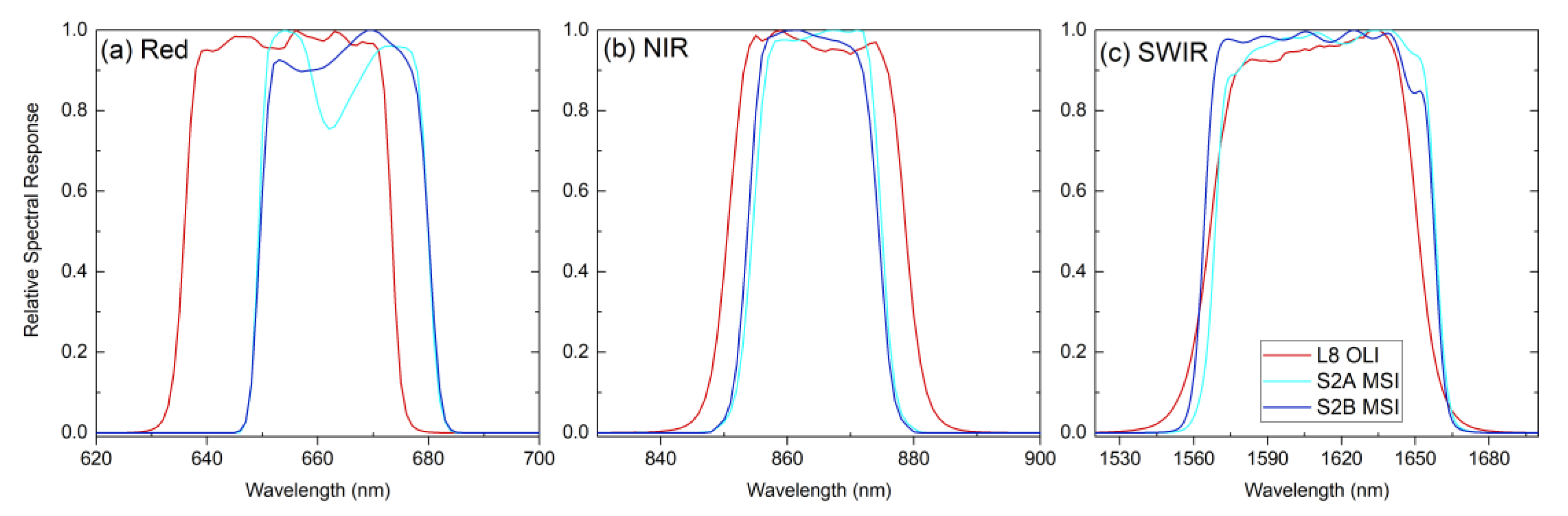
3.1. Agreement between OLI and MSI

Figure 4 shows a comparison of Rrc estimates and FAI values between MSI and OLI in Lake Xingyun. The consistency of Rrc between OLI and MSI was evaluated using 300,000 matchups. Overall, there are no obvious overestimations or underestimations for Rrc estimates among any of the three bands at ~665 nm, ~859 nm, and ~1610 nm, and the point-pairs are evenly distributed along both sides of the 1:1 line, while the slope was slightly higher than the unity. Specifically, Rrc measurements in the red band had better agreement than other bands (R2 = 0.85, MAPD = 12.68%, UPD = 12.66%) (Figure 4b), where most of the points (e.g., 0.03–0.1) were distributed evenly along with the unity. Although Rrc matchups at the band at ~865 nm and ~1610 nm were distributed along line 1:1, some of the points slightly deviated the unity line (Figure 4a,c), suggesting worse Rrc agreement in the NIR and SWIR bands than red band (865 nm: R2 = 0.78, MAPD = 11.91%, and UPD = 17.75%; 1610 nm: MAPD = 17.64% and UPD = 24.31%). The slight deviation for Rrc measurements between MSI and OLI in the NIR and SWIR bands could be related to the low SNRs.
The FAI of OLI and MSI was calculated by the three bands above exhibited good agreements, with an MAPD of 19.98% and an UPD of 17.05% (Figure 4d). Although some FAI matchups deviated from the unity line, these point pairs were low in scatter density. After removing matchups with a scatter density less than 10, the calibration coefficients between OLI and MSI were established: MSI‘(FAI) = 0.9416 × MSI(FAI) + 0.0019 (R2 = 0.88, p < 0.001). With this equation, MSI-derived FAI were converted to the same level of OLI (i.e., MSI‘(FAI)).

3.2. Performance of the Algorithm

Figure 5 presents examples of extracting floating algae in LC08 OLI, and S2A and S2B MSI images. The FAI images had similar patterns with the false-color composite image (FRGB), suggesting the validity of FAI on floating algae identification. The histograms of FAI showed obvious bimodal patterns, and the threshold to split those two peaks was located near 0.06. The extracted area of floating algae by FAI ≥ 0.0693 was consistent with the false-color composite image shown. Likewise, this approach did not recognize the clouds pixels as the floating algae because FAI was initially designed to reduce the thin clouds on the water.
Figure 6 illustrates the applications of the FAI threshold of 0.0693 on extracting floating algae in other lakes and reservoirs worldwide, such as Lake Dianchi (Yunnan, China), Nierji Reservoir (Heilongjiang, China), Lake Clear (California, CA, USA) and Lake Turawskie (Turawa, Poland). Obvious floating algae could be found in these lakes using FRGB images of Landsat-8 OLI and Sentinel-2 MSI. The floating algae extracted by FAI ≥ 0.0693 was consistent with the FRGB image basically; however, the results had deviations from that extracted by the unique FAI threshold of each lake. The specific value was determined using a bimodal histogram of FAI derived by each OLI or MSI Rrc data. The proposed threshold had 21.9% and 36.6% underestimations in Lake Dianchi and Lake Clear, respectively, while it overestimated 46.5% in Lake Turawskie. The difference in floating algae distribution possibly resulted from the different water constituents and phytoplankton types. A detailed discussion is provided in Section 4.1.

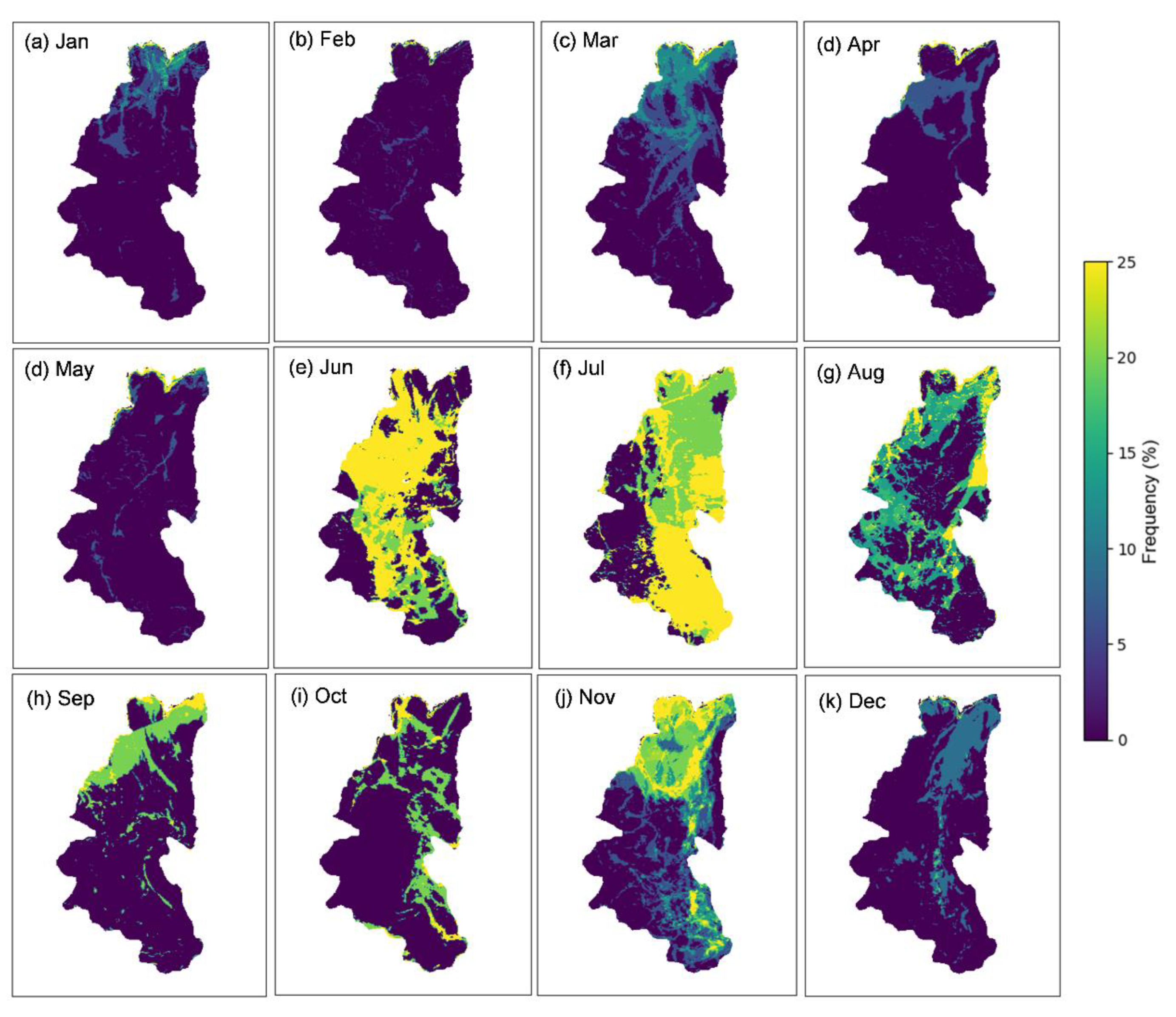
3.3. Spatial and Temporal Variations in Floating Algae

The distribution of floating algae derived by each MSI or OLI image was used to generated the climatological annual and monthly mean occurrences of floating algae in Lake Xinyun from 2016 to 2020. The occurrence of floating algae for each pixel is the ratio between the number of floating algae observations and total valid observations. Whilst the maximum area of floating algae in each month was obtained. This spatial and seasonal variability in floating algae was related to the variations in air temperature, wind speed, wind direction, and precipitation subsequently.
Figure 7 mapped the spatial distribution of climatological mean floating algae occurrence from 2016 to 2020, where the last panel is the mean results for the entire studied period. All regions in Lake Xinyun had significant floating algae, and the occurrence of floating algae in the northern and eastern regions was higher than in other areas. The occurrence of floating algae was between 10% to 15% in the northern and east area. The annual mean occurrence of floating algae had different distributions in different regions. For example, floating algae was mainly distributed in the northern region in the period of 2016–2018, whereas it mainly occurred in the northwest area in 2019 and in the central region in 2020 (Figure 7 and Figure 8a). In general, the occurrence of floating algae exhibited a decreasing trend from 2016 to 2020, where the mean occurrence was reduced to 5% in 2020 from 20% in 2016. Additionally, the maximum area of floating algae had a similar decrease in Lake Xingyun (Figure 8a). It was greater than 10 km2 from 2016 to 2017 and was lower than 5 km2 in 2020. Although the images to extract floating algae areas in 2016 and 2017 lacked some images in summer due to the cloudy and rainy conditions, it still captured high floating algae occurrence.
Figure 9 presents the maps of climatological monthly mean floating algae occurrence from 2016 to 2020 in Lake Xingyun. The occurrence of floating algae was high from June to November, where the occurrence in June and July was highest (19.51% in June and 20.15% in July) and was lowest in February (0.005%). It should be noted that relatively high floating algae occurrence (~15%) was reported in March in northern Lake Xingyun. The spatial distribution of floating algae was different in different seasons. The floating algae occurred in the entire lake in June and July, while the floating algae were mainly present in the northern region in November.

4. Discussion

4.1. Accuray and Applicability of the Algorithm

MSI and OLI had comparable radiometric performance to observe aquatic environments, and they are the candidates to build virtual constellations as well [24]. Although MSI and OLI had different spectral settings, including central wavelength and bandwidth (Figure 3), Rrc at the bands of red, NIR, and SWIR showed fair agreement (Figure 4), ensuring consistent FAI values between MSI and OLI. Furthermore, we calibrated the FAI of MSI to the same level of OLI, which can generate a consistent time series of floating algae with MSI and OLI virtual constellation. Although the distribution of floating algae scums extracted from MSI and OLI images were consistent with FRGB images (Figure 5 and Figure 6), the absolute accuracy with respect to the floating algae extractions were not further examined using the images with higher spatial resolution (e.g., ~1 m) because most of higher spatial resolution satellite images, such as Worldview-3 and Pléiades imagery [40], were commercial. In the future, the drone is anticipated to collect some aerial images when Landsat-8/9 and Sentinel-2A/2B overpass over the lake. The drone images could be used to manually delineate the subtle spatial distributions of floating algae, which would assist in validating and improving the results of floating algae extractions by satellite images.
The bimodal histogram of the FAI image was used to determine the FAI threshold by splitting the floating algae and water modes. This approach required accurate removal of clouds and lands; that is, FAI images only include floating algae and water pixels [38]. The land pixels could be removed using a threshold of NDWI [41]; however, it is still a challenge to exclude clouds over turbid waters. The state-of-the-art algorithms to remove clouds, such as FMask model, IdePIX approach, and the Rrc threshold in SWIR band, may recognize the pixels contaminated by floating algae as clouds [19,36,37] (Figure 10). Among these cloud masking methods in Figure 10, the Rrc threshold in SWIR band (Figure 10b) had fair performance in masking clouds and lands and was easy to use, even though it mistook some floating algae as clouds, meaning that the adaption of a threshold for a local lake may obtain fair results to feasibly exclude clouds for an operational application. In addition, a time series-based approach to analyze the frequency of cloud-like pixels was also used to mask cloud based on the idea that the lake is relatively stable and that clouds are dynamic. However, such methods did not perform as expected because the floating algae was also dynamic. As such, it was still a challenge to mask clouds for waters covered by floating algae scums.
In small lakes such as Lake Xingun, stray-light from the land or clouds could increase the high water albedo into satellite sensors, possibly influencing the extraction of floating algae. As such, LAEs could not be ignored for high spatial resolution images and small water bodies [42]. In general, operational satellite data processing in ocean color community employed a window to remove potential pixels influenced by LAEs. For example, SeaDAS software used a window of 7 × 5 to remove stray-light pixels, resulting in a data loss of more than 50% [43]. Following the method proposed by Feng and Hu [35], we removed five pixels near land to reduce LAEs. While efforts were made to remove adjacency effects, these are complex and difficult to avoid completely [44]. The spatial pattern of FAI near land in this study did not have apparent land adjacency effects, suggesting that the remaining impact of LAEs is minimal and does not significantly affect our study’s main conclusions.
Despite the FAI threshold used in Lake Xingyun (i.e., 0.0693) capturing thick floating scums in other lakes, it could not extract floating algae in other lakes (Figure 6), which had significantly different constituents and optical properties from that of Lake Xingyun. Such differences resulted in different Rrc spectra and FAI magnitudes [11]. In Lake Xingyun, the density of cyanobacteria accounted for 94.87–99.48% of phytoplankton, and Microcystis was dominant. However, algae and diatom are possibly the main phytoplankton in other water bodies. The different phytoplankton groups could cause various interactions with light as well [45]. Thus, it was almost difficult to extract floating algae in a broad region using one FAI threshold [46]. After adapting the FAI threshold based on water conditions, the proposed approach in this study was easy to extend to other areas.
The virtual constellation of MSI and OLI could improve, observing a frequency of 2.9 days [28], which meets the requirements for oceanologists and limnologists to study aquatic environments [24]. In Lake Xingyun, the MSI-OLI virtual constellation did not obtain enough cloud-free images from June to August due to the rainy and cloudy weather. In fact, MODIS with daily revisits only occasionally acquired cloud-free images in the area near Lake Xingyun in summer [47]. The cloud is still one of the challenges that hinder the optical satellite observation of the lake in the study region.

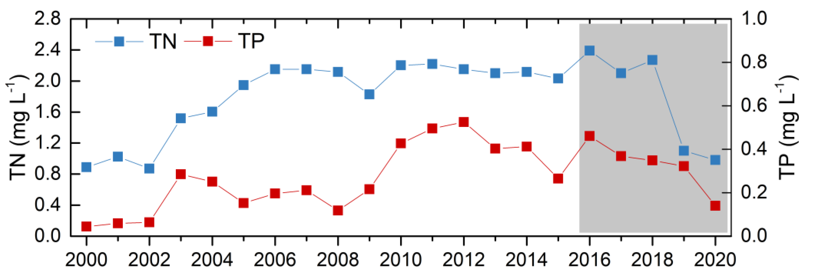
4.2. Driving Factors of Floating Algae in Lake Xingyun

Variability in algae blooms in lakes can be influenced by both climate and human activities. Warm water facilitates the growth of phytoplankton [48,49]. Winds can bring nutrients from the bottom layer to the surface by mixing, and precipitation can modulate variations in nutrients [50,51]. The presence of multiple factors complicates the understanding of the causes of floating algae blooms in lakes.
We found that the average occurrence of floating algae and the maximum area decreased since 2016 (Figure 7 and Figure 8a). Air temperature did not significantly decrease and wind did not have an increase (Figure 8b), suggesting that the meteorology was not the main factor in regulating the annual variation in floating algae in Lake Xingyun. The total nitrogen (TN) and total phosphorus (TP) in Lake Xingyun had significant decreases from 2016 to 2020 (Figure 11). TN reduced to 1.1 mg L−1 in 2020 from 2.4 mg L−1 in 2016, while TP decreased to 0.14 mg L−1 in 2020 from 0.46 mg L−1 in 2016. The decrease in nutrients in the lakes impedes the growth of cyanobacteria [52], so that floating algae is mitigated. Similar findings were reported in other lakes with cyanobacterial scums, such as Lake Taihu and Lake Chaohu [47,53,54]. In addition, the precipitation has been regarded as another factor that influences the occurrence of floating algae in Lake Dianchi, a neighbor eutrophic lake of Lake Xingyun [55], particularly on a long-term scale. The precipitation in Lake Xingyun had a decreasing trend from 2016 to 2020 (p < 0.05) (Figure 8d), reducing the loadings of the nutrients into lakes. The local environmental department carried out an ecological project termed “Sewage Interception and Restoration Project” in the southern region. This project was located between cropland and lake, largely mitigating agricultural pollution into the lake [56].
The cyanobacterial scums mainly broke out in summer and autumn (Figure 8a and Figure 9). Such seasonal variations primarily resulted from temperature, which was an important factor that impacts the growth of phytoplankton in waters [49]. The high temperature facilitated the growth of cyanobacteria in summer and autumn, resulting in a high occurrence of floating algae. Furthermore, the wind speed was low in summer and autumn (usually <2.0 m s−1) (Figure 8c). The cyanobacteria were easily aggregated in the surface water to form scums in weak mixing condition [57,58]. Similarly, Mu et al., (2019) showed that wind speeds less than 2.35 m s−1 in the dry season and 2.01 m s−1 in the rainy season would form cyanobacterial blooms in Lake Dianchi [55] and that wind speed had more effects on seasonal variability in cyanobacterial blooms. Additionally, Bi et al., (2019) also demonstrated that wind speed is a critical factor in regulating biomass in Lake Dianchi since wind speed is an important factor of hydrodynamics and water stability in waters [59].
The frequency of cyanobacterial blooms was higher in the northern region than in the center and south regions of Lake Xingyun (Figure 7 and Figure 9). The nutrient concentration in the north was higher than in the south in Lake Xingyun [60], which was consistent with the spatial pattern of floating algae. Additionally, the perennial southwest wind (Figure 8c) in Lake Xingyun drifts the cyanobacteria to the northern lake area. In Lake Taihu, the wind direction was also one of the reasons that cyanobacterial blooms were intensified in the northern and western lake regions [61].

5. Conclusions

This research employed Sentinel-2 MSI and Landsat-8 OLI images to monitor spatial and seasonal variability in floating algae in a small lake, Lake Xingyun, in the Yunan-Guizhou Plateau of China. The Rayleigh-corrected reflectance (Rrc) was used to calculate the floating algae index (FAI), which was subsequently used to recognize floating algae. The consistency of Rrc and FAI between MSI and OLI was evaluated to provide a same-level floating algae extraction from satellite imagery. A bimodal histogram was used to determine the FAI threshold to distinguish floating algae. The spatial and seasonal variability in floating algae in Lake Xingyun from 2016 to 2020 was performed. The meteorology and nutrients were related to the variations in floating algae in Lake Xingyun. The environmental project in 2015 significantly decreased the loadings of nutrients from the watershed into waters, resulting in decreases in floating algae occurrence in the lake. In the future, Sentinel-2A/B and Landsat-8/9 virtual constellations are anticipated to monitor small water bodies to aid in aquatic environmental management.

Author Contributions

Conceptualization, M.L.; methodology, M.L.; software, D.W.; formal analysis, M.L. and H.L.; data curation, Z.C. and X.S.; writing original draft preparation, M.L.; writing review and editing, all authors; supervision, H.L.; funding acquisition, M.L., Z.C. and H.L. All authors have read and agreed to the published version of the manuscript.

Funding

This research was funded by the National Natural Science Foundation of China (42101056 and 42101378), by the Provincial Natural Science Foundation of Jiangsu of China (BK20210989, BK20210953), by the Jiangsu Environmental Protection and Research Funds (2019003), and by the Taihu Lake Water Pollution Control Special Funds (TH2018402).

Data Availability Statement

The data presented in this study are available on reasonable request from the corresponding author.

Acknowledgments

We thank USGS and ESA for providing the Landsat and Sentinel-2 satellite data. Thanks to the two anonymous reviewers for their critical comments and suggestions.

Conflicts of Interest

The authors declare no conflict of interest.

References

  1. Wang, S.; Li, J.; Zhang, B.; Spyrakos, E.; Tyler, A.N.; Shen, Q.; Zhang, F.; Kuster, T.; Lehmann, M.K.; Wu, Y.; et al. Trophic state assessment of global inland waters using a MODIS-derived Forel-Ule index. Remote Sens. Environ. 2018, 217, 444–460. [Google Scholar] [CrossRef] [Green Version]
  2. Song, K.; Fang, C.; Jacinthe, P.A.; Wen, Z.; Liu, G.; Xu, X.; Shang, Y.; Lyu, L. Climatic versus Anthropogenic Controls of Decadal Trends (1983–2017) in Algal Blooms in Lakes and Reservoirs across China. Environ. Sci. Technol. 2021, 55, 2929–2938. [Google Scholar] [CrossRef] [PubMed]
  3. Ho, J.C.; Michalak, A.M.; Pahlevan, N. Widespread global increase in intense lake phytoplankton blooms since the 1980s. Nature 2019, 574, 667–670. [Google Scholar] [CrossRef] [PubMed]
  4. Huisman, J.; Codd, G.A.; Paerl, H.W.; Ibelings, B.W.; Verspagen, J.M.H.; Visser, P.M. Cyanobacterial blooms. Nat. Rev. Microbiol. 2018, 16, 471–483. [Google Scholar] [CrossRef] [PubMed]
  5. Guo, L. Ecology. Doing battle with the green monster of Taihu Lake. Science 2007, 317, 1166. [Google Scholar] [CrossRef] [PubMed]
  6. Chorus, I.; Bartram, J. Toxic Cyanobacteria in Water: A Guide to Their Public Health Consequences, Monitoring, and Management; Taylor & Francis: Abingdon, UK, 1999; Volume 18. [Google Scholar]
  7. Hayes, N.M.; Haig, H.A.; Simpson, G.L.; Leavitt, P.R. Effects of lake warming on the seasonal risk of toxic cyanobacteria exposure. Limnol. Oceanogr. Lett. 2020, 5, 393–402. [Google Scholar] [CrossRef]
  8. Duan, H.; Ma, R.; Xu, X.; Kong, F.; Zhang, S.; Kong, W.; Hao, J.; Shang, L. Two-Decade Reconstruction of Algal Blooms in China’s Lake Taihu. Environ. Sci. Technol. 2009, 43, 3522–3528. [Google Scholar] [CrossRef]
  9. Hu, C.M. A novel ocean color index to detect floating algae in the global oceans. Remote Sens. Environ. 2009, 113, 2118–2129. [Google Scholar] [CrossRef]
  10. Xing, Q.; Hu, C. Mapping macroalgal blooms in the Yellow Sea and East China Sea using HJ-1 and Landsat data: Application of a virtual baseline reflectance height technique. Remote Sens. Environ. 2016, 178, 113–126. [Google Scholar] [CrossRef]
  11. Qi, L.; Hu, C.; Mikelsons, K.; Wang, M.; Lance, V.; Sun, S.; Barnes, B.B.; Zhao, J.; Van der Zande, D. In search of floating algae and other organisms in global oceans and lakes. Remote Sens. Environ. 2020, 239, 111659. [Google Scholar] [CrossRef]
  12. Binding, C.E.; Greenberg, T.A.; Bukata, R.P. The MERIS Maximum Chlorophyll Index: Its merits and limitations for inland water algal bloom monitoring. J. Great Lakes Res. 2013, 39, 100–107. [Google Scholar] [CrossRef]
  13. Downing, J.A.; Prairie, Y.T.; Cole, J.J.; Duarte, C.M.; Tranvik, L.J.; Striegl, R.G.; McDowell, W.H.; Kortelainen, P.; Caraco, N.F.; Melack, J.M.; et al. The global abundance and size distribution of lakes, ponds, and impoundments. Limnol. Oceanogr. 2006, 51, 2388–2397. [Google Scholar] [CrossRef] [Green Version]
  14. Kutser, T. Quantitative detection of chlorophyll in cyanobacterial blooms by satellite remote sensing. Limnol. Oceanogr. 2004, 49, 2179–2189. [Google Scholar] [CrossRef]
  15. Olmanson, L.G.; Brezonik, P.L.; Bauer, M.E. Evaluation of medium to low resolution satellite imagery for regional lake water quality assessments. Water Resour. Res. 2011, 47, W09515. [Google Scholar] [CrossRef] [Green Version]
  16. Cao, Z.; Ma, R.; Duan, H.; Xue, K. Effects of broad bandwidth on the remote sensing of inland waters: Implications for high spatial resolution satellite data applications. ISPRS J. Photogramm. Remote Sens. 2019, 153, 110–122. [Google Scholar] [CrossRef]
  17. Zhao, D.; Li, J.; Hu, R.; Shen, Q.; Zhang, F. Landsat-satellite-based analysis of spatial–temporal dynamics and drivers of CyanoHABs in the plateau Lake Dianchi. Int. J. Remote Sens. 2018, 39, 8552–8571. [Google Scholar] [CrossRef]
  18. Ho, J.C.; Stumpf, R.P.; Bridgeman, T.B.; Michalak, A.M. Using Landsat to extend the historical record of lacustrine phytoplankton blooms: A Lake Erie case study. Remote Sens. Environ. 2017, 191, 273–285. [Google Scholar] [CrossRef]
  19. Feng, L.; Dai, Y.; Hou, X.; Xu, Y.; Liu, J.; Zheng, C. Concerns about phytoplankton bloom trends in global lakes. Nature 2021, 590, E35–E47. [Google Scholar] [CrossRef]
  20. Qi, L.; Hu, C.; Visser, P.M.; Ma, R. Diurnal changes of cyanobacteria blooms in Taihu Lake as derived from GOCI observations. Limnol. Oceanogr. 2018, 63, 1711–1726. [Google Scholar] [CrossRef] [Green Version]
  21. Ruddick, K.; Vanhellemont, Q.; Dogliotti, A.; Nechad, B.; Pringle, N.; Van der Zande, D. New opportunities and challenges for high resolution remote sensing of water colour. In Proceedings of the Ocean Optics XXIII 2016, Victoria, BC, Canada, 23–28 October 2016. [Google Scholar]
  22. Cao, Z.; Ma, R.; Duan, T.; Pahlevan, N.; Melack, J.; Shen, M.; Xue, K. A machine learning approach to estimate chlorophyll-a from Landsat-8 measurements in inland lakes. Remote Sens. Environ. 2020, 248, 111974. [Google Scholar] [CrossRef]
  23. Kravitz, J.; Matthews, M.; Lain, L.; Fawcett, S.; Bernard, S. Potential for High Fidelity Global Mapping of Common Inland Water Quality Products at High Spatial and Temporal Resolutions Based on a Synthetic Data and Machine Learning Approach. Front. Environ. Sci. 2021, 9, 587660. [Google Scholar] [CrossRef]
  24. Pahlevan, N.; Chittimalli, S.K.; Balasubramanian, S.V.; Vellucci, V. Sentinel-2/Landsat-8 product consistency and implications for monitoring aquatic systems. Remote Sens. Environ. 2019, 220, 19–29. [Google Scholar] [CrossRef]
  25. Page, B.P.; Kumar, A.; Mishra, D.R. A novel cross-satellite based assessment of the spatio-temporal development of a cyanobacterial harmful algal bloom. Int. J. Appl. Earth Obs. Geoinf. 2018, 66, 69–81. [Google Scholar] [CrossRef]
  26. Page, B.P.; Olmanson, L.G.; Mishra, D.R. A harmonized image processing workflow using Sentinel-2/MSI and Landsat-8/OLI for mapping water clarity in optically variable lake systems. Remote Sens. Environ. 2019, 231, 111284. [Google Scholar] [CrossRef]
  27. Kuhn, C.; de Matos Valerio, A.; Ward, N.; Loken, L.; Sawakuchi, H.O.; Kampel, M.; Richey, J.; Stadler, P.; Crawford, J.; Striegl, R.; et al. Performance of Landsat-8 and Sentinel-2 surface reflectance products for river remote sensing retrievals of chlorophyll-a and turbidity. Remote Sens. Environ. 2019, 224, 104–118. [Google Scholar] [CrossRef] [Green Version]
  28. Li, J.; Roy, D.P. A Global Analysis of Sentinel-2A, Sentinel-2B and Landsat-8 Data Revisit Intervals and Implications for Terrestrial Monitoring. Remote Sens. 2017, 9, 902. [Google Scholar] [CrossRef] [Green Version]
  29. Pahlevan, N.; Sarkar, S.; Franz, B.A.; Balasubramanian, S.V.; He, J. Sentinel-2 MultiSpectral Instrument (MSI) data processing for aquatic science applications: Demonstrations and validations. Remote Sens. Environ. 2017, 201, 47–56. [Google Scholar] [CrossRef]
  30. Chen, F.; Ming, C.; Li, J.; Wang, C.; Claverie, M. A comparison of Sentinel-2A and Sentinel-2B with preliminary results. In Proceedings of the IEEE International Geoscience and Remote Sensing Symposium (IGARSS), Valencia, Spain, 22–28 July 2018; pp. 8226–8229. [Google Scholar]
  31. Claverie, M.; Ju, J.; Masek, J.G.; Dungan, J.L.; Vermote, E.F.; Roger, J.-C.; Skakun, S.V.; Justice, C. The Harmonized Landsat and Sentinel-2 surface reflectance data set. Remote Sens. Environ. 2018, 219, 145–161. [Google Scholar] [CrossRef]
  32. Chastain, R.; Housman, I.; Goldstein, J.; Finco, M. Empirical cross sensor comparison of Sentinel-2A and 2B MSI, Landsat-8 OLI, and Landsat-7 ETM+ top of atmosphere spectral characteristics over the conterminous United States. Remote Sens. Environ. 2019, 221, 12. [Google Scholar] [CrossRef]
  33. Hu, C.M.; Chen, Z.Q.; Clayton, T.D.; Swarzenski, P.; Brock, J.C.; Muller-Karger, F.E. Assessment of estuarine water-quality indicators using MODIS medium-resolution bands: Initial results from Tampa Bay, FL. Remote Sens. Environ. 2004, 93, 423–441. [Google Scholar] [CrossRef]
  34. Cao, Z.; Duan, H.; Feng, L.; Ma, R.; Xue, K. Climate- and human-induced changes in suspended particulate matter over Lake Hongze on short and long timescales. Remote Sens. Environ. 2017, 192, 98–113. [Google Scholar] [CrossRef]
  35. Feng, L.; Hu, C. Cloud adjacency effects on top-of-atmosphere radiance and ocean color data products: A statistical assessment. Remote Sens. Environ. 2016, 174, 301–313. [Google Scholar] [CrossRef]
  36. Zhu, Z.; Wang, S.; Woodcock, C.E. Improvement and expansion of the Fmask algorithm: Cloud, cloud shadow, and snow detection for Landsats 4–7,8, and Sentinel 2 images. Remote Sens. Environ. 2015, 159, 269–277. [Google Scholar] [CrossRef]
  37. Aurin, D.; Mannino, A.; Franz, B. Spatially resolving ocean color and sediment dispersion in river plumes, coastal systems, and continental shelf waters. Remote Sens. Environ. 2013, 137, 212–225. [Google Scholar] [CrossRef] [Green Version]
  38. Hu, C.M.; Lee, Z.P.; Ma, R.H.; Yu, K.; Li, D.Q.; Shang, S.L. Moderate Resolution Imaging Spectroradiometer (MODIS) observations of cyanobacteria blooms in Taihu Lake, China. J. Geophys. Res. Ocean. 2010, 115, C04002. [Google Scholar] [CrossRef] [Green Version]
  39. Pohl, C.; Van Genderen, J.L. Review article Multisensor image fusion in remote sensing: Concepts, methods and applications. Int. J. Remote Sens. 1998, 19, 823–854. [Google Scholar] [CrossRef] [Green Version]
  40. Vanhellemont, Q.; Ruddick, K. Atmospheric correction of metre-scale optical satellite data for inland and coastal water applications. Remote Sens. Environ. 2018, 216, 586–597. [Google Scholar] [CrossRef]
  41. Li, J.; Sheng, Y. An automated scheme for glacial lake dynamics mapping using Landsat imagery and digital elevation models: A case study in the Himalayas. Int. J. Remote Sens. 2012, 33, 5194–5213. [Google Scholar] [CrossRef]
  42. Ruddick, K.; Neukermans, G.; Vanhellemont, Q.; Jolivet, D. Challenges and opportunities for geostationary ocean colour remote sensing of regional seas: A review of recent results. Remote Sens. Environ. 2014, 146, 63–76. [Google Scholar] [CrossRef] [Green Version]
  43. Meister, G.; McClain, C.R. Point-spread function of the ocean color bands of the Moderate Resolution Imaging Spectroradiometer on Aqua. Appl. Opt. 2010, 49, 6276–6285. [Google Scholar] [CrossRef] [PubMed]
  44. Bulgarelli, B.; Zibordi, G. On the detectability of adjacency effects in ocean color remote sensing of mid-latitude coastal environments by SeaWiFS, MODIS-A, MERIS, OLCI, OLI and MSI. Remote Sens. Environ. 2018, 209, 423–438. [Google Scholar] [CrossRef] [PubMed]
  45. Shang, S.; Wu, J.; Huang, B.; Lin, G.; Lee, Z.; Liu, J.; Shang, S. A new approach to discriminate dinoflagellate from diatom blooms from space in the East China Sea. J. Geophys. Res. Ocean. 2014, 7, 4653–4668. [Google Scholar] [CrossRef]
  46. Qi, L.; Hu, C. To what extent can Ulva and Sargassum be detected and separated in satellite imagery? Harmful Algae 2021, 103, 102001. [Google Scholar] [CrossRef]
  47. Jing, Y.; Zhang, Y.; Hu, M.; Chu, Q.; Ma, R. MODIS-Satellite-Based Analysis of Long-Term Temporal-Spatial Dynamics and Drivers of Algal Blooms in a Plateau Lake Dianchi, China. Remote Sens. 2019, 11, 2582. [Google Scholar] [CrossRef] [Green Version]
  48. Kosten, S.; Huszar, V.L.M.; Becares, E.; Costa, L.S.; van Donk, E.; Hansson, L.A.; Jeppesenk, E.; Kruk, C.; Lacerot, G.; Mazzeo, N.; et al. Warmer climates boost cyanobacterial dominance in shallow lakes. Glob. Chang. Biol. 2012, 18, 118–126. [Google Scholar] [CrossRef]
  49. Paerl, H.W.; Huisman, J. Climate. Blooms like it hot. Science 2008, 320, 57–58. [Google Scholar] [CrossRef] [Green Version]
  50. Deng, J.; Salmaso, N.; Jeppesen, E.; Qin, B.; Zhang, Y. The relative importance of weather and nutrients determining phytoplankton assemblages differs between seasons in large Lake Taihu, China. Aquat. Sci. 2019, 81, 1–14. [Google Scholar] [CrossRef]
  51. Liu, M.; Zhang, Y.L.; Shi, K.; Melack, J.; Zhang, Y.B.; Zhou, Y.Q.; Zhu, M.Y.; Zhu, G.W.; Wu, Z.X.; Liu, M.L. Spatial Variations of Subsurface Chlorophyll Maxima During Thermal Stratification in a Large, Deep Subtropical Reservoir. J. Geophys. Res. Biogeosci. 2020, 125, e2019JG005480. [Google Scholar] [CrossRef]
  52. Paerl, H.W.; Havens, K.E.; Xu, H.; Zhu, G.W.; McCarthy, M.J.; Newell, S.E.; Scott, J.T.; Hall, N.S.; Otten, T.G.; Qin, B.Q. Mitigating eutrophication and toxic cyanobacterial blooms in large lakes: The evolution of a dual nutrient (N and P) reduction paradigm. Hydrobiologia 2019, 847, 4359–4375. [Google Scholar] [CrossRef]
  53. Shi, K.; Zhang, Y.; Zhou, Y.; Liu, X.; Zhu, G.; Qin, B.; Gao, G. Long-term MODIS observations of cyanobacterial dynamics in Lake Taihu: Responses to nutrient enrichment and meteorological factors. Sci. Rep. 2017, 7, 40326. [Google Scholar] [CrossRef] [Green Version]
  54. Zhang, Y.; Ma, R.; Zhang, M.; Duan, H.; Loiselle, S.; Xu, J. Fourteen-Year Record (2000–2013) of the Spatial and Temporal Dynamics of Floating Algae Blooms in Lake Chaohu, Observed from Time Series of MODIS Images. Remote Sens. 2015, 7, 10523–10542. [Google Scholar] [CrossRef] [Green Version]
  55. Mu, M.; Wu, C.; Li, Y.; Lyu, H.; Fang, S.; Yan, X.; Liu, G.; Zheng, Z.; Du, C.; Bi, S. Long-term observation of cyanobacteria blooms using multi-source satellite images: A case study on a cloudy and rainy lake. Environ. Sci. Pollut. Res. Int. 2019, 26, 11012–11028. [Google Scholar] [CrossRef]
  56. Nielsen, A.; Trolle, D.; Sondergaard, M.; Lauridsen, T.L.; Bjerring, R.; Olesen, J.E.; Jeppesen, E. Watershed land use effects on lake water quality in Denmark. Ecol. Appl. 2012, 22, 1187–1200. [Google Scholar] [CrossRef] [PubMed]
  57. Rusak, J.A.; Tanentzap, A.J.; Klug, J.L.; Rose, K.C.; Hendricks, S.P.; Jennings, E.; Laas, A.; Pierson, D.; Ryder, E.; Smyth, R.L.; et al. Wind and trophic status explain within and among-lake variability of algal biomass. Limnol. Oceanogr. Lett. 2018, 3, 409–418. [Google Scholar] [CrossRef] [Green Version]
  58. Zhang, Y.; Loiselle, S.; Shi, K.; Han, T.; Zhang, M.; Hu, M.; Jing, Y.; Lai, L.; Zhan, P. Wind Effects for Floating Algae Dynamics in Eutrophic Lakes. Remote Sens. 2021, 13, 800. [Google Scholar] [CrossRef]
  59. Bi, S.; Li, Y.; Lyu, H.; Mu, M.; Xu, J.; Lei, S.; Miao, S.; Hong, T.; Zhou, L. Quantifying Spatiotemporal Dynamics of the Column-Integrated Algal Biomass in Nonbloom Conditions Based on OLCI Data: A Case Study of Lake Dianchi, China. IEEE Trans. Geosci. Remote Sens. 2019, 57, 7447–7459. [Google Scholar] [CrossRef]
  60. Chen, Y. Characteristics of Water Environments and Spatial Distribution of Nitrogen and Phosphorus in Xingyun Lake; Yunnan Normal University: Kunming, China, 2020. [Google Scholar]
  61. Qin, B.; Xu, P.; Wu, Q.; Luo, L.; Zhang, Y. Environmental issues of Lake Taihu, China. Hydrobiologia 2007, 581, 3–14. [Google Scholar] [CrossRef]
Figure 1. (a) The distribution of lake number proportion and lake area proportion along the lake area (in log10 space) in global lakes. The statistics was from the Global Lakes and Wetlands Database (GLWD). Small and medium lakes less than 50 km2 were the most common global lakes. (b) The location of a eutrophic plateau lake in Yunnan Province, China (Lake Xingyun) and the examples for false true color images from VIIRS, OLCI, and MSI. Ocean color instruments such as VIIRS and OLCI did not perform clear images for this small lake.
Remotesensing 13 04479 g001
Figure 2. (a) Sentinel-2B MSI FRGB shows floating algae (i.e., scums) in Lake Xingyun on 11 November 2020. Pins 1 to 3 are three stations that represent the water, thick algae scum, and thin algae scum pixels, respectively. (b) Corresponding spatial distribution of floating algae index (FAI), and (c) the Rrc spectra extracted from the MSI image pixels. (d) Histogram of FAI for panel (b) in Lake Xingyun. FAI of image with floating algae exhibits a typical bimodal histogram, where μw and μFA are the mean values of water peak and floating algae peak, respectively, and σw and σFA are the corresponding standard deviations. T estimated using Equation (2) is FAI threshold to distinguish the floating algae.
Remotesensing 13 04479 g002
Figure 3. Relative Spectral functions of Landsat-8 (L8) OLI, Sentinel-2A (S2A) MSI, and Sentinel-2B (S2B) MSI at the red (a), near-infrared (NIR) (b), and shortwave infrared (SWIR) (c) bands.
Remotesensing 13 04479 g003
Figure 4. Scatter density plots to show the agreement of Rrc(red) (a), Rrc(NIR) (b), Rrc(SWIR1) (c), and corresponding FAI (d) between MSI and OLI in the entire Lake Xingyun. There were 300,000 concurrent matchups used for this assessment.
Remotesensing 13 04479 g004
Figure 5. Examples of distinguishing the floating algae and waters from images of Landsat-8 (LC08) OLI on 5 December 2016, of Sentinel-2A (S2A) MSI on 17 January 2019, and of Sentinel-2B (S2B) MSI on 12 November 2020 in Lake Xingyun. The first column is the false-color image composited by the red, NIR, and blue bands. The second column is the FAI image, and the third column is the corresponding histogram of FAI. The fourth column is the extracted floating algae using FAI ≥ 0.0693, where blue is the water and green is the floating algae.
Remotesensing 13 04479 g005
Figure 6. Application of the FAI method to detect the algal scums on other lakes worldwide: Lake Dianchi (24.85° N, 102.72° E, China), Nierji Reservoir (48.67° N, 124.67° E, China), Lake Clear (39.04° N, −122.81° W, U.S), and Lake Turawskie (50.72° N, 18.13° E, Poland). The first row is the false RGB image composited by the red, near infrared, and blue bands; the second row is the algae scums extracted using the FAI threshold of Lake Xingyun; and the third row is the algae scums extracted using the adapted FAI threshold for each lake. The adopted value was determined using a bimodal histogram of FAI derived by each OLI or MSI Rrc data. The geographic locations of these four lakes and reservoirs are shown in the bottom map.
Remotesensing 13 04479 g006
Figure 7. The climatological annually mean frequency of cyanobacterial scums in Lake Xingyun from 2016 to 2020.
Remotesensing 13 04479 g007
Figure 8. (a) Temporal distribution of MSI- and OLI-extracted floating algae area in Lake Xingyun from 2016 to 2020. The orange points are the maximum area of the floating area in a month. (bd) Monthly mean air temperature and wind speed, daily wind direction of the maximum wind speed, and monthly precipitation from 2016 to 2020 in the meteorological station (Yuxi) near Lake Xingyun.
Remotesensing 13 04479 g008
Figure 9. The climatological monthly mean frequency of cyanobacterial scums from 2016 to 2020 in Lake Xingyun.
Remotesensing 13 04479 g009
Figure 10. (a) RGB image of from Sentinel-2B MSI data on 13 December 2018 in Lake Xingyun. (bd) Examples of several common methods to mask clouds, such as single threshold in SWIR band, e.g., Rrc(2184) > 0.018 (b), FMask (c), and IdePIX (d), on distinguishing the clouds over waters in Lake Xingyun. FMask was used as the latest version 4.2, and IdePIX was as in SNAP 8.0.
Remotesensing 13 04479 g010
Figure 11. The variation in annual mean TN and TP in Lake Xingyun from 2000 to 2018. The dark region denotes the study period in this study.
Remotesensing 13 04479 g011
Table 1. Temporal image data of OLI and MSI from 2016 to 2020 used in this study. These data include 35 OLI scenes and 117 MSI images, where the number in the parentheses is the image number from MSI.
Month20162017201820192020Total
Jan2(1)1(0)4(3)4(3)8(6)19
Feb2(1)05(4)6(5)7(5)20
Mar2(1)2(1)4(3)6(6)7(6)21
Apr01(1)2(1)7(6)6(5)16
May01(0)4(3)6(6)6(5)17
Jun001(1)1(0)1(1)3
Jul1(1)001(1)2(1)4
Aug1(1)05(5)1(1)2(2)9
Sep1(1)003(2)1(1)5
Oct1(0)02(0)3(2)1(1)7
Nov4(2)3(3)5(3)3(2)3(3)18
Dec1(1)3(3)3(3)5(3)1(1)13
Total1511354645152
Publisher’s Note: MDPI stays neutral with regard to jurisdictional claims in published maps and institutional affiliations.

