Article

IAS: A New Novel Phase-Based Filter for Detection of Unexploded Ordnances

by
Ismael M. Ibraheem
1,*,
Hasan Aladad
2,
Mohamad Faek Alnaser
2 and
Randell Stephenson
3
1
Institute of Geophysics and Meteorology, University of Cologne, Pohligstrasse 3, 50969 Cologne, Germany
2
Cara Syria Programme, London SE1 6LN, UK
3
School of Geosciences, King’s College, University of Aberdeen, Aberdeen AB24 3UE, UK
*
Author to whom correspondence should be addressed.
Remote Sens. 2021, 13(21), 4345; https://doi.org/10.3390/rs13214345
Submission received: 27 September 2021 / Revised: 18 October 2021 / Accepted: 25 October 2021 / Published: 28 October 2021

Abstract

:
A new phase-based filter (called improved analytical signal (IAS)) is introduced to detect buried unexploded ordnance (UXO) precisely from magnetic fields using the arcsine function of the ratio of the first-order vertical derivative of the analytical signal to the first-order derivatives of the x-, y-, and z-components of the analytical signal. The calculations are computed in the frequency domain and then transformed back into the space domain using the inverse Fourier transform. The filter has been tested on magnetic data collected at a test site with UXO bodies of variable orientation. It was also validated on magnetic data measured at a former army artillery range in Slovakia. The results show that the IAS filter not only revealed better imaging of the UXO bodies compared to the other commonly used filters but also produced a high-resolution image with much less influence of noise.

Graphical Abstract

1. Introduction

Unexploded ordnance, such as bombs, mines, and projectiles, represent a serious world-wide problem, especially in places where armed conflicts have occurred. They constitute a real safety hazard to civilians as well as construction and foundation workers. Most UXOs in Europe came from the First and Second World Wars. The wars in Syria, Libya, Iraq, and Yemen represent examples of more recent military conflicts where dangerous ordnance, such as grenades, mortars, landmines, projectiles, and bombs, did not explode when they were delivered and, consequently, remain buried beneath Earth’s surface, posing a risk of detonation.
In Syria, for instance, military campaigns over the last ten years have left thousands of UXOs scattered between civilian properties, with great risks to people’s lives. Unfortunately, there is little or no information or geographic maps documenting the distribution of explosive remnants and UXO, representing a significant obstacle to the return of civilians to their normal life. According to the Syrian Network for Human Rights [1], more than 2601 civilians were killed in Syria by landmines, including 598 children and 267 women (collectively one-third of the total), between the start of the popular uprising in March 2011 and December 2020. Therefore, the clean-up of UXO-contaminated areas until the site is safe for use is an urgent priority for society.
The problem of UXOs is not limited to land; they also represent earnest threats to the marine environment where a huge number of unused munitions were dumped in oceans and seas [2]. The detection and remediation of such buried UXO on and below the seafloor represents a unique challenge [3] because of the mobility of these UXOs by the water currents [4]. Developing a new approach to precisely and rapidly locate ordnance in near real-time becomes a prerequisite task.
This implies significant efforts and expenditure, and one way these can be mitigated is by the use of geophysical methods, which can identify the presence of such hazards relatively cheaply and efficiently. Geophysical methodologies, such as magnetics [4,5,6,7,8], electromagnetics [9,10,11], and ground penetrating radar (GPR) [12,13,14,15], are frequently used for sensing UXO. Magnetic and electromagnetic data are the most commonly used data for the detection and discrimination of UXO bodies. The magnetic techniques are based on measuring the distortion of Earth’s magnetic field generated by the presence of ferromagnetic materials. Two types of magnetic surveys can be carried out using magnetic sensors for UXO detection: scalar measurement by measuring the total magnetic field using one sensor and gradiometer measurement by measuring the vertical component of the magnetic field using two sensors [16].
As most buried UXO bodies are generally ferrous with large magnetic permeabilities [17], the magnetic method as a remote sensing technique is one of the most appropriate and successful methods in the detection of them [4,18]. It is an efficient, non-destructive, and cost-effective method for discriminating UXO targets [19]. A critical characteristic of a UXO magnetic anomaly is the strong relationship between the orientation and polarity of the UXOs with the shape and orientation of their anomalies [20]. Forward and inverse modelling approaches were developed by [21] aimed at discriminating UXOs. A robust inversion procedure for the discrimination and identification of UXOs was developed by [5,22]. The state-of-the-art procedure of UXO determination and classification was described by [16]. Focusing on magnetic and electromagnetic systems, they discussed advanced processing methods that allowed a degree of discrimination between hazardous UXOs and harmless metallic clutter. Nevertheless, there remains significant uncertainty in how to interpret the remote signals obtained by magnetic and electromagnetic surveying in this way.
The cost to remedy and clean up UXO-contaminated sites is quite expensive; therefore, the presence of a fast approach that gives a subsurface image with adequate resolution and a quick identification of the UXO bodies becomes essential. Here, a new phase-based filter is introduced. It has the ability to detect the buried UXO bodies with a high resolution and less sensitivity to the background and has been tested on synthetic and real data and showed high efficiency in detecting the causative source bodies.

2. Methodological Background

The magnetic method is among the most frequently used to locate UXO bodies, and it is based on the expectation that the ferrous body of the ordnance generates a magnetic anomaly with sufficient amplitude for detection by a magnetic probe [18]. The presence of a contrast in magnetisation relative to the surrounding soil is essential in the detection process. Because most UXOs have a magnetic signature, the magnetic method plays an important role in detecting and neutralising buried military ordnance by measuring Earth’s magnetic field [23]. In many localities, the magnetic method has been used in various environmental applications to map ferromagnetic materials [24,25,26,27,28,29].
Edge detection methods play an important role in the subsurface interpretation of magnetic data [30,31]. These involve processing the observed magnetic field (replete with anomalies that may or may not be related to UXO), such as filtering and mathematical formulations that have the effect of highlighting certain aspects of the original anomalies. These are designed to delineate the edges (or boundaries) of the sources of magnetic anomalies, projecting where these boundaries lie in the sub-surface onto the surface, hence defining a target for excavation and removal. Typically, but not always, depending on the nature of the original magnetic signal, edge detection methods offer a significant increase in the accuracy, quality of edge location, and inherent noise reduction compared to the original anomalies themselves, which are smeared out over a large footprint at the surface compared to the size of the ordnance itself. The use of accurate edge detectors is becoming more common to the point of being a requisite task in the process of interpreting magnetic anomalies, whatever their sources [31].
The most common edge detectors routinely used on magnetic data involve horizontal and vertical derivatives. These derivatives can emphasise the edges of magnetisation contrast boundaries. The most commonly used edge detection techniques are: the total horizontal gradient [32], the analytical signal [33], the tilt angle derivative [34], total horizontal derivative of the tilt angle [35], Theta map [36], the horizontal tilt angle [37], and the tilt angle of the horizontal derivative amplitude [38].
The total horizontal gradient (THD) is a well-established method for detecting and enhancing horizontal boundaries of the causative source body. Its maxima lie above the source edges and is given by the following equation [32]:
THD = M x 2 + M y 2
where M is the measured potential field and M x , M   y are the horizontal derivatives of the field in the x and y directions, respectively. Because it is based on the calculation of the horizontal derivatives of the measured field, the method has the advantage that it is less susceptible to noise in the data.
Another method, which also has maxima over the edges of the source body, is the analytical signal (AS). Its amplitude is calculated based on the derivative of the three components of the measured magnetic field using the following expression:
AS x , y = M x 2 + M y 2 + M z 2
where M z is the first-order vertical derivative of the magnetic field (VDR).
The first phase-based filter was the tilt angle derivative filter (TDR) and was introduced by [34] as follows:
TDR = atan VDR THD = atan M z M x 2 + M y 2
Based on the properties of the arctangent function, the TDR has values in the range from −π/2 to +π/2. The maximum tilt angle values are located above the body, the minimum values are placed outside the anomaly body, and zero values define the edges of the body.
The total horizontal derivative of the tilt angle (THD_TDR) was introduced by [35] to precisely detect the lateral body outlines:
THD _ TDR = TDR x 2 + TDR y 2
The disadvantage of the TDR and its total horizontal derivative (THD_TDR) is that their efficiency is greatly reduced by increasing the depth to the source bodies, and, also, they cannot distinguish very closely spaced bodies [37].
The theta map (Cosθ) filter was introduced by [36] to image the edges of magnetic structures. It is based on calculating the ratio of THD and AS and is given by the following expression:
Theta   map   Cos θ = THD AS = M x 2 + M y 2 M x 2 + M y 2 + M z 2
Another phase-based filter is the horizontal tilt angle (TDX) introduced by [37] to image the boundaries of source structures. It is given by:
TDX = atan THD VDR = atan M x 2 + M y 2 M z
The maximum values of the TDX refer to the edges of the source body.
The derivatives of the total horizontal derivative were used by [38] to introduce an edge detector called tilt angle of the horizontal derivative amplitude (TAHG), which is given by the following equation:
TAHG = atan THD z THD x 2 + THD y 2
The maxima of this filter delineate the edges of source body. This filter has the advantage that it normalises both shallow and deep sources as well as detects the boundaries of the source with high accuracy. However, it cannot discriminate shallow and deep sources in situations where they are located very close to each other. In such cases, the edges of the body cannot be imaged properly.

3. IAS: A New Detection Filter

The AS method was first introduced by [39] for a magnetic body in two dimensions (2-D). The application of the analytical signal to magnetic anomaly data has been extended to three dimensions (3-D) by [33] as follows:
AS x , y = M x   x ^ + M x y ^ + i M x z ^
The amplitude of AS is given by the square root of the sum of the squares of the derivatives of the magnetic intensity anomaly in x, y, and z directions:
AS x , y = M x 2 + M y 2 + M z 2
where M is the magnetic intensity anomaly and x ^ ,   y ^ ,   z ^ are the unit vectors in x, y, z directions, respectively. The amplitude of the analytical signal is a symmetric bell-shaped function where the maximum values of the analytical signal define the edges of the magnetic body. In the 2-D case, the AS is independent of the magnetisation direction [33], but, in 3-D, it is affected by the magnetisation direction [40]. However, for the magnetic sources of interest located at shallow depths, the amplitude of AS is less affected by the magnetisation direction and can be used for edge detection in the presence of remanent magnetisation [27].
Here, a phase-based filter named “improved analytical signal” (IAS) is proposed. It utilises the first-order derivatives of the analytical signal of the magnetic field through a normalisation process.
IAS = asin ( AS z AS x 2 + AS y 2 + AS z 2 )
The derivatives of the analytical signal can be calculated in the frequency domain by using fast Fourier transform (FFT). The main advantage of the IAS filter is that it is less influenced by the background signal than other filters and can provide a clear image of the subsurface magnetic structures with good equalisation of anomalies from shallow- and deep-seated sources bodies (in the range expected for UXO). Although the computational range of the IAS function is from −π/2 to +π/2, values that are relevant to anomalies produced by UXO (with characteristic depths and susceptibilities) are always at the positive end of this range. Further, based on a number of experimental trials, any meaningful IAS signal for UXO lies very close to the positive limit of +π/2. For this reason, for display purposes (e.g., removal of unwanted background signal), the plotted IAS filter values are limited to the range of (1 – π/2).

4. Datasets for Filter Analysis

4.1. Magnetic Surveying
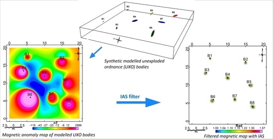
Magnetics is generally considered one of the most common and reliable methods for exploring UXO bodies. In order to avoid or minimize the danger of the blowing up of the magnetometer vehicle and/or operators, geophysical surveys with remote-control systems are recommended as they constitute proper and safer remote sensing technology. In magnetic surveying, the most important criteria are the composition (in terms of its magnetic properties), the depth, the dimensions, and the orientation of the causative body. The deeper the magnetic body, the broader will be the anomaly that is produced. UXO bodies, which are generally intensely magnetised bodies, will normally produce magnetic anomalies with large amplitudes, especially since they are usually found at relatively shallow depths. The total magnetic anomaly produced by any causative body will comprise an induced component (produced by Earth’s magnetic field interacting with the magnetic properties of the causative body) and a remanent component (produced when the causative body has its own intrinsic magnetic field because it is itself a magnet. In most cases, the induced magnetisation component dominates. In the case of UXO, however, the remanent component can be important.
The magnetic survey itself involves the systematic measurement of the total magnetic field (therefore, the induced field plus any eventual remanent field) using an instrument called a magnetometer. The sampling interval of the observation points or stations should be less than half the width of the body. Moreover, in order to determine the orientation of the body, the line spacing should be less than half the length of the body. This detectability threshold of the double of the sample spacing is called the Nyquist frequency. In other words, to reconstruct a continuous signal from a number of discrete observations, suitable for applying signal processing techniques such as those describing the edge detectors introduced above, the grid resolution should be at most half of the average spacing between the closest point pairs (e.g., the mean shortest distance) that satisfy the principles of general statistics and information theory.

4.2. Synthetic Data

A prolate (elongated) spheroid (an ellipse is rotated about its major axis) was selected for the synthetic modelling study to numerically simulate the UXO body with a simple geometric shape. This shape is the most commonly used shape for carrying out forward and inverse modelling in UXO studies [17]. The ModelVision software was used for creating the synthetic models. The synthetic dataset included the modelled responses of eight such prolate spheroid projectiles of different dimensions, depths, and orientations (both plunge and azimuth). These are shown in 3-D perspective in Figure 1, and their properties are listed in Table 1. All the bodies were assigned a magnetic susceptibility of 250 SI, and the computed measurements were made assuming a magnetic field intensity (of Earth) of 50,000 nT, with the inclination and declination being zero. The magnetic anomaly map was computed at an elevation of 1 m over the ground surface on a grid of 20 m × 20 m and grid interval of 0.05 m and is shown in Figure 2a. In order to further investigate the sensitivity of the applied techniques to detect the anomaly edges in the presence of a noise component, the originally computed data were mathematically contaminated by Gaussian random noise with a standard deviation of 0.05 of data amplitude. The computed magnetic anomaly map with superimposed random noise is shown in Figure 3a.

4.3. Magnetic Data Collected from a Test Site

A test site with the dimensions of 20 m × 20 m at the border of an artillery range in Slovakia was built by [41]. Nine Soviet tank T-34 projectiles (calibre of 100 mm) were placed on a sandy soil substrate with different longitudinal axis orientations: azimuth angle of 0° from the magnetic north, azimuth angle of 90°, and vertically plunging (in which case the azimuth angle is irrelevant). Both unfired as well as fired but unexploded projectiles (N1–N5 and F1–F4, respectively, in Figure 4) were used. The magnetic survey was conducted using a Caesium vapour magnetometer TM-4 carried by the operator with a magnetic sensor elevated 1.7 m over the ground surface, a profile interval of 1 m, and a sampling interval of 0.1 m along each profile. The data were corrected for diurnal variations, and the reference Earth’s field was subtracted from the observations in order to isolate the magnetic signatures of the ordnance. These are also seen in Figure 4.

4.4. Real Magnetic Data Collected at the Field

The magnetic surveying was carried out in an area close to a former army shooting range in Rohoznik, Slovakia [42] where several buried UXO objects can be found. The Caesium vapour magnetometer TM-4 was used to cover an area of 24 m × 100 m. The measurements were acquired along several profiles with an inline sampling interval of 0.1 m and a cross-line sampling interval of 1 m. The obtained magnetic observations were corrected for the diurnal variations, and a mean magnetic value of 48,462.8 nT, representing the magnitude of Earth’s magnetic field at the survey location, was subtracted from the corrected magnetic data in order to produce the magnetic anomaly map.

5. Results

5.1. Synthetic Data

The results of applying common edge detector processes to the magnetic data obtained from the synthetic modelling are shown in Figure 2b–h. The maximum values of the THD (Figure 2b) and AS (Figure 2c) filters clearly highlight the relatively shallow anomalous sources, but they give a wide range of positions for the more deeply buried UXO bodies. The zero contour of the TDR filter (Figure 2d), as expected, determines the edge of the subsurface magnetic source. It shows good detection results for both shallow and deeper magnetic causative bodies and does this with greater resolution than the THD and AS filters. The THD_TDR (Figure 2e) filter gave a distorted image. The Theta map (Figure 2f) and TDX (Figure 2g) filters show higher resolution images than the others with sharper edges, but these are beyond the actual positions of the boundaries of the causative bodies. The TAHG (Figure 2h) exhibits better results with edges closer to the real boundaries. It has the advantage that it can balance the edge from both shallow and deeper sources, but it also shows false anomalies. The IAS map (Figure 2i) demonstrates a higher resolution image with sharper and clearer boundaries of the shallow and deeper UXO bodies compared to other filters. Figure 3 shows the results of applying the previously mentioned edge detectors in the presence of Gaussian noise. Figure 2 and Figure 3 demonstrate the superiority of the IAS filter compared to the other commonly applied filters.

5.2. Test Site Data

The three magnetic anomaly maps for the cases observed (Figure 4) were first subjected to an upward continuation filter (up to 0.5 m) to smooth the data and reduce the effect of near-surface high-frequency structures. In addition, a reduction to the pole filter (RTP) was applied. This is a standard procedure when anomalies are expected to be dominantly induced by Earth’s magnetic field and has the effect of correcting the distortion caused by its declination and inclination at the survey location, repositioning magnetic anomalies directly above their causative sources. The RTP magnetic maps are shown in Figure 5a, Figure 6a and Figure 7a. Despite the application of the RTP filter, some anomalies still show dipolarity, which suggests the presence of a non-negligible degree of the remanent magnetism of the causative bodies.
The commonly used edge detector filters and the new IAS filter have been applied to the upward-continued RTP transformed magnetic anomalies for all three cases, and the results are presented in Figure 5, Figure 6 and Figure 7.
It can be seen that the standard filters failed to explicitly detect the UXO bodies and gave blurred, noisy images in regard to the first two cases (projectile azimuth angles of 0° and 90° from magnetic north). The case 3 (vertically plunging) results are better results, but the images remain noisy. In contrast to these, the IAS results show better resolution with the ambient magnetic signals removed, much of which can be considered as noise.

5.3. Real Field Data

The magnetic anomaly map (Figure 8a) was obtained by gridding the observed values using the Kriging interpolation algorithm over an area of 100 m by 25 m. The map suggests the presence of several interesting magnetic anomalies, but it also shows a considerable amount of “cultural” noise (metal debris, etc.). As for the test site, the observed magnetic anomaly field (Figure 8a) was first subjected to an upward continuation filter (up to 0.5 m) to smooth the data and reduce the effect of near-surface high-frequency structures and then RTP filter based on the inclination and declination of Earth’s magnetic field at the survey location. The resulting filtered RTP magnetic map (Figure 8b) is characterised by the suppression of the bipolarity of some of the anomalies and removal of high frequency cultural noise. Like the test site, there remains some dipolarity, suggesting the presence of some remanent magnetism of the causative bodies.
Figure 8c exhibits the result of applying the IAS filter to the anomaly field of Figure 5b. Six similar magnetic anomalies (A1 to A6) can be clearly distinguished on the IAS-filtered map. The peak IAS filter values for these anomalies are effectively at the upper limit of +π/2 (see colour bar), while, for other meaningful anomalies (e.g., M1 to M4), this is not the case. The presence of UXO bodies as the sources of anomalies A1 to A6 was confirmed by digging [42]. Numerous smaller metallic objects (mostly representing fragments of exploded projectiles), including those generating anomalies M1 to M4, are distributed throughout the study area, particularly in the northeast sector.

6. Discussion

A new edge detection filter has been introduced in the present study utilising the phase-based approach. The application of this filter on both synthetic and field magnetic data has demonstrated the efficiency of this edge detector in the detection of buried UXO bodies and depicting of their boundaries. The results of applying the IAS filter on magnetic data were compared with the results of applying the commonly used edge detectors, such as the THD, AS, TDR, THD_TDR, Theta map, TDX, and TAHG. Generally, these methods enhanced the magnetic anomalies associated with buried UXO bodies but with boundaries greater than the real ones (Figure 2 and Figure 3) in addition to the increase of the noise component in the resultant images (refer to Figure 3e,h). In contrast, the IAS filter was able to determine clearly and more precisely the edges of the causative sources with muted and cleaner background compared to other filters (Figure 2i, Figure 3i, Figure 4i, Figure 5i, Figure 6i and Figure 7i). Although the IAS filter obviously enhances the magnetic anomalies, it shows a slight increase of noise (Figure 3i). Therefore, the upward continuation filter was applied before applying the IAS filter. This definitely helps in suppressing the noise.
In the case of the test site, one can see that the commonly used filters produced blurred images with inaccurate boundaries (Figure 5, Figure 6 and Figure 7), whereas the IAS filter images clearly show the causative bodies with a muted background. A small shift in the locations of some of the UXO bodies can be seen on the IAS maps, which can be explained by the relatively large interval distance between the profiles compared to the size of the source bodies (refer to Figure 5i: UXOs N1, N4, and F2). The application of the THD and AS filters on these magnetic grids shows similar results, with some UXO bodies dominating, such as F1 and F4. UXO body N1 appears with faint anomalies (Figure 6b,c and Figure 7b,c). The boundaries of the UXO bodies are also generally not clear. The application of the TDR, THD_TDR, Theta map, TDX, and TAHG filters produces blurred images that are more sensitive to noise in addition to the generation of false edges (for example, Figure 6f,g and Figure 7f,g). On the other hand, the IAS filter outlines the boundaries of the UXO bodies in a better way compared to the commonly used filters without producing any false edges.
Figure 8 demonstrates the most important results. The UXO bodies producing anomalies (A1–A6) were precisely detected despite the noisy natural environment. Moreover, despite the overlapping of anomalies A1 and A2 in the observed magnetic field, the IAS filter was able to define the locations of their causative sources successfully. Furthermore, the application of upward continuation and choosing the range (1 – π/2) for the IAS filter leads to obtaining a clear image with less noise. Unlabelled circular anomalies in Figure 8c, such as those located at (6.3, 50), (18, 71) and (14, 86), can also be interpreted as UXO of small sizes or parts of UXO bodies. Other small anomalies appearing in Figure 8c probably represent metallic materials located at shallow depths (for example, fragments of UXO bodies). The presence of such materials in a survey area may complicate the discrimination process, which can be one of the drawbacks of the introduced filter.
Nevertheless, the discrimination between the causative sources (UXOs) and other metallic materials in the subsurface is one of the advantages of the IAS filter. Anomaly M1 (Figure 8c) is generated by a horizontally lying iron non-UXO body on the surface, and the anomalies labelled M2–M4 are probably the result of similar non-UXO ferrous, magnetic objects. This reflects the effectiveness of the IAS filter in the discrimination between UXOs and non-UXO metallic materials, which leads, in turn, to reducing the false alarms generated by fragments of UXO and other metallic clutter. However, some synthetic modelling studies and/or field experiments for the discrimination of UXO and non-UXO materials using the IAS filter should be considered as worthy of further research.

7. Conclusions

A new phase-based filter called IAS (improved analytical signal) has been introduced for the fast and precise detection and locating of UXO bodies. The IAS filter has been tested on noise-free and noisy synthetic magnetic data as well as on magnetic data collected in the field. The efficiency and validation of the new filter were compared with other known edge detectors using these synthetic and real magnetic data. The IAS edge detector shows better results in the detection of the buried UXO objects for both weak and strong anomalies and also for shallow and deep targets. It also demonstrates the ability to discriminate UXO bodies from other metallic materials.
Parallel to the continuous efforts aimed at the disposal of UXO bodies, it remains urgent to find the optimal manner to save the lives of innocent civilians in areas of conflict. Awareness programmes about the risk of explosive materials by national and international organisations are essential and of great importance.

Author Contributions

Conceptualization, I.M.I. and H.A.; methodology, I.M.I. and M.F.A.; software, I.M.I. and R.S.; validation, I.M.I., H.A. and M.F.A.; formal analysis, I.M.I.; investigation, I.M.I. and M.F.A.; resources, H.A. and I.M.I.; data curation, I.M.I.; writing—original draft preparation, I.M.I., H.A. and M.F.A.; writing—review and editing, I.M.I. and R.S.; visualization, I.M.I.; supervision, R.S.; project administration, R.S.; funding acquisition, H.A., I.M.I. and M.F.A. All authors have read and agreed to the published version of the manuscript.

Funding

This research was funded by the Council for at-Risk Academics (CARA), United Kingdom. The grant was awarded under the CARA Syria programme, grant award number Jul19LGURN17.

Data Availability Statement

The data used to support the findings of this study are available from the corresponding author upon reasonable request.

Acknowledgments

The authors are grateful to the Cara (Council for At-Risk Academics) for supporting this research. We also thank Roman Pašteka and Valeria Paoletti for providing us the magnetic data used in this study and for their constructive and fruitful discussion. The G-trend Ltd. company is highly acknowledged for the permission to use the magnetic data of the Rohoznik site.

Conflicts of Interest

The authors declare no conflict of interest.

References

  1. SNHR. Syrian Network for Human Rights Report. 2020, p. 17. Available online: https://sn4hr.org/wp-content/pdf/english/Syria_Is_Among_the_Worlds_Worst_Countries_for_the_Number_of_Mines_Planted_Since_2011_en.pdf (accessed on 25 May 2021).
  2. Czub, M.; Kotwicki, L.; Lang, T.; Sanderson, H.; Klusek, Z.; Grabowski, M.; Szubska, M.; Jakacki, J.; Andrzejewski, J.; Rak, D.; et al. Deep Sea habitats in the chemical warfare dumping areas of the Baltic Sea. Sci. Total Environ. 2018, 616-617, 1485–1497. [Google Scholar] [CrossRef] [PubMed]
  3. Klammler, H.; Sheremet, A.; Calantoni, J. Seafloor Burial of Surrogate Unexploded Ordnance by Wave-Induced Sediment Instability. IEEE J. Ocean. Eng. 2020, 45, 927–936. [Google Scholar] [CrossRef]
  4. Salem, A.; Hamada, T.; Asahina, J.K.; Ushijima, K. Detection of unexploded ordnance (UXO) using marine magnetic gradiometer data. Explor. Geophys. 2005, 36, 97–103. [Google Scholar] [CrossRef]
  5. Billings, S.D.; Li, Y.; Goodrich, W. Advanced UXO Discrimination Using Magnetometry—Understanding Remanent Magnetization: Final Report SERDP Project MM-1380; Strategic Environmental Research and Development Program; Sky Research, Inc.: Alexandria, VA, USA, 2009; Available online: https://serdp-estcp.org/index.php//Program-Areas/Munitions-Response/Land/Modeling-and-Signal-Processing/MR-1380.
  6. Billings, S.; Youmans, C. Experiences with unexploded ordnance discrimination using magnetometry at a live-site in Montana. J. Appl. Geophys. 2007, 61, 194–205. [Google Scholar] [CrossRef]
  7. Davis, K.; Li, Y.; Nabighian, M. Automatic detection of UXO magnetic anomalies using extended Euler deconvolution. SEG Tech. Program. Expanded Abstr. 2005, 1133–1136. [Google Scholar] [CrossRef] [Green Version]
  8. Wigh, M.; Hansen, T.M.; Døssing, A. Inference of Unexploded Ordnance (UXO) by Probabilistic Inversion of Magnetic Data. Geophys. J. Int. 2020, 220, 37–58. [Google Scholar] [CrossRef] [Green Version]
  9. Reynolds, R.; Barrowes, B.; Shubitidze, T.; Hartshorn, C.; Quinn, B.; Shubitidze, F. Electromagnetic induction sensing of unexploded ordinance and soil properties from unmanned aerial systems. In Proceedings of the SPIE 11750, Detection and Sensing of Mines, Explosive Objects, and Obscured Targets XXVI, Online, 12–17 April 2021; p. 1175002. [Google Scholar] [CrossRef]
  10. O’Neill, K.; Fernández, J.B. Electromagnetic Methods for UXO Discrimination. In Unexploded Ordnance Detection and Mitigation; Byrnes, J., Ed.; Springer: Dordrecht, The Netherlands, 2009; pp. 197–221. [Google Scholar]
  11. Zhao, Y.; Xu, F.; Liu, J. Transient electromagnetic detection of unexploded ordnance buried in underwater sediments. In Proceedings of the OCEANS 2018 MTS/IEEE Charleston, Charleston, SC, USA, 22–25 October 2018; pp. 1–5. [Google Scholar] [CrossRef]
  12. Brito-da-Costa, A.M.; Martins, D.; Rodrigues, D.; Fernandes, L.; Moura, R.; Madureira-Carvalho, Á. Ground Penetrating Radar for Buried Explosive Devices Detection: A Case Studies Review. Aust. J. Forensic Sci. 2021, 1–20. [Google Scholar] [CrossRef]
  13. Daniels, D.J. Ground Penetrating Radar for Buried Landmine and IED Detection. In Unexploded Ordnance Detection and Mitigation; Springer: Dordrecht, The Netherlands, 2009; pp. 89–111. [Google Scholar]
  14. Griffiths, H.; McAslan, A. Low Frequency Radar for Buried Target Detection. In Unexploded Ordnance Detection and Mitigation; Byrnes, J., Ed.; Springer: Dordrecht, The Netherlands, 2009; pp. 125–140. [Google Scholar]
  15. Núñez-Nieto, X.; Solla, M.; Gómez-Pérez, P.; Lorenzo, H. GPR Signal Characterization for Automated Landmine and UXO Detection Based on Machine Learning Techniques. Remote Sens. 2014, 6, 9729–9748. [Google Scholar] [CrossRef] [Green Version]
  16. Beran, L.; Zelt, B.; Billings, S.D. Detecting and classifying UXO. J. ERW Mine Action 2013, 17, 57–63. [Google Scholar]
  17. Butler, D.K.; Simms, J.E.; Furey, J.S.; Bennett, H.H. Review of Magnetic Modeling for UXO and Applications to Small Items and Close Distances. J. Environ. Eng. Geophys. 2012, 17, 53–73. [Google Scholar] [CrossRef]
  18. Reynolds, J.M.A. Introduction to Applied and Environmental Geophysics, 2nd ed.; John Wiley and Sons: Hoboken, NJ, USA, 2011. [Google Scholar]
  19. Wu, G.; Huang, D.; Zhang, C.; Yuan, Y. Detection of UXO magnetic anomaly in Jinshan area. Glob. Geology 2015, 18, 54–58. [Google Scholar]
  20. Nelson, H.H.; Altshuler, T.W.; Rosen, E.M.; McDonald, J.R.; Barrow, B.; Khadr, N. Magnetic modeling of UXO and UXO-like targets and comparison with signatures measured by MTADS. In Proceedings of the UXO Forum, Anaheim, CA, USA, 19 May 1998; pp. 282–291. [Google Scholar]
  21. Butler, D.K. Potential fields methods for location of unexploded ordnance. Leading Edge 2001, 20, 890–895. [Google Scholar] [CrossRef]
  22. Billings, S.; Pasion, L.; Oldenburg, D. Discrimination and Identification of UXO by Geophysical Inversion of Total-Field Magnetic Data: ERDC/GSL TR-02-16; US Army Engineer Research and Development Center: Vicksburg, MS, USA, 2002.
  23. Paoletti, V.; Buggi, A.; Pašteka, R. UXO Detection by Multiscale Potential Field Methods. Pure Appl. Geophys. 2019, 176, 4363–4381. [Google Scholar] [CrossRef]
  24. Appiah, I.; Wemegah, D.D.; Asare, V.-D.S.; Danuor, S.K.; Forson, E.D. Integrated geophysical characterisation of Sunyani Municipal solid waste disposal site using magnetic gradiometry, magnetic susceptibility survey and electrical resistivity tomography. J. Appl. Geophys. 2018, 153, 143–153. [Google Scholar] [CrossRef]
  25. Benson, R.; Glaccum, R.A.; Noel, M.R. Geophysical Techniques for Sensing Buried Wastes and Waste Migration; National Ground Water Association: Westerville, OH, USA, 1982; pp. 163–188. [Google Scholar]
  26. Dumont, G.; Robert, T.; Mark, N.; Nguyen, F. Assessment of multiple geophysical techniques for the characterization of municipal waste deposit sites. J. Appl. Geophys. 2017, 145, 74–83. [Google Scholar] [CrossRef]
  27. Ibraheem, I.M.; Tezkan, B.; Bergers, R. Integrated interpretation of magnetic and ERT data to characterize a landfill in the north-west of Cologne, Germany. Pure Appl. Geophys. 2021, 178, 2127–2148. [Google Scholar] [CrossRef]
  28. Soupios, P.; Ntarlagiannis, D. Characterization and monitoring of solid waste disposal sites using geophysical methods: Current applications and novel trends. In Modelling Trends in Solid and Hazardous Waste Management; Sengupta, D., Agrahari, S., Eds.; Springer: Singapore, 2017; pp. 75–103. [Google Scholar]
  29. Wemegah, D.D.; Fiandaca, G.; Auken, E.; Menyeh, A.; Danour, S.K. Spectral time-domain induced polarization and magnetics surveying– an efficient tool for characterisation of solid waste deposits in developing countries. Near Surf. Geophys. 2017, 15, 75–84. [Google Scholar] [CrossRef] [Green Version]
  30. Ibraheem, I.M.; Gurk, M.; Tougiannidis, N.; Tezkan, B. Subsurface imaging of the Neogene Mygdonian basin, Greece using magnetic data. Pure Appl. Geophys. 2018, 175, 2955–2973. [Google Scholar] [CrossRef]
  31. Ibraheem, I.M.; Haggag, M.; Tezkan, B. Edge Detectors as Structural Imaging Tools Using Aeromagnetic Data: A Case Study of Sohag Area, Egypt. Geosciences 2019, 9, 211. [Google Scholar] [CrossRef] [Green Version]
  32. Cordell, L.; Grauch, V.J.S. Mapping basement magnetization zones from aeromagnetic data in the San Juan basin, New Mexico. In The Utility of Regional Gravity and Magnetic Anomaly Maps; Hinzc, W.J., Ed.; Society of Exploration Geophysicists: Tulsa, OK, USA, 1985; pp. 181–197. [Google Scholar]
  33. Roest, W.R.; Verhoef, J.; Pilkington, M. Magnetic interpretation using the 3-D analytic signal. Geophysics 1992, 57, 116–125. [Google Scholar] [CrossRef]
  34. Miller, H.G.; Singh, V. Potential field tilt—A new concept for location of potential field sources. J. Appl. Geophys. 1994, 32, 213–217. [Google Scholar] [CrossRef]
  35. Verduzco, B.; Fairhead, J.D.; Green, C.M.; MacKenzie, C. New insights into magnetic derivatives for structural mapping. Lead. Edge 2004, 23, 116–119. [Google Scholar] [CrossRef]
  36. Wijns, C.; Perez, C.; Kowalczyk, P. Theta map: Edge detection in magnetic data. Geophysics 2005, 70, L39–L43. [Google Scholar] [CrossRef]
  37. Cooper, G.R.J.; Cowan, D.R. Enhancing potential field data using filters based on the local phase. Comp. Geosci. 2006, 32, 1585–1591. [Google Scholar] [CrossRef]
  38. Ferreira, F.; De Souza, J.; Bongiolo, A.D.B.E.S.; De Castro, L.G. Enhancement of the total horizontal gradient of magnetic anomalies using the tilt angle. Geophysics 2013, 78, J33–J41. [Google Scholar] [CrossRef]
  39. Nabighian, M.N. The analytic signal of two-dimensional magnetic bodies with polygonal cross-section: Its properties and use for automated anomaly interpretation. Geophysics 1972, 37, 507–517. [Google Scholar] [CrossRef]
  40. Li, X. Understanding 3D analytic signal amplitude. Geophysics 2006, 71, L13–L16. [Google Scholar] [CrossRef]
  41. Pašteka, R.; Mikuška, J.; Karcol, R. New Methods in Ammunition Detection; Report PPZ-VTR-69-015/2010, MS; G-trend Ltd.: Bratislava, Slovakia, 2008; pp. 1–14. (In Slovak) [Google Scholar]
  42. Mikuška, J.; Pašteka, R.; Hajach, M.; Kadeckŷ, J.; Appel, J. Pyrotechnical Exploration along Planned Seismic Reflection Profile trough the Military Site Zahorie; Technical Report; G-trend Ltd. and Pyra Ltd.: Bratislava, Slovakia, 2006; pp. 1–2. (In Slovak) [Google Scholar]
Figure 1. 3-D perspective of 8 synthetic modelled unexploded ordnance (UXO) bodies within a grid of 20 m × 20 m. The UXO modelled bodies have different dimensions, azimuths, and plunges and are located at different depths, up to a maximum of 4 m.
Remotesensing 13 04345 g001
Figure 2. (a) Synthesised magnetic anomaly map of model causative bodies (Figure 1; Table 1) calculated at height of 1 m from the ground. Filtered maps of (a) with the indicated edge detectors applied (b) total horizontal gradient (THD), (c) analytical signal (AS), (d) tilt angle derivative filter (TDR), (e) THD_TDR, (f) Theta map, (g) horizontal tilt angle (TDX), (h) tilt angle of the horizontal derivative amplitude (TAHG), and (i) IAS (edge detector developed in this study).
Remotesensing 13 04345 g002
Figure 3. (a) Synthesised magnetic anomaly map of model causative bodies (Figure 1; Table 1) contaminated with Gaussian random noise with a standard deviation of 5% of the data amplitude. Filtered maps of (a) with the indicated edge detectors applied (b) THD, (c) AS, (d) TDR, (e) THD_TDR, (f) Theta map, (g) TDX, (h) TAHG, and (i) IAS. The effects of noise contamination of this magnitude are minor but most evident in (e,h,i).
Remotesensing 13 04345 g003
Figure 4. Photos and 20 m × 20 m magnetic maps produced by unfired (N1–N5) as well as fired but unexploded (F1–F4) projectiles with different orientations: (a) horizontally with azimuth of 0°, (b) horizontally with azimuth of 90°, and (c) vertically with the tip pointing downward.
Remotesensing 13 04345 g004
Figure 5. (a) Upward continued reduction to the pole filter (RTP) magnetic anomaly map from the test site, case 1, with filters applied as follows: (b) THD, (c) AS, (d) TDR, (e) THD_TDR, (f) Theta map, (g) TDX, (h) TAHG, and (i) IAS.
Remotesensing 13 04345 g005
Figure 6. (a) Upward continued RTP magnetic anomaly map from the test site, case 2, with filters applied as follows: (b) THD, (c) AS, (d) TDR, (e) THD_TDR, (f) Theta map, (g) TDX, (h) TAHG, and (i) IAS.
Remotesensing 13 04345 g006
Figure 7. (a) Upward continued RTP magnetic anomaly map from the test site, case 3, with filters applied as follows: (b) THD, (c) AS, (d) TDR, (e) THD_TDR, (f) Theta map, (g) TDX, (h) TAHG, and (i) IAS.
Remotesensing 13 04345 g007
Figure 8. (a) Magnetic anomaly map (100 m × 25 m) of the surveyed area in Rohoznik, Slovakia, (b) 1.5 m upward continued magnetic anomaly map of the studied site, and (c) IAS map of the magnetic data where six magnetic anomalies produced by UXO (A1 to A6) can be seen in addition to several other anomalies attributed to other metallic materials.
Remotesensing 13 04345 g008
Table 1. Parameters of synthetic modelled unexploded ordnance (UXO) bodies.
UXO
Body
X
(m)
Y
(m)
Depth
(m)
Length/2
(m)
Diameter/2
(m)
AzimuthPlungeSusc.
(SI)
Type
1517.50.350.240.05233045250105 mm projectile
21516.50.550.4350.087030250175 mm projectile
3413.50.800.6050.152454525012 in projectile
410121.100.8450.203300025016 in projectile
516101.000.7950.13328010250500 lb bomb
6661.501.2500.22945602501000 lb bomb
71261.200.9200.170002502000 lb bomb
817410.8450.203300025016 in projectile
Publisher’s Note: MDPI stays neutral with regard to jurisdictional claims in published maps and institutional affiliations.

