Article

Hyperspectral Image Classification Based on Two-Branch Spectral–Spatial-Feature Attention Network

1
College of Astronautics, Nanjing University of Aeronautics and Astronautics, Nanjing 210016, China
2
Key Laboratory of Space Photoelectric Detection and Perception, Ministry of Industry and Information Technology, Nanjing University of Aeronautics and Astronautics, Nanjing 210016, China
3
National Key Laboratory Science and Technology Space Microwave, China Academic Space Technology, Xi’an 710018, China
4
Control Science and Engineering, Harbin Institute of Technology, Harbin 150001, China
*
Author to whom correspondence should be addressed.
Remote Sens. 2021, 13(21), 4262; https://doi.org/10.3390/rs13214262
Submission received: 14 September 2021 / Revised: 15 October 2021 / Accepted: 20 October 2021 / Published: 23 October 2021
(This article belongs to the Special Issue Recent Advances in Hyperspectral Image Processing)

Abstract

:
Although most of deep-learning-based hyperspectral image (HSI) classification methods achieve great performance, there still remains a challenge to utilize small-size training samples to remarkably enhance the classification accuracy. To tackle this challenge, a novel two-branch spectral–spatial-feature attention network (TSSFAN) for HSI classification is proposed in this paper. Firstly, two inputs with different spectral dimensions and spatial sizes are constructed, which can not only reduce the redundancy of the original dataset but also accurately explore the spectral and spatial features. Then, we design two parallel 3DCNN branches with attention modules, in which one focuses on extracting spectral features and adaptively learning the more discriminative spectral channels, and the other focuses on exploring spatial features and adaptively learning the more discriminative spatial structures. Next, the feature attention module is constructed to automatically adjust the weights of different features based on their contributions for classification to remarkably improve the classification performance. Finally, we design the hybrid architecture of 3D–2DCNN to acquire the final classification result, which can significantly decrease the sophistication of the network. Experimental results on three HSI datasets indicate that our presented TSSFAN method outperforms several of the most advanced classification methods.

Graphical Abstract

1. Introduction

Hyperspectral imagery is captured with the spectrometer and supplies rich spectral information containing tens to hundreds of narrow bands for all the image elements [1,2,3]. Hyperspectral image (HSI) contains rich features of ground [4,5,6], in which spatial features and spectral features are both included for each pixel. As a result, it is utilized widely in multiple fields of agriculture [7], target detection [8], environmental monitoring [9], urban planning [10], and military reconnaissance [11]. In these applications, the classification of HSI [12,13,14,15] is a basic problem, which aims to find the specific class of each pixel.
Over the past few decades, diverse classification methods have been proposed to tackle this challenge, such as support vector machines (SVM) [16], k-nearest neighbor (KNN) [17], random forests [18], and multinomial logistic regression (MLR) [19], etc. However, these methods mentioned above have a common disadvantage that they classify the pixel by only applying the spectral information. While the spectral information of the pixel belonging to one category is very likely mixed with the spectral information of pixels from other categories. Therefore, these classification methods mentioned above, which have obvious shortcomings, are not robust to noise, and their classification results do not always perform well.
To solve such problems, various novel classification methods have been introduced in the past several years, which try to improve the classification performance by incorporating spatial information. One category in these methods attempts to design diverse feature extraction approaches, including the local binary pattern (LBP) histogram feature extraction [20] and extended morphological profiles (EMP) extraction [21], etc. The disadvantage of this type of method is that they extract only a single feature, so the improvement of classification performance is limited. The other tries to fuse spectral information with spatial contexts by adopting the joint sparse representation classification (JSRC) model [22]. The representative methods include: space-spectrum combined kernel filter [23], multiple kernel sparse representation classifier with superpixel features [24], kernel sparse representation-based classification (KSRC) method [25], and so on. Although these methods perform better on the specific datasets, they show the disadvantage that the designed classification models are more complex and less adaptable. Compared with the methods that only use spectral information, these methods can effectively enhance the classification performance. However, all these classification methods mentioned above design and extract features based on specific data with different structures. They have no universality for diverse hyperspectral datasets and cannot simultaneously achieve good results for data with different structures.
Therefore, researchers gradually introduce deep-learning mechanisms [26,27,28,29,30] to replace the methods of manually extracting features, which can automatically design feature extraction and solve various problems caused by the diversification of hyperspectral data structures. Chen [31] first applies the deep-learning network SAE to the HSI classification and proposes a deep-learning model that fuses spectral features and spatial features to obtain high classification accuracy. Then, more and more deep-learning models [32,33,34,35] are explored by researchers. Zhao [36] introduces the deep belief network (DBN) model into the HSI classification, and the data are preprocessed to decrease the redundancy by the principal component analysis (PCA) method. The hierarchical learning of features and the use of logistic regression methods to extract the spatial spectrum feature can achieve good experimental results. Wei [37] first applies the convolutional neural network (CNN) to the HSI classification, but the established CNN model can only extract spectral features. Chen [38] proposes a CNN-based depth feature extraction method, which establishes a three-dimensional convolutional neural network, so that the spatial and spectral features can be extracted, meanwhile. Zhong [39] proposes the spectral–spatial residual network (SSRN), which facilitates the back propagation of the gradient, while extracting deeper spectral features and alleviating that the accuracy of other deep-learning models is reduced. Sellami [40] introduces the semi-supervised three-dimensional CNN into the HSI classification through adaptive dimensionality reduction to solve the dimensionality curse problem. Mei [41] proposes the spectral–spatial attention network and achieves a good training result with the incorporation of attention mechanism into their model. Despite the competitive classification performance being achieved by the above deep-learning-based approaches, they still remain two major disadvantages. One is that the training samples are massively required for the purpose of learning the parameters in the deep network. However, expensive economic costs and a lot of time must be spent in order to collect such labelled data, which directly results in a very limited quantity of labelled data in practical applications. The other is that the neural network needs to adjust numerous variables during the backpropagation, which results in considerable calculation costs and time costs. Therefore, it remains a challenge to utilize small-size training samples to concurrently extract discriminative spectral–spatial features and remarkably enhance the classification performance.
In this paper, a novel two-branch spectral–spatial-feature attention network (TSSFAN) for HSI classification is proposed. Firstly, two inputs with different spectral dimensions and spatial sizes are constructed for the network, which can not only reduce the redundancy of the original dataset but also accurately and separately explore the spectral and spatial features. Then, two parallel 3DCNN branches with attention modules are designed for the network, in which one focuses on extracting spectral features and adaptively learning the more discriminative spectral channels, and the other focuses on exploring spatial features and adaptively learning the more discriminative spatial structures. Next, the feature attention module is constructed in the fusion stage of the two branches to automatically adjust the weights of different features based on their contributions for the classification. Finally, the 2DCNN network is designed to obtain the final classification result, which can decrease the sophistication of the network and reduce the parameters in the network. Compared with several typical and recent HSI classification methods, the results indicate that our presented TSSFAN is superior to the most advanced methods.
The remaining chapters of the article are organized as follows. The CNN network, attention mechanism, and the proposed TSSFAN method are introduced in Section 2. The classification results of three different public datasets are presented in Section 3. The article is concluded in Section 4, finally.

2. Materials and Methods

In this section, the traditional methods including 2DCNN, 3DCNN, and attention mechanism are the first to be introduced. Then, the process of the proposed TSSFAN method is explained in detail.

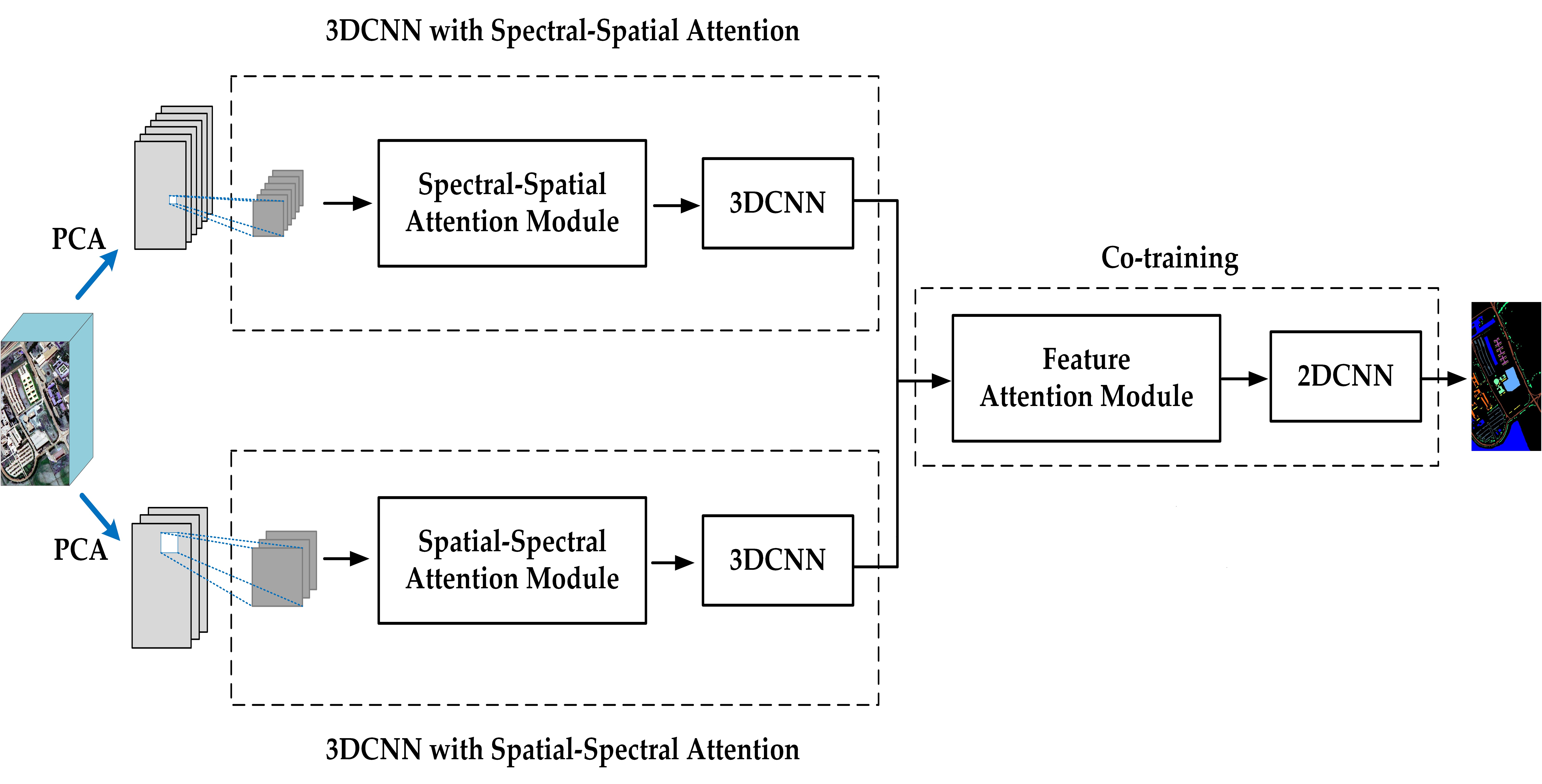
2.1. 2DCNN and 3DCNN

Convolutional neural network (CNN) [42,43,44,45] is commonly employed in the computer vision (CV) task. Inspired by the thinking mode of the human brain, CNN can automatically learn the spatial features of images by the convolution and pooling operations [46,47,48,49,50], which contains multiple layers of repetitive stacked structures to extract deep information. CNN is originally designed for the recognition of two-dimensional images, so the traditional network structure is a two-dimensional convolutional neural network [51,52,53]. A typical 2DCNN structure is presented in Figure 1.
In the convolution layer, the convolution kernel is first used to perform convolutional operations on the input image. Then, the convolutional result is fed into a nonlinear function, and its output is sent to the next layer for further computation. Different from the fully connected neural network (FC), the training parameters in CNN are remarkably reduced due to the application of the shared convolution kernel. The convolution formula is as follows:
F l = f ( F l 1 W l + b l )
where f ( ) indicates the nonlinear activation function, and it can strengthen the network’s ability to process nonlinear data. F l 1 is the input feature map in layer l 1 , and F l is the output feature map in layer l . W l indicates the convolutional filter, and b l indicates the bias of each output feature map.
In the pooling layers, the previous feature maps are sub-sampled to reduce the spatial size. After the multilayer architectures are stacked, the fully connected layer and the SoftMax classifier are typically utilized to present the final results.
Although 2DCNN can recognize two-dimensional shapes very well, it does not perform satisfactorily when directly processing three-dimensional data. Therefore, 2DCNN is promoted to 3DCNN to extract high-level 3D features [54] for three-dimensional data. Figure 2 presents a typical 3DCNN structure. It has a highly similar structure with 2DCNN, but their difference is that 2DCNN uses the 2D convolution kernel, while 3DCNN uses the 3D convolution kernel. Three-dimensional CNN [55,56,57,58] can simultaneously extract spatial and depth features for three-dimensional data via the 3D convolution kernel.

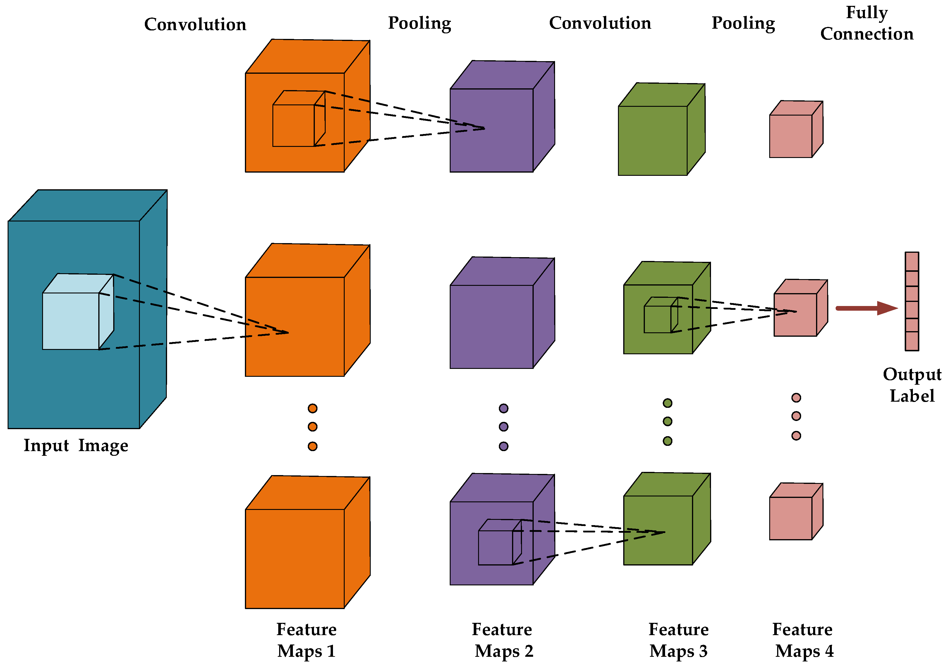
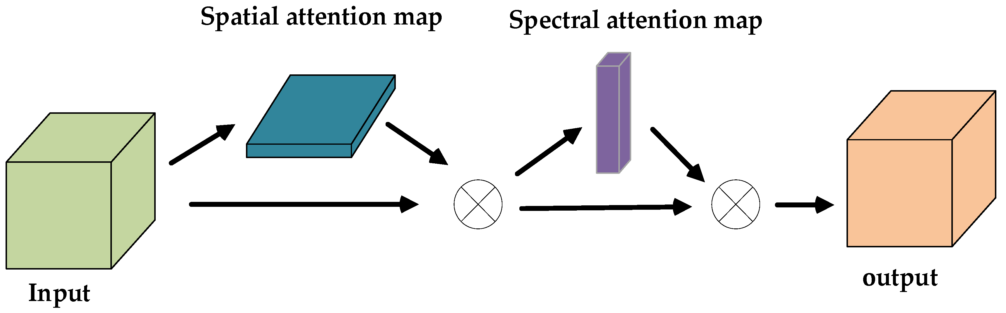
2.2. Attention Mechanism

As the applications of deep learning in many CV tasks become more and more extensive, attention mechanism [59,60,61] as an auxiliary means is increasingly used in deep networks to optimize the network structure. Attention mechanism [62] is similar to the way that the human eyes observe things, which can always ignore the irrelevant information but pay attention to the significant information. It makes the network focus on learning [63], which can remarkably enhance the performance of the network. Figure 3 presents a typical attention module.
As can be seen from Figure 3, the attention module aims to construct an adaptive function, which maps the original images to the matrix that represents the weights of different spatial locations. With the help of such a function, different regions are given independent weights to highlight more relevant and noteworthy information. The process can be expressed by:
Y = F s a a t t e n t i o n ( s i g m o d ( ( F m a x , F a v g ) W + b ) , X )
where X is the original image, while Y indicates the output. F m a x indicates maximum pooling along the channel dimension, while F a v g represents average pooling along the channel dimension. W , b indicate the convolutional filter and the bias in the convolutional operation, respectively. X s is the generated weight matrix, and F s a a t t e n t i o n ( ) indicates spatial-wise multiply between the original input X and weight X s .

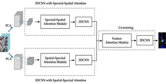
2.3. Proposed TSSFAN Method

Figure 4 depicts the flowchart of the proposed method TSSFAN. From this flowchart, the TSSFAN method has four main steps: data preprocessing, two-branch 3DCNN with attention modules, feature attention module in the co-training model, and 2DCNN for classification. Next, each main step of the TSSFAN method is introduced in detail.

2.3.1. Data Preprocessing

Let the HSI dataset be denoted by I R H × W × C , where I represents the original input; H , W , C indicate the height, the width, and channel numbers of I . The steps of data preprocessing are described as follows, and Figure 5 shows the process.
(1)
PCA is employed to reduce the spectral dimension of the original image and obtain two datasets with different spectral dimensions, where P H × W × D 1 and Q H × W × D 2 .
(2)
Based on the two different spectral dimensions, the image with the larger spectral dimension selects a smaller spatial window to create an input 3D cube for each center pixel, while the image with the smaller spectral dimension selects a larger spatial window to create another input 3D cube for each center pixel, where Input_1 is denoted by U M × M × D 1 and Input_2 is denoted by V N × N × D 2 , respectively.
Through such data preprocessing, we create two inputs with different spectral dimensions and spatial sizes, which can not only reduce the redundancy of the original dataset but also accurately and separately explore the spectral and spatial features.

2.3.2. Two-Branch 3DCNN with Attention Modules

After data preprocessing, two inputs with different spectral dimensions and spatial sizes are obtained. Then, we design two parallel 3DCNN branches, where each branch contains an attention module. One branch focuses on spatial feature extraction, and the other focuses on spectral feature extraction. Moreover, the attention module in each branch can automatically adjust the weights of the spatial features and spectral features for different input data, concentrating on more discriminative spatial structures and spectral channels.
  • 3DCNN with Spectral–Spatial Attention
For Input_1 U M × M × D 1 with the larger spectral dimension, we design a branch of 3DCNN with spectral–spatial attention, which focuses on extracting spectral features and adaptively learning the more discriminative spectral channels. Figure 6 shows the process. Below, the two main steps of this branch are presented in detail.
Step 1: Let Input_1 U M × M × D 1 pass through the spectral–spatial attention module, which can automatically adjust the weights of the spectral features and the spatial features for different input data, concentrating on more discriminative spectral channels and spatial structures. Specifically, Figure 7 presents the spectral–spatial attention module.
As can be seen from Figure 7, let the input be denoted by Y H × W × C , where H , W , C indicate the height, the width, and channel numbers of Y . Let the spectral attention map be denoted by A s e 1 × 1 × C , the spatial attention map be denoted by A s a H × W × 1 , and the output be denoted by Y e a H × W × C . The computation process can be denoted as:
Y e a = F s a a t t e n t i o n ( F s e a t t e n t i o n ( Y , A s e ) , A s a )
where Y e a is the output. F s e a t t e n t i o n ( ) , F s a a t t e n t i o n ( ) represent the spectral-wise multiply and spatial-wise multiply, respectively.
In the spectral–spatial attention module, the acquisition of the spectral attention map and the spatial attention map are two necessary parts. Additionally, the process of obtaining the spectral attention map and the spatial attention map is as follows.
(a)
Spectral attention map:
The spectral attention exploits the inter-channel relationships of feature maps and aims to construct an adaptive function, which maps the original images to the vector that represents the weights of different spectral bands. As can be seen from Figure 8a, the global average pooling and the global max pooling are first operated to squeeze the spatial dimension to obtain the Avg-Pool Y c a v g 1 × 1 × C and Max-Pool Y c m a x 1 × 1 × C , respectively. Then, the Avg-Pool and Max-Pool are passed through two fully connected layers with shared parameters. Finally, the two outputs are added and passed through the sigmoid function to obtain the spectral attention map. The process is calculated as follows:
A s e = σ ( f ( f ( Y c a v g W 1 + b 1 ) W 2 + b 2 ) + f ( f ( Y c m a x W 1 + b 1 ) W 2 + b 2 ) )
where Y c a v g , Y c m a x indicate the feature map obtained by the global average pooling and the global max pooling, respectively. W 1 , b 1 are the parameter of the first fully connected layer, and W 2 , b 2 indicate the parameter of the second fully connected layer. f ( ) denotes the ReLU function, and σ is the sigmoid function.
(b)
Spatial attention map:
The spatial attention aims to construct an adaptive function, which maps the original images to the matrix that represents the weights of different spatial locations. From Figure 8b, the global average pooling and the global max pooling are first operated along the channel direction, squeezing the spectral dimension to obtain the Avg-Pool Y a v g H × W × 1 and Max-Pool Y m a x H × W × 1 , respectively. Next, we concatenate the Avg-Pool and Max-Pool, then, pass them through a 2D convolutional layer. At last, the spatial attention map A s a is generated with the application of a sigmoid function. The process is calculated as follows:
A s a = σ ( ( Y a v g , Y max ) W 3 + b 3 )
where Y a v g , Y max indicate the feature map obtained by the global average pooling and the global max pooling, respectively. W 3 , b 3 are the parameter of the 2D convolutional layer. Additionally, σ is the sigmoid function.
Step 2: As can be seen from Figure 6, two 3D convolutional layers are employed to extract spectral and spatial features simultaneously after passing through the spectral–spatial attention module. Finally, output 1 with size { S × S × C , P } is obtained. In the 3D convolution, the convolution formula is calculated by:
F l = R e l u ( F l 1 W l + b l )
where F l 1 is the input feature map in layer l 1 , and F l is the output feature map in layer l . W l indicates the 3D convolutional filter, and b l indicates the bias of each output feature map. R e l u ( ) is the nonlinear activation function.
B.
3DCNN with Spatial–Spectral Attention
For Input_2 V N × N × D 2 with the larger spatial size, we design a branch of 3DCNN with spatial–spectral attention, which focuses on exploring spatial features and adaptively learning the more discriminative spatial structures. Figure 9 shows the process. The two branches are very similar, and the main difference is that they use different attention modules, which are the spectral–spatial attention module presented in Figure 7 and the spatial–spectral attention module presented in Figure 10, respectively. By comparing Figure 7 and Figure 10, we can see that the spectral–spatial attention module prioritizes spectral attention before spatial attention, while the spatial–spectral attention module is just the opposite. The reason for this design is that the Input_1 U M × M × D 1 contains more spectral information so spectral attention is given priority, while Input_2 V N × N × D 2 contains more spatial information so spatial attention is given priority.
Finally, through the similar structure, output 2 with size { S × S × C , P } is also obtained. The size of the output in both branches is the same, because we acquire the output with the same size by controlling the convolution operation, so that the output of the two branches can be merged later.

2.3.3. Feature Attention Module in the Co-Training Model

As shown in Figure 11, the next step is to concatenate the two branches for co-training. The outputs of the two 3DCNN branches are merged together, and we obtain the output with size { S × S × C , 2 P }. We consider that different features from different branches do not contribute equally to the classification task. If we can fully explore the prior information, then, the learning ability of the entire network will be improved to a considerable extent. Therefore, we construct the feature attention module to automatically adjust the weights of different features based on their contributions for classification, which can remarkably enhance the classification performance. Figure 12 presents the feature attention module.
In the feature attention module, for the input X i S × S × C × 2 P , the global average pooling and the global max pooling are operated in the direction of the channel to obtain the global feature description maps, i.e., F a v g 1 × 1 × 1 × 2 P and F m a x 1 × 1 × 1 × 2 P . The weight X w 1 × 1 × 1 × 2 P of different features is obtained through a structure similar to the spectral attention map. Finally, the output X j S × S × C × 2 P is calculated as
X j = X i X w
where indicates the channel-wise multiplication.
By the constructed feature attention module, different features are given different weights based on their contributions for the classification task. We acquire the output with size { S × S × C , 2 P }.

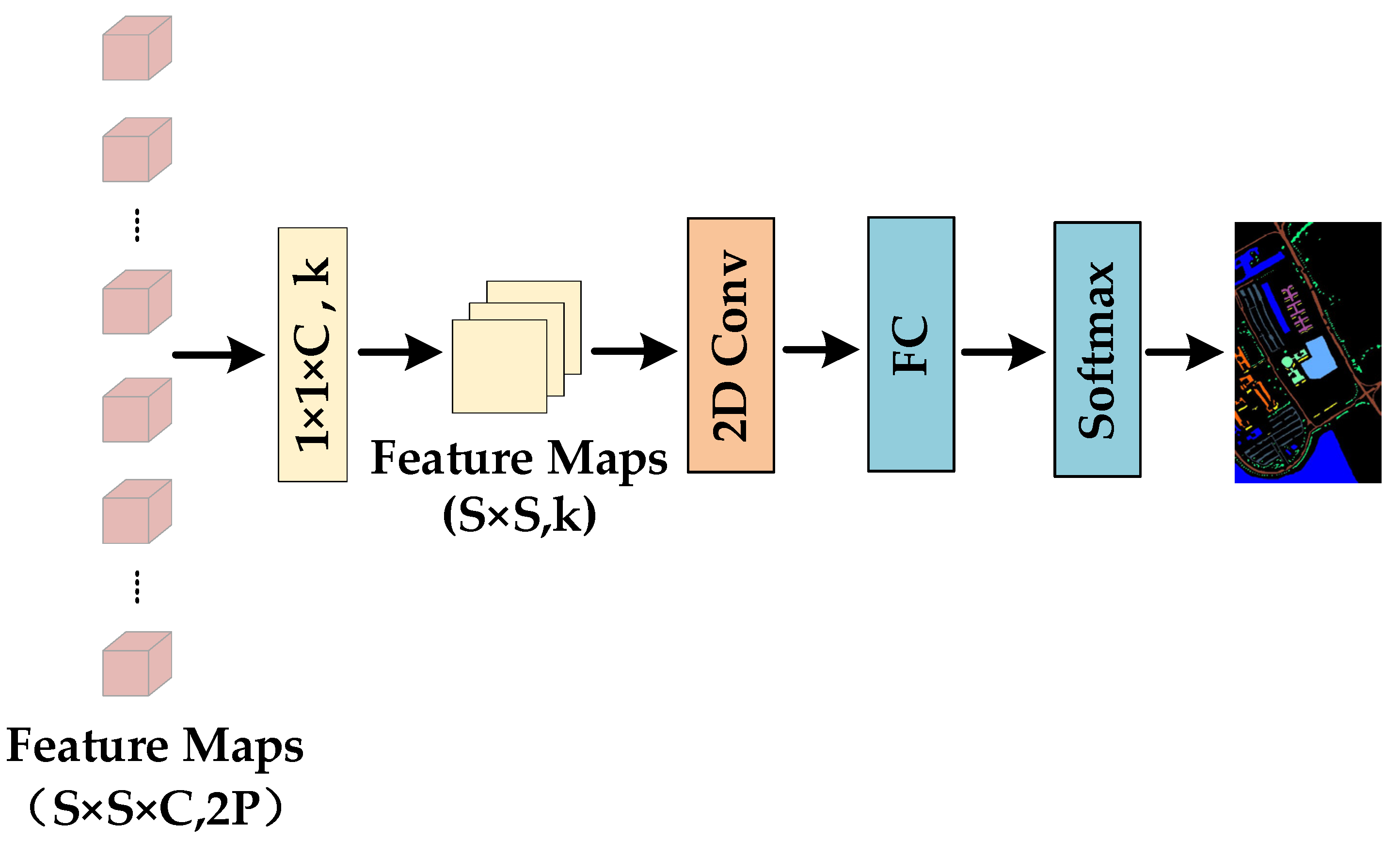
2.3.4. 2DCNN for Classification

As shown in Figure 13, the result of the feature attention module enters the 2DCNN network to further extract the feature and obtains the final classification result. The purpose of introducing the 2DCNN network instead of continuing to use the 3DCNN network is to decrease the sophistication of the network and reduce the parameters in the network. The main steps are the following.
(1) For the result with size { S × S × C , 2 P }, the convolution kernel with size { 1 × 1 × C } is adopted to convert the 3D feature maps with size { S × S × C , 2 P } to the 2D feature maps with size { S × S ,   k }.
(2) Then, the 2D feature maps with size { S × S , k } is sent to the 2D convolutional layers to promote the fusion of features and further extract features with stronger representation ability.
(3) The 2D convolutional layer is concatenated with the fully connected layers. Finally, the SoftMax classifier is employed to predict the category of each pixel.

3. Experimental Result and Analysis

In this chapter, the three HSI datasets utilized in our experiments are described first, and the experimental configurations are, then, presented. Next, the influences of the main parameters for the classification performance of our proposed method TSSFAN are analyzed. Additionally, the proposed TSSFAN is compared to several of the most advanced classification methods to verify the superiorities.

3.1. Data Description

In our experiment, we consider three openly accessible HSI datasets, including Indian Pines (IP), University of Pavia (UP), and Salinas Scene (SA).
(1)
Indian Pines (IP): IP was acquired by a sensor on June 1992, in which the spatial size is 145 × 145 and the number of the spectral band is 224. Specifically, its spectral resolution is 10 nm. Moreover, the range of wavelength in IP is 0.4–2.5 μm. Additionally, sixteen categories are contained in IP, and only 200 effective bands in IP can be utilized because the 24 bands that could carry noise information are excluded.
(2)
University of Pavia (UP): UP is acquired by a sensor known as the ROSIS sensor, in which the spatial size is 610 × 340 and the number of the spectral band is 115. Moreover, the range of wavelength in UP is 0.43–0.86 μm. Specifically, nine categories are contained in UP with 42,776 labeled pixels. In the experiment, only 103 effective bands in UP can be utilized because the 12 bands that could carry noise information are excluded.
(3)
Salinas Scene (SA): SA is acquired by a hyperspectral sensor, in which the spatial size is 512 × 217 and the number of the spectral band is 224. Additionally, sixteen categories are contained in SA, and only 204 effective bands in SA can be utilized because the 20 bands that could carry noise information are excluded.
Figure 14, Figure 15 and Figure 16 present the false-color maps and the ground-truth images of IP, UP, and SA, respectively. In our experiment, 10%, 10%, and 80% of the total samples are randomly chosen as training, validation, and testing for IP while 1%, 1%, and 98% for UP and SA. Table 1, Table 2 and Table 3 present the details.

3.2. Experimental Configuration

All experiments were implemented on the computer including an AMD Ryzen 7 4800H CPU and an Nvidia GeForce RTX2060 GPU. We employed Windows 10 as the operating system, using the PyTorch1.2.0 deep-learning framework and a Python 3.6 compiler. In our experiments, overall accuracy (OA), average accuracy (AA), and Kappa coefficient (Kappa) were adopted as the evaluation metric, which aimed to quantitatively assess the classification performance.

3.3. Analysis of Parameters

In this section, we analyze the influences of the three main parameters for the classification performance of our proposed TSSFAN, including learning rate, spectral dimension, and spatial size.
(1)
Learning rate: During the gradient descent process of a deep-learning model, the weights are constantly updated. A few hyperparameters play an instrumental role in controlling this process properly, and one of them is the learning rate. The convergence capability and the convergence speed of the network can be productively regulated by a suitable learning rate. In our trials, the effect of the learning rate on the classification performance is tested, where the value of the learning rate is set to {0.00005,0.0001,0.0003,0.0005,0.001,0.003,0.005,0.008}. Figure 17 shows the experimental results.
From Figure 17, we can observe that there is a gradual rise in accuracy as the learning rate increases from 0.00005 to 0.001, while there is a considerable drop in learning rate further growing from 0.001 to 0.008 for all three datasets. The convergence speed of the network would be reduced when the learning rate is lower, which extends the learning time of the model and weakens the classification performance. However, the network would fail to converge or converge to the local optimum if the learning rate is too high, which can also negatively affect the classification performance. Based on the experimental result, 0.001 is chosen as the optimal learning rate for the three datasets to acquire the best classification performance.
(2)
Spectral dimension: Input-1 contains more spectral information and less spatial information. The spectral dimension in Input-1 determines how much spectral information is available to classify the pixels. We tested the impact of the spectral dimension in Input-1. In our experiments, the spectral dimension in Input-1 is set to {21,23,25,27,29,31,33} to capture sufficient spectral information. Figure 18 presents the experimental results.
Figure 18 shows that there is a trend of rising first and, then, falling with the spectral dimension increasing from 21 to 33 for the three datasets. At the beginning, the classification accuracy increases because more spectral information could be provided with the spectral dimension increasing. Nevertheless, with the spectral dimension further increasing, although more spectral information could be supplied, some noise information is also introduced to reduce the classification accuracy. Figure 18 reveals that we achieve the highest classification accuracy when we fix the spectral dimension to 27 for IN and SA datasets and 23 for UP datasets. The spectral dimension in this situation can provide sufficient spectral information. Although some noise information is also introduced, it can be effectively suppressed by the spectral attention in the network. To be mentioned, since Input-2 contains less spectral information, we preset the spectral dimension as 9 for the three datasets, which minimizes the computing sophistication while guaranteeing the basic spectral information.
(3)
Spatial size: Input-2 contains more spatial information and less spectral information. The spatial size in Input-2 determines how much spatial information is available to classify the pixels. We test the impact of the spatial size in Input-2. In our experiment, the spatial size is set as {25 × 25, 27 × 27, 29 × 29, 31 × 31, 33 × 33, 35 × 35, 37 × 37}. Figure 19 presents the experimental results.
Figure 19 illustrates that there is a gradual improvement and, then, a gradual fall with the spatial size increasing from 25 to 37 for the three datasets. In the initial stage, the classification accuracy grows because more spatial context and spatial structures could be available with the spatial size increasing. However, with the spatial size further increasing, pixels and spatial structures belonging to different classes will be introduced, which reduces the classification performance. Figure 19 indicates that the highest classification accuracy is obtained when we fix the spatial size as 33 × 33 for the three datasets. To be mentioned, since Input-1 contains less spatial information, we preset the spatial size to 9 × 9 for the three datasets, which ensures the basic spatial information while minimizing the computational complexity.
According to the above parameter analysis, Table 4 lists all final parameters.

3.4. Comparisons to the State-of-the-Art Methods

In our experiment, we compare the presented TSSFAN method with SVM [16], two-dimensional convolutional neural network (2DCNN) [43], three-dimensional convolutional neural network (3DCNN) [54], spectral–spatial residual network (SSRN) [39], hybrid spectral CNN (HybridSN) [64], and spectral–spatial attention network (SSAN) [41].
Table 5, Table 6 and Table 7 show the classification performance of each method for IP, UP, and SA. Compared with other competitor models, our proposed TSSFAN acquires the highest OA, AA, and Kappa for the three datasets. In particular, our proposed TSSFAN can still achieve a pretty good classification accuracy of 98.26% under the condition that there are only 1% training samples for Pavia University. The main reason is that our proposed method creates two inputs with different spectral dimensions and spatial sizes for the network, which can accurately and separately explore the spectral and spatial features even if we only use a very small training set. Although 2DCNN, 3DCNN, SSRN, and HybridSN design different network structures to acquire stronger classification performance, our presented TSSFAN method obtains a higher OA than for all three datasets. In addition, our presented TSSFAN acquires better per-class accuracy than the competitor methods in most cases. Especially, our proposed method achieves 100% accuracy in the Alfalfa and Grass-pasture-mowed categories for Indian Pines and achieves 100% accuracy in the Brocoli_green_weeds_2 and Lettuce_romaine_5wk categories for Salinas. The main reason is that our method designs two-branch 3DCNN with attention modules to focus on more discriminative spectral channels and spatial structures, which can effectively enhance the classification performance. Moreover, although SSAN utilizes the attention mechanism to concentrate on more significant information in the classification task, our proposed TSSFAN method acquires better OA for all three datasets. This is largely because our method constructs the feature attention module, which can automatically adjust the weights of different features based on their contributions for the classification. By the constructed feature attention module, different features are given different weights based on their contributions for the classification task, so the classification accuracy will be improved. As a result, the superiorities of the presented TSSFAN by creating two inputs with different size to, respectively, emphasize accurately extracting spectral information and spatial information, designing two-branch 3DCNN with attention modules to focus on more discriminative spectral channels and spatial structures, and constructing the feature attention module to concentrate on the feature contributing more to the classification tasks are completely verifiable.
Figure 20, Figure 21 and Figure 22 depict the corresponding classification results of each classification method for the three HSI datasets, respectively. As presented in Figure 20, Figure 21 and Figure 22, we find that the classification figures acquired by SSRN, HybridSN, and SSAN have smoother boundaries and edges, while those acquired by SVM, 2DCNN, and 3DCNN present more misclassifications. However, our proposed TSSFAN achieves the more accurate classification map, which presents fewer classification errors and smoother boundaries and edges. The main reason is that TSSFAN introduces the attention mechanism to focus on more discriminative information for classification, which can provide more a detailed and accurate classification map.
Finally, we test the computational efficiency of 2DCNN, 3DCNN, and TSSFAN methods on the three datasets to verify the superiority of the hybrid architecture. From Table 8, we find that the calculation time of the presented TSSFAN, including training and testing time, is much less than that of 3DCNN but larger than that of 2DCNN for all three datasets. This is mainly because our proposed TSSFAN designs the hybrid architecture of 3D–2DCNN, which can not only make the network lightweight but also reduces the complexity of the model remarkably.

4. Conclusions

In this paper, a novel two-branch spectral–spatial-feature attention network (TSSFAN) is proposed for HSI classification. TSSFAN designs two parallel 3DCNN branches with attention modules for two inputs with different spectral dimensions and spatial sizes to, respectively, focus on extracting the more discriminative spectral features and spatial features. Moreover, TSSFAN constructs the feature attention module to automatically adjust the weights of different features based on their contributions for classification to remarkably enhance the classification performance and utilize 2DCNN to obtain the final classification result. To verify the effectiveness and superiorities of the proposed method, TSSFAN is compared with several advanced classification methods on three real HSI datasets. The experimental results confirm that our proposed TSSFAN can fully extract more discriminative spectral and spatial features to further improve the classification accuracy. In addition, TSSFAN achieves the highest classification accuracy and clearly performs better than the other compared methods. Nevertheless, there still exist some points that could be further improved. In our further work, the research will focus on how to optimize a deep-learning framework with an attention mechanism to extract more discriminative spectral–spatial features under the small training samples situation and further improve the classification performance.

Author Contributions

Conceptualization, H.W. and D.L.; methodology, H.W., D.L., Y.W. and X.L.; software, H.W. and D.L.; validation, H.W., F.K. and Q.W.; formal analysis, H.W. and D.L.; H.W. wrote the original draft; D.L. gave constructive suggestions and revised the manuscript. All authors have read and agreed to the published version of the manuscript.

Funding

This research was funded by the National Natural Science Foundation of China (grant no. 61801214) and National Key Laboratory Foundation (contract no. 6142411192112).

Conflicts of Interest

The authors declare no conflict of interest.

References

  1. Tao, C.; Wang, Y.J.; Cui, W.B.; Zou, B.; Zou, Z.R.; Tu, Y.L. A transferable spectroscopic diagnosis model for predicting arsenic contamination in soil. Sci. Total. Environ. 2019, 669, 964–972. [Google Scholar] [CrossRef] [PubMed]
  2. Ghamisi, P.; Plaza, J.; Chen, Y.S.; Li, J.; Plaza, A. Advanced Spectral Classifiers for Hyperspectral Images A review. IEEE Geosci. Remote. Sens. Mag. 2017, 5, 8–32. [Google Scholar] [CrossRef] [Green Version]
  3. Konig, M.; Birnbaum, G.; Oppelt, N. Mapping the Bathymetry of Melt Ponds on Arctic Sea Ice Using Hyperspectral Imagery. Remote Sens. 2020, 12, 2623. [Google Scholar] [CrossRef]
  4. Lu, B.; Dao, P.D.; Liu, J.G.; He, Y.H.; Shang, J.L. Recent Advances of Hyperspectral Imaging Technology and Applications in Agriculture. Remote Sens. 2020, 12, 2659. [Google Scholar] [CrossRef]
  5. Aneece, I.; Thenkabail, P. Accuracies Achieved in Classifying Five Leading World Crop Types and their Growth Stages Using Optimal Earth Observing-1 Hyperion Hyperspectral Narrowbands on Google Earth Engine. Remote Sens. 2018, 10, 2027. [Google Scholar] [CrossRef] [Green Version]
  6. Gao, Q.S.; Lim, S.; Jia, X.P. Hyperspectral Image Classification Using Convolutional Neural Networks and Multiple Feature Learning. Remote Sens. 2018, 10, 299. [Google Scholar] [CrossRef] [Green Version]
  7. Zabalza, J.; Ren, J.C.; Zheng, J.B.; Han, J.W.; Zhao, H.M.; Li, S.T.; Marshall, S. Novel Two-Dimensional Singular Spectrum Analysis for Effective Feature Extraction and Data Classification in Hyperspectral Imaging. IEEE Trans. Geosci. Remote. Sens. 2015, 53, 4418–4433. [Google Scholar] [CrossRef] [Green Version]
  8. Du, B.; Zhao, R.; Zhang, L.P.; Zhang, L.F. A spectral-spatial based local summation anomaly detection method for hyperspectral images. Signal Process. 2016, 124, 115–131. [Google Scholar] [CrossRef]
  9. Zhang, L.F.; Zhang, L.P.; Du, B.; You, J.E.; Tao, D.C. Hyperspectral image unsupervised classification by robust manifold matrix factorization. Inf. Sci. 2019, 485, 154–169. [Google Scholar] [CrossRef]
  10. Li, W.; Wu, G.D.; Zhang, F.; Du, Q.A. Hyperspectral Image Classification Using Deep Pixel-Pair Features. IEEE Trans. Geosci. Remote. Sens. 2017, 55, 844–853. [Google Scholar] [CrossRef]
  11. Bitar, A.W.; Cheong, L.F.; Ovarlez, J.P. Sparse and Low-Rank Matrix Decomposition for Automatic Target Detection in Hyperspectral Imagery. IEEE Trans. Geosci. Remote. Sens. 2019, 57, 5239–5251. [Google Scholar] [CrossRef] [Green Version]
  12. Lu, X.Q.; Zheng, X.T.; Yuan, Y. Remote Sensing Scene Classification by Unsupervised Representation Learning. IEEE Trans. Geosci. Remote. Sens. 2017, 55, 5148–5157. [Google Scholar] [CrossRef]
  13. Masarczyk, W.; Glomb, P.; Grabowski, B.; Ostaszewski, M. Effective Training of Deep Convolutional Neural Networks for Hyperspectral Image Classification through Artificial Labeling. Remote Sens. 2020, 12, 2653. [Google Scholar] [CrossRef]
  14. Blanco, S.R.; Heras, D.B.; Arguello, F. Texture Extraction Techniques for the Classification of Vegetation Species in Hyperspectral Imagery: Bag of Words Approach Based on Superpixels. Remote Sens. 2020, 12, 2633. [Google Scholar] [CrossRef]
  15. Qamar, F.; Dobler, G. Pixel-Wise Classification of High-Resolution Ground-Based Urban Hyperspectral Images with Convolutional Neural Networks. Remote Sens. 2020, 12, 2540. [Google Scholar] [CrossRef]
  16. Melgani, F.; Bruzzone, L. Classification of hyperspectral remote sensing images with support vector machines. IEEE Trans. Geosci. Remote. Sens. 2004, 42, 1778–1790. [Google Scholar] [CrossRef] [Green Version]
  17. Zhang, L.P.; Zhang, L.F.; Du, B. Deep Learning for Remote Sensing Data A technical tutorial on the state of the art. IEEE Geosci. Remote. Sens. Mag. 2016, 4, 22–40. [Google Scholar] [CrossRef]
  18. Liu, Z.; Tang, B.; He, X.F.; Qiu, Q.C.; Liu, F. Class-Specific Random Forest with Cross-Correlation Constraints for Spectral-Spatial Hyperspectral Image Classification. IEEE Geosci. Remote. Sens. Lett. 2017, 14, 257–261. [Google Scholar] [CrossRef]
  19. Bajpai, S.; Singh, H.V.; Kidwai, N.R. Feature Extraction & Classification of Hyperspectral Images using Singular Spectrum Analysis & Multinomial Logistic Regression Classifiers. In Proceedings of the 2017 International Conference on Multimedia, Signal Processing and Communication Technologies (IMPACT), Aligarh, India, 24–26 November 2017; IEEE: Piscataway, NJ, USA, 2017; pp. 97–100. [Google Scholar]
  20. Li, W.; Chen, C.; Su, H.J.; Du, Q. Local Binary Patterns and Extreme Learning Machine for Hyperspectral Imagery Classification. IEEE Trans. Geosci. Remote Sens. 2015, 53, 3681–3693. [Google Scholar] [CrossRef]
  21. Dalla Mura, M.; Villa, A.; Benediktsson, J.A.; Chanussot, J.; Bruzzone, L. Classification of Hyperspectral Images by Using Extended Morphological Attribute Profiles and Independent Component Analysis. IEEE Geosci. Remote Sens. Lett. 2011, 8, 542–546. [Google Scholar] [CrossRef] [Green Version]
  22. Cao, C.H.; Deng, L.; Duan, W.; Xiao, F.; Yang, W.C.; Hu, K. Hyperspectral image classification via compact-dictionary-based sparse representation. Multimed. Tools Appl. 2019, 78, 15011–15031. [Google Scholar] [CrossRef]
  23. Li, D.; Wang, Q.; Kong, F.Q. Adaptive kernel sparse representation based on multiple feature learning for hyperspectral image classification. Neurocomputing 2020, 400, 97–112. [Google Scholar] [CrossRef]
  24. Li, D.; Wang, Q.; Kong, F.Q. Superpixel-feature-based multiple kernel sparse representation for hyperspectral image classification. Signal Process. 2020, 176, 107682. [Google Scholar] [CrossRef]
  25. Yang, W.D.; Peng, J.T.; Sun, W.W.; Du, Q. Log-Euclidean Kernel-Based Joint Sparse Representation for Hyperspectral Image Classification. IEEE J. Sel. Top. Appl. Earth Obs. Remote Sens. 2019, 12, 5023–5034. [Google Scholar] [CrossRef]
  26. Li, S.T.; Song, W.W.; Fang, L.Y.; Chen, Y.S.; Ghamisi, P.; Benediktsson, J.A. Deep Learning for Hyperspectral Image Classification: An Overview. IEEE Trans. Geosci. Remote Sens. 2019, 57, 6690–6709. [Google Scholar] [CrossRef] [Green Version]
  27. Mou, L.C.; Ghamisi, P.; Zhu, X.X. Deep Recurrent Neural Networks for Hyperspectral Image Classification. IEEE Trans. Geosci. Remote Sens. 2017, 55, 3639–3655. [Google Scholar] [CrossRef] [Green Version]
  28. Wu, H.; Prasad, S. Convolutional Recurrent Neural Networks for Hyperspectral Data Classification. Remote Sens. 2017, 9, 298. [Google Scholar] [CrossRef] [Green Version]
  29. Fang, L.Y.; Liu, G.Y.; Li, S.T.; Ghamisi, P.; Benediktsson, J.A. Hyperspectral Image Classification with Squeeze Multibias Network. IEEE Trans. Geosci. Remote Sens. 2019, 57, 1291–1301. [Google Scholar] [CrossRef]
  30. Ding, C.; Li, Y.; Xia, Y.; Wei, W.; Zhang, L.; Zhang, Y.N. Convolutional Neural Networks Based Hyperspectral Image Classification Method with Adaptive Kernels. Remote Sens. 2017, 9, 618. [Google Scholar] [CrossRef] [Green Version]
  31. Chen, Y.S.; Lin, Z.H.; Zhao, X.; Wang, G.; Gu, Y.F. Deep Learning-Based Classification of Hyperspectral Data. IEEE J. Sel. Top. Appl. Earth Obs. Remote Sens. 2014, 7, 2094–2107. [Google Scholar] [CrossRef]
  32. Cheng, G.; Li, Z.P.; Han, J.W.; Yao, X.W.; Guo, L. Exploring Hierarchical Convolutional Features for Hyperspectral Image Classification. IEEE Trans. Geosci. Remote Sens. 2018, 56, 6712–6722. [Google Scholar] [CrossRef]
  33. Li, W.; Chen, C.; Zhang, M.M.; Li, H.C.; Du, Q. Data Augmentation for Hyperspectral Image Classification with Deep CNN. IEEE Geosci. Remote Sens. Lett. 2019, 16, 593–597. [Google Scholar] [CrossRef]
  34. Paoletti, M.E.; Haut, J.M.; Fernandez-Beltran, R.; Plaza, J.; Plaza, A.; Li, J.; Pla, F. Capsule Networks for Hyperspectral Image Classification. IEEE Trans. Geosci. Remote Sens. 2019, 57, 2145–2160. [Google Scholar] [CrossRef]
  35. Song, W.W.; Li, S.T.; Fang, L.Y.; Lu, T. Hyperspectral Image Classification with Deep Feature Fusion Network. IEEE Trans. Geosci. Remote Sens. 2018, 56, 3173–3184. [Google Scholar] [CrossRef]
  36. Chen, Y.S.; Zhao, X.; Jia, X.P. Spectral-Spatial Classification of Hyperspectral Data Based on Deep Belief Network. IEEE J. Sel. Top. Appl. Earth Obs. Remote Sens. 2015, 8, 2381–2392. [Google Scholar] [CrossRef]
  37. Hu, W.; Huang, Y.Y.; Wei, L.; Zhang, F.; Li, H.C. Deep Convolutional Neural Networks for Hyperspectral Image Classification. J. Sens. 2015, 2015. [Google Scholar] [CrossRef] [Green Version]
  38. Chen, Y.S.; Jiang, H.L.; Li, C.Y.; Jia, X.P.; Ghamisi, P. Deep Feature Extraction and Classification of Hyperspectral Images Based on Convolutional Neural Networks. IEEE Trans. Geosci. Remote Sens. 2016, 54, 6232–6251. [Google Scholar] [CrossRef] [Green Version]
  39. Zhong, Z.L.; Li, J.; Luo, Z.M.; Chapman, M. Spectral-Spatial Residual Network for Hyperspectral Image Classification: A 3-D Deep Learning Framework. IEEE Trans. Geosci. Remote Sens. 2018, 56, 847–858. [Google Scholar] [CrossRef]
  40. Sellami, A.; Farah, M.; Farah, I.R.; Solaiman, B. Hyperspectral imagery classification based on semi-supervised 3-D deep neural network and adaptive band selection. Expert Syst. Appl. 2019, 129, 246–259. [Google Scholar] [CrossRef]
  41. Mei, X.G.; Pan, E.T.; Ma, Y.; Dai, X.B.; Huang, J.; Fan, F.; Du, Q.L.; Zheng, H.; Ma, J.Y. Spectral-Spatial Attention Networks for Hyperspectral Image Classification. Remote Sens. 2019, 11, 963. [Google Scholar] [CrossRef] [Green Version]
  42. Liu, B.; Zhang, Y.; He, D.J.; Li, Y.X. Identification of Apple Leaf Diseases Based on Deep Convolutional Neural Networks. Symmetry 2018, 10, 11. [Google Scholar] [CrossRef] [Green Version]
  43. Makantasis, K.; Karantzalos, K.; Doulamis, A.; Doulamis, N. Deep supervised learning for hyperspectral data classification through convolutional neural networks. In Proceedings of the 2015 IEEE International Symposium on Geoscience and Remote Sensing Symposium (IGARSS), Milan, Italy, 26–31 July 2015; IEEE: Piscataway, NJ, USA, 2015; pp. 4959–4962. [Google Scholar]
  44. Gu, J.X.; Wang, Z.H.; Kuen, J.; Ma, L.Y.; Shahroudy, A.; Shuai, B.; Liu, T.; Wang, X.X.; Wang, G.; Cai, J.F.; et al. Recent advances in convolutional neural networks. Pattern Recognit. 2018, 77, 354–377. [Google Scholar] [CrossRef] [Green Version]
  45. Sun, Y.A.; Xue, B.; Zhang, M.J.; Yen, G.G. Evolving Deep Convolutional Neural Networks for Image Classification. IEEE Trans. Evol. Comput. 2020, 24, 394–407. [Google Scholar] [CrossRef] [Green Version]
  46. Li, Y.S.; Zhang, Y.J.; Huang, X.; Ma, J.Y. Learning Source-Invariant Deep Hashing Convolutional Neural Networks for Cross-Source Remote Sensing Image Retrieval. IEEE Trans. Geosci. Remote Sens. 2018, 56, 6521–6536. [Google Scholar] [CrossRef]
  47. Ma, J.Y.; Yu, W.; Liang, P.W.; Li, C.; Jiang, J.J. FusionGAN: A generative adversarial network for infrared and visible image fusion. Inf. Fusion 2019, 48, 11–26. [Google Scholar] [CrossRef]
  48. Paoletti, M.E.; Haut, J.M.; Fernandez-Beltran, R.; Plaza, J.; Plaza, A.J.; Pla, F. Deep Pyramidal Residual Networks for Spectral-Spatial Hyperspectral Image Classification. IEEE Trans. Geosci. Remote Sens. 2019, 57, 740–754. [Google Scholar] [CrossRef]
  49. Tian, T.; Li, C.; Xu, J.K.; Ma, J.Y. Urban Area Detection in Very High Resolution Remote Sensing Images Using Deep Convolutional Neural Networks. Sensors 2018, 18, 904. [Google Scholar] [CrossRef] [Green Version]
  50. Wang, Z.Y.; Yi, P.; Jiang, K.; Jiang, J.J.; Han, Z.; Lu, T.; Ma, J.Y. Multi-Memory Convolutional Neural Network for Video Super-Resolution. IEEE Trans. Image Process. 2019, 28, 2530–2544. [Google Scholar] [CrossRef] [PubMed]
  51. Karim, F.; Majumdar, S.; Darabi, H.; Chen, S. LSTM Fully Convolutional Networks for Time Series Classification. IEEE Access 2018, 6, 1662–1669. [Google Scholar] [CrossRef]
  52. Xu, Y.; Bao, Y.Q.; Chen, J.H.; Zuo, W.M.; Li, H. Surface fatigue crack identification in steel box girder of bridges by a deep fusion convolutional neural network based on consumer-grade camera images. Struct. Health Monit. Int. J. 2019, 18, 653–674. [Google Scholar] [CrossRef]
  53. Ma, X.L.; Dai, Z.; He, Z.B.; Ma, J.H.; Wang, Y.; Wang, Y.P. Learning Traffic as Images: A Deep Convolutional Neural Network for Large-Scale Transportation Network Speed Prediction. Sensors 2017, 17, 818. [Google Scholar] [CrossRef] [PubMed] [Green Version]
  54. Ben Hamida, A.; Benoit, A.; Lambert, P.; Ben Amar, C. 3-D Deep Learning Approach for Remote Sensing Image Classification. IEEE Trans. Geosci. Remote Sens. 2018, 56, 4420–4434. [Google Scholar] [CrossRef] [Green Version]
  55. Jingmei, L.; Zhenxin, X.; Jianli, L.; Jiaxiang, W. An Improved Human Action Recognition Method Based on 3D Convolutional Neural Network. In Advanced Hybrid Information Processing. ADHIP 2018. Lecture Notes of the Institute for Computer Sciences, Social Informatics and Telecommunications Engineering; Liu, S., Yang, G., Eds.; Springer: Cham, Switzerland, 2019; Volume 279, pp. 37–46. [Google Scholar] [CrossRef]
  56. Liu, X.; Yang, X.D. Multi-stream with Deep Convolutional Neural Networks for Human Action Recognition in Videos. In Neural Information Processing. ICONIP 2018. Lecture Notes in Computer Science; Cheng, L., Leung, A.C.S., Ozawa, S., Eds.; Springer: Cham, Switzerland, 2018; Volume 11301, pp. 251–262. [Google Scholar]
  57. Saveliev, A.; Uzdiaev, M.; Dmitrii, M. Aggressive action recognition using 3D CNN architectures. In Proceedings of the 12th International Conference on Developments in eSystems Engineering 2019, Kazan, Russia, 7–10 October 2019; AlJumeily, D., Hind, J., Mustafina, J., AlHajj, A., Hussain, A., Magid, E., Tawfik, H., Eds.; IEEE: Piscataway, NJ, USA, 2019; pp. 890–895. [Google Scholar]
  58. Zhang, J.H.; Chen, L.; Tian, J. 3D Convolutional Neural Network for Action Recognition. In Computer Vision, Pt I; Yang, J., Hu, Q., Cheng, M.M., Wang, L., Liu, Q., Bai, X., Meng, D., Eds.; Springer: Singapore, 2017; Volume 771, pp. 600–607. [Google Scholar]
  59. Feng, S.Y.; Chen, T.Y.; Sun, H. Long Short-Term Memory Spatial Transformer Network. In Proceedings of the 2019 IEEE 8th Joint International Information Technology and Artificial Intelligence Conference (ITAIC), Chongqing, China, 24–26 May 2019; IEEE: Piscataway, NJ, USA, 2019; pp. 239–242. [Google Scholar]
  60. Liang, L.; Cao, J.D.; Li, X.Y.; You, A.N. Improvement of Residual Attention Network for Image Classification. In Intelligence Science and Big Data Engineering. Visual Data Engineering. IScIDE 2019. Lecture Notes in Computer Science; Cui, Z., Pan, J., Zhang, S., Xiao, L., Yang, J., Eds.; Springer: Cham, Switzerland; New York, NY, USA, 2019; Volume 11935, pp. 529–539. [Google Scholar]
  61. Ling, H.F.; Wu, J.Y.; Huang, J.R.; Chen, J.Z.; Li, P. Attention-based convolutional neural network for deep face recognition. Multimed. Tools Appl. 2020, 79, 5595–5616. [Google Scholar] [CrossRef]
  62. Woo, S.H.; Park, J.; Lee, J.Y.; Kweon, I.S. CBAM: Convolutional Block Attention Module. In Computer Vision-ECCV 2018, Part VII, Proceedings of the 15th European Conference on Computer Vision (ECCV), Munich, Germany, 8–14 September 2018; Ferrari, V., Hebert, M., Sminchisescu, C., Weiss, Y., Eds.; Springer International Publishing: New York, NY, USA, 2018; Volume 11211, pp. 3–19. [Google Scholar]
  63. Zhong, X.; Gong, O.B.; Huang, W.X.; Li, L.; Xia, H.X. Squeeze-and-excitation wide residual networks in image classification. In Proceedings of the 2019 IEEE International Conference on Image Processing, Taipei, Taiwan, 22–25 September 2019; IEEE: Piscataway, NJ, USA, 2019; pp. 395–399. [Google Scholar]
  64. Roy, S.K.; Krishna, G.; Dubey, S.R.; Chaudhuri, B.B. HybridSN: Exploring 3-D-2-D CNN Feature Hierarchy for Hyperspectral Image Classification. IEEE Geosci. Remote Sens. Lett. 2020, 17, 277–281. [Google Scholar] [CrossRef] [Green Version]
Figure 1. Illustration of typical 2DCNN structure.
Remotesensing 13 04262 g001
Figure 2. Illustration of typical 3DCNN structure.
Remotesensing 13 04262 g002
Figure 3. Illustration of a typical attention module.
Remotesensing 13 04262 g003
Figure 4. Flowchart of our proposed model.
Remotesensing 13 04262 g004
Figure 5. Construction of two inputs with different spectral dimensions and spatial sizes.
Remotesensing 13 04262 g005
Figure 6. 3DCNN with spectral–spatial attention.
Remotesensing 13 04262 g006
Figure 7. Spectral–spatial attention module.
Remotesensing 13 04262 g007
Figure 8. Attention maps: (a) spectral attention map; (b) spatial attention map.
Remotesensing 13 04262 g008
Figure 9. 3DCNN with spatial–spectral attention.
Remotesensing 13 04262 g009
Figure 10. Spatial–spectral attention module.
Remotesensing 13 04262 g010
Figure 11. Co-training model.
Remotesensing 13 04262 g011
Figure 12. Feature attention module.
Remotesensing 13 04262 g012
Figure 13. 2DCNN for classification.
Remotesensing 13 04262 g013
Figure 14. Indian Pines: (a) false-color map; (b) ground-truth image.
Remotesensing 13 04262 g014
Figure 15. University of Pavia: (a) false-color map; (b) ground-truth image.
Remotesensing 13 04262 g015
Figure 16. Salinas Scene: (a) false-color map; (b) ground-truth image.
Remotesensing 13 04262 g016
Figure 17. The classification result (OA) of our presented TSSFAN with different learning rates for all three HSI datasets.
Remotesensing 13 04262 g017
Figure 18. The classification result (OA) of our presented TSSFAN with different quantities of spectral dimensions in Input- 1 for all three HSI datasets.
Remotesensing 13 04262 g018
Figure 19. The classification result (OA) of our presented TSSFAN with different spatial size in Input- 2 for all three HSI datasets.
Remotesensing 13 04262 g019
Figure 20. Classification maps acquired by each method for the Indian Pines dataset: (a) ground-truth image, (b) SVM, (c) 2DCNN, (d) 3DNN, (e) SSRN, (f) HybridSN, (g) SSAN, (h) proposed TSSFAN.
Remotesensing 13 04262 g020
Figure 21. Classification maps acquired by each method for the University of Pavia dataset: (a) ground-truth map, (b) SVM, (c) 2DCNN, (d) 3DNN, (e) SSRN, (f) HybridSN, (g) SSAN, (h) proposed TSSFAN.
Remotesensing 13 04262 g021
Figure 22. Classification maps acquired by each method for the Salinas Scene dataset: (a) ground-truth map, (b) SVM, (c) 2DCNN, (d) 3DNN, (e) SSRN, (f) HybridSN, (g) SSAN, (h) proposed TSSFAN.
Remotesensing 13 04262 g022
Table 1. Number of training, validation, and testing samples for the IP dataset.
ClassNameTrainingValidationTestTotal Samples
1Alfalfa553646
2Corn-notill14314311421428
3Corn-mintill8383664830
4Corn2424189237
5Grass-pasture4848387483
6Grass-trees7373584730
7Grass-pasture-mowed332228
8Hay-windrowed4848382478
9Oats221620
10Soybean-notill9797778972
11Soybean-mintill24624619632455
12Soybean-clean5959475593
13Wheat2121163205
14Woods12712710111265
15Buildings-Grass-Trees-Drives3939308386
16Stone-Steel-Towers997593
Total 10271027819510,249
Table 2. Number of training, validation, and testing samples for the UP dataset.
ClassNameTrainingValidationTestTotal Samples
1Asphalt666664996631
2Meadows18618618,27718,649
3Gravel212120572099
4Trees313130023064
5Painted metal sheets131313191345
6Bare Soil505049295029
7Bitumen131313041330
8Self-Blocking Bricks373736083682
9Shadows99929947
Total 42642641,92442,776
Table 3. Number of training, validation, and testing samples for the SA dataset.
ClassNameTrainingValidationTestTotal Samples
1Brocoli_green_weeds_1202019692009
2Brocoli_green_weeds_2373736523726
3Fallow202019361976
4Fallow_rough_plow141413661394
5Fallow_smooth272726242678
6Stubble404038793959
7Celery363635073579
8Grapes_untrained11311311,04511,271
9Soil_vinyard_develop626260796203
10Corn_senesced_green_weeds333332123278
11Lettuce_romaine_4wk111110461068
12Lettuce_romaine_5wk191918891927
13Lettuce_romaine_6wk99898916
14Lettuce_romaine_7wk111110481070
15Vinyard_untrained737371227268
16Vinyard_vertical_trellis181817711807
Total 54354353,04354,129
Table 4. All parameters for the three HSI datasets.
DataLearning RateSpectral Dimension (Input_1)Spatial Size (Input_1)Spectral Dimension (Input_2)Spatial Size (Input_2)
IP0.001279933
UP0.001239933
SA0.001279933
Table 5. Classification results of each method in Indian Pines (The bold format represents the best result).
ClassSVM2DCNN3DCNNSSRNHybridSNSSANTSSFAN
10.0081.7199.9298.7095.1292.68100.00
227.6293.6995.1095.8395.9595.1896.45
39.7797.8699.0699.8797.9999.3399.67
47.0494.1398.1296.9497.1898.7697.03
563.7998.5097.7097.81100.0099.9599.00
694.0698.3298.1798.7098.9398.4899.29
70.0094.0796.0099.9696.0198.00100.00
899.3099.5399.53100.0099.3099.1099.85
90.0061.1183.3388.8877.7894.4489.81
1025.8097.4398.0698.9798.1798.5198.80
1191.3598.2699.5099.2598.9699.0199.24
1250.4694.9494.7695.6098.1397.3895.47
1369.5696.4998.3899.7397.8499.4699.55
1495.2198.9099.1299.9099.7499.9199.81
1547.5597.6997.1297.5599.1499.4299.61
1688.0991.6795.2496.4378.5795.2497.22
OA62.16
(0.58)
97.1
(0.41)
97.99
(0.22)
98.44
(0.28)
98.19
(0.15)
98.49
(0.13)
98.64
(0.13)
AA48.03
(0.67)
93.38
(0.21)
96.82
(0.30)
97.76
(0.37)
95.55
(0.24)
97.81
(0.25)
98.18
(0.31)
Kappa55.37
(0.39)
96.69
(0.35)
97.71
(0.11)
98.22
(0.30)
95.55
(0.18)
98.28
(0.19)
98.47
(0.17)
Table 6. Classification results of each method in University of Pavia (The bold format represents the best result).
ClassSVM2DCNN3DCNNSSRNHybridSNSSANTSSFAN
189.4784.5094.7696.8995.0395.5297.40
294.1398.9599.4699.9499.7799.9899.91
322.9059.3195.3394.0890.4292.6095.82
482.3670.9481.4090.6687.8395.1592.41
599.2495.2799.2599.6797.3099.2799.94
634.2792.4995.8297.0099.9299.9599.75
70.0875.0689.3782.7199.3297.8798.47
877.9469.4682.5294.6396.8489.7895.25
940.1941.0869.8095.9774.0799.4797.55
OA76.68
(0.47)
87.32
(0.17)
94.37
(0.22)
97.07
(0.23)
96.83
(0.12)
97.56
(0.19)
98.26
(0.14)
AA60.07
(0.40)
76.34
(0.21)
89.74
(0.19)
94.61
(0.20)
93.39
(0.26)
96.62
(0.27)
97.38
(0.28)
Kappa67.89
(0.28)
83.01
(0.15)
92.52
(0.14)
94.61
(0.30)
95.78
(0.16)
96.76
(0.21)
97.70
(0.23)
Table 7. Classification results of each method in Salinas Scene (The bold format represents the best result).
ClassSVM2DCNN3DCNNSSRNHybridSNSSANTSSFAN
197.3395.8598.9992.8899.3999.4599.41
297.7096.8899.8199.2799.90100.00100.00
377.2491.0097.0399.8499.5999.9599.97
457.9783.9894.6496.9395.3899.9999.96
598.9089.6899.5597.6898.3299.7098.37
699.2097.2399.7799.4999.6699.9599.97
799.5498.6898.9099.4699.8199.9499.87
870.0997.8995.8698.5099.4596.9897.24
999.6798.62100.0099.9599.8999.9999.99
1089.3096.3397.3297.6598.9198.6499.56
1189.6887.2294.3297.6998.0499.6299.30
1293.7190.8579.1991.6895.0799.58100.00
1363.8379.6593.3897.6187.1096.6998.66
1496.7891.8897.1796.9898.1799.1598.41
1575.2090.4199.7898.6297.4497.2398.65
1697.6597.3796.2599.1299.7295.9298.82
OA86.27
(0.64)
94.81
(0.21)
97.39
(0.11)
98.29
(0.29)
98.70
(0.16)
98.64
(0.23)
99.02
(0.12)
AA87.74
(0.42)
92.71
(0.37)
96.37
(0.41)
97.70
(0.23)
97.86
(0.33)
98.92
(0.28)
99.25
(0.05)
Kappa84.73
(0.51)
94.21
(0.18)
97.09
(0.23)
98.1
(0.26)
98.55
(0.20)
98.48
(0.31)
98.87
(0.16)
Table 8. Computational efficiency of 2DCNN, 3DCNN, and TSSFAN on the three HSI datasets.
Data2DCNN3DCNNTSSFAN
Training(s)Testing(s)Training(s)Testing(s)Training(s)Testing(s)
IP72.11.4306.03.8204.32.5
UP45.42.2177.611.4110.34.3
SA48.52.7192.114.5125.45.0
Publisher’s Note: MDPI stays neutral with regard to jurisdictional claims in published maps and institutional affiliations.

