Article

A Universal Fuzzy Logic Optical Water Type Scheme for the Global Oceans

1
State Key Laboratory of Urban and Regional Ecology, Research Center for Eco-Environmental Sciences, Chinese Academy of Sciences, Beijing 100085, China
2
University of Chinese Academy of Sciences, Beijing 100049, China
*
Author to whom correspondence should be addressed.
Remote Sens. 2021, 13(19), 4018; https://doi.org/10.3390/rs13194018
Submission received: 20 August 2021 / Revised: 5 October 2021 / Accepted: 7 October 2021 / Published: 8 October 2021
(This article belongs to the Special Issue Remote Sensing Applications in Ocean Observation)

Abstract

:
The classification of natural waters is a way to generalize and systematize ocean color science. However, there is no consensus on an optimal water classification template in many contexts. In this study, we conducted an unsupervised classification of the PACE (Plankton, Aerosols, Cloud, and Ocean Ecosystem) synthetic hyperspectral data set, divided the global ocean waters into 15 classes, then obtained a set of fuzzy logic optical water type schemes (abbreviated as the U-OWT in this study) that were tailored for several multispectral satellite sensors, including SeaWiFS, MERIS, MODIS, OLI, VIIRS, MSI, and OLCI. The consistency analysis showed that the performance of U-OWT on different satellite sensors was comparable, and the sensitivity analysis demonstrated the U-OWT could resist a certain degree of input disturbance on remote sensing reflectance. Compared to existing ocean-aimed optical water type schemes, the U-OWT can distinguish more mesotrophic and eutrophic water classes. Furthermore, the U-OWT was highly compatible with other water classification taxonomies, including the trophic state index, the multivariate absorption combinations, and the Forel-Ule Scale, which indirectly demonstrated the potential for global applicability of the U-OWT. This finding was also helpful for the further conversion and unification of different water type taxonomies. As the fundamental basis, the U-OWT can be applied to many oceanic fields that need to be explored in the future. To promote the reproducibility of this study, an IDL®-based standalone U-OWT calculation tool is freely distributed.

Graphical Abstract

1. Introduction

Since the first ocean color-aimed spaceborne instrument, the Coastal Zone Color Scanner Experiment (CZCS), was launched in 1978, together with subsequent ocean color satellite programs SeaWiFS, MODIS, MERIS, VIIRS, OLCI, etc., the synoptic and accurate measurement of ocean ecosystems on a global scale has become a reality [1]. Ocean color remote sensing has been widely applied to and revolutionized many fields of oceanography, such as oceanic modeling, ocean physics, biogeochemical cycles, fisheries, water quality, and natural and man-made hazards [2,3]. The classification of natural waters using different water type taxonomies is a way to generalize and systematize the science of ocean color [3]. Because of the desire to move toward water classification based directly on satellite data [4], some water classification schemes have relied on the apparent optical properties (AOPs), namely reflectances (various ratios of upwelling to downwelling intensity) and diffuse attenuation functions [5]. Jerlov introduced an ocean water classification based on spectral optical attenuation depth (the inverse of the diffuse attenuation coefficient), and he divided the observations into five open oceanic and nine coastal water types [6,7], which laid the foundation for the AOP-based optical water type (OWT) classification. Moore et al. proposed a fuzzy logic-based OWT scheme that was used for blending class-specific Chlorophyll (Chl) inverse algorithms by the membership weight [8]. Over the past 20 years, much effort has been devoted to AOP-based OWT schemes, which have been developed based on huge spectral reflectance datasets from in situ measurements or satellite data (see Section 2.3.1 for more details) [9,10,11,12,13,14,15,16,17,18,19,20,21,22,23,24,25,26,27,28,29,30].
Although the existing AOP-based OWT schemes were effective and elegant in their respective contexts, from the authors’ point of view, there is still the possibility of making some improvements based on the following aspects. First, some existing AOP-based OWT schemes that were developed from in situ or satellite data may include uncertainties. Specifically, in situ data may contain uncertainties caused by experimental and environmental factors, such as calibration, dark signal, data processing, deployment strategies, and sea and sky states. The uncertainties of satellite data can be introduced by a variety of factors, such as pre-launch characterization of the sensor, atmospheric and bi-directional corrections, geo-location, and contamination by adjacent pixels [31]. Furthermore, the spatial mismatches arise when matching up in situ data and satellite data: horizontally, in situ data often cover an area of 1−10 m while ocean color satellite pixels are often more than 100 m; vertically, in situ measurements are usually conducted on discrete depths while satellite measurements represent a water column weighted average [31]. Thus, there are some potential uncertainties when the in situ data-based OWT schemes are applied to satellite data. Second, the spatial and temporal distributions of the in situ or the pixel spectra affect the representativeness of water classifications [30,32]. For instance, the in situ data were mostly collected in the Northern Hemisphere, with few data points representing very oligotrophic gyre areas [33]. On the contrary, when developing OWT schemes based on satellite data, the pixels corresponding to oligotrophic waters cover a large proportion of the overall spectrum. As a result, the satellite data-based-OWT schemes performed better in open oceans, while the in situ data-based OWT schemes often worked better in coastal waters [19]. Third, with the development of hyperspectral remote sensing technology, some of the existing OWT schemes that initially were developed within limited multispectral bands may not encompass all characteristic bands reflecting the bio-optical features of water. Fourth, the existing OWT schemes were mostly designed for one specific ocean color instrument, such as SeaWiFS [11,13,14,17,22], MODIS [10,15], MERIS [15,16,19,20,30], or OLCI [18]; thus it is difficult to migrate these OWT schemes to other satellite sensors. Therefore, it is necessary to develop an OWT scheme that is measurement error-free, suitable for the global ocean waters, and multi-satellite sensors.
In addition to the AOP-based OWT schemes, there are other water classification taxonomies that are suitable for quantitative water quality evaluation, such as the trophic state index (TSI) [34], the absorption coefficient ternary diagram [4,5,34], and the Forel-Ule Scale [23,35,36,37]. Further introduction to these water classification taxonomies is in Section 2.4. Although the abovementioned water classification taxonomies are commonly used, to the best of our knowledge, scant effort has been applied to exploring the relationships and correspondences between the AOP-based OWT schemes and other water type taxonomies which will hinder their comparison and unification in many cases.
Against the above background, the aims of this study were to: (1) develop a fuzzy logic AOP-based OWT scheme (abbreviated as the U-OWT hereafter) for global oceans and multi-satellite sensors; (2) test the robustness and reliability of the U-OWT; (3) explore the relationships between the U-OWT and other water classification taxonomies; (4) apply the U-OWT to the global oceans preliminarily.

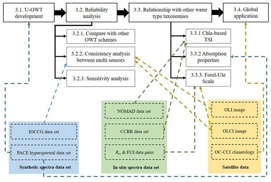
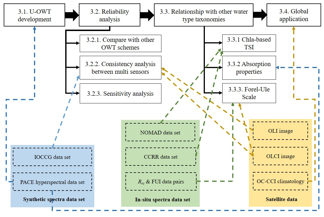
2. Materials and Methods

2.1. Materials

2.1.1. Synthetic Data

The Hydrolight simulated hyperspectral data set (350−800 nm, 5 nm resolution) that was created by the first NASA PACE (Plankton, Aerosol, Cloud, and Ocean Ecosystem) Science Team (NNH13ZDA001N-PACEST) was downloaded from PANGAEA [38]. This data set contains 714 measurement error-free hyperspectral synthetic sea surface remote sensing reflectance Rrs(λ) (sr−1), total absorption atot(λ) (m−1), phytoplankton absorption aph(λ) (m−1), CDOM absorption ag(λ) (m−1), and detrital absorption ad(λ) (m−1) with a solar zenith angle of 30°. The Hydrolight model run was constrained with a set of in situ aph(λ)) spectra collected from NASA’s SeaBASS repository, using the principles outlined in IOCCG Report No. 5 [31]. Because the above in situ aph(λ) spectra were selected from more than 4000 SeaBASS spectra, and together with the random combination of optically active constituents, this synthetic data set was expected to cover all possible natural ocean water IOP-AOP scenarios [30,39], theoretically without duplicate data. This data set was used for the U-OWT scheme development and the IOPs analysis of each U-OWT class.
The Hydrolight synthesized Rrs(λ) and Chla data set with the sun zenith angle of 30° from IOCCG Report No. 5 [31] was used for exploring the robustness and the water quality properties of the U-OWT. The data set contains 500 Rrs(λ) and IOPs spectra pairs for testing and comparing ocean color algorithms. It covers a wide range of natural waters with discrete Chla concentrations from 0.03 to 30 mg/m3. The data set was used for the consistency analysis of the U-OWT among different multispectral satellite sensors, and the water quality parameter analysis of each U-OWT class.

2.1.2. In Situ Data

The NOMAD (NASA bio-Optical Marine Algorithm Data set) version 2 data set is a publicly available, global, high quality in situ bio-optical data set for use in ocean color algorithm development and satellite data product validation activities [40]. The data set includes surface water-leaving radiance Lw, surface downward irradiance Es, and Chla concentration data. After the data filtering, 1052 qualified SeaWiFS-band Rrs(λ) (Rrs = Lw/Es) and Chla data pairs were retrieved from the NOMAD data set.
The CCRR (Coast Colour Round Robin) in situ data set was collected to test algorithms and to assess their accuracy for retrieving water quality parameters [41]. A total number of 336 MERIS level 2 Rrs(λ) and Chla match-ups were extracted from this data set. The Rrs(λ) and Chla data pairs from the NOMAD and the CCRR data sets were used for exploring the water quality properties of each U-OWT class.
Two data sets containing in situ Rrs(λ) and FUI data pairs were used for exploring the relationship between the U-OWT and the Forel-Ule Scale [39]: the first data set was collected from 612 sites covering coastal and oceanic waters around the world [42], the second data set was collected from 195 sites in coastal and oceanic waters off China [43]. Specifically, the hyperspectral Rrs(λ) spectra of these data sets were interpolated to OLCI bands to calculate their dominant OWT (the water class with maximum membership) of the U-OWT.

2.1.3. Satellite Images

Two Landsat-8 OLI and Sentinel-3A OLCI images overpassing Pearl River Estuary on 23 October 2017 were downloaded from the USGS EarthExplore and the EUMETSAT Earth Observation Portal, respectively. The scene center times of the OLI image and the OLCI image were UTC 2:53 and UTC 2:34, respectively; thus, the two images can be regarded as approximately concurrent. The water in Pearl River Estuary is highly turbid and optically complicated [44]; thus, this area was suitable for testing the performance of the U-OWT.
The ESA OC-CCI climatology monthly composite Rrs data set (version 4.2) [45], with 4 km nominal spatial resolution at the equator, was downloaded from the ESA OC-CCI ftp server. As a level 3 binning product, the OC-CCI was composited from multiple sensors (SeaWiFS, MODIS, MERIS, and VIIRS) to SeaWiFS Rrs bands and values. The data set was used to study the global seasonal variability of the relative U-OWT indicators from 1998 to 2019 [46].

2.1.4. Other Data

The relative spectral response functions RSR(λ) of several multispectral satellite sensors were obtained to convolute the hyperspectral Rrs(λ) to the multispectral Rrs(λ). Specifically, the RSR(λ) of SeaWiFS, MERIS, MODIS-Aqua, MODIS-Terra, OLI, VIIRS-NPP, OLCI-S3A, and OLCI-S3B were downloaded from the NASA Ocean Biology Processing Group. The RSR(λ) of MSI-S2A and MSI-S2B were downloaded from the ESA Sentinel website (see Data Availability Statement for more information).

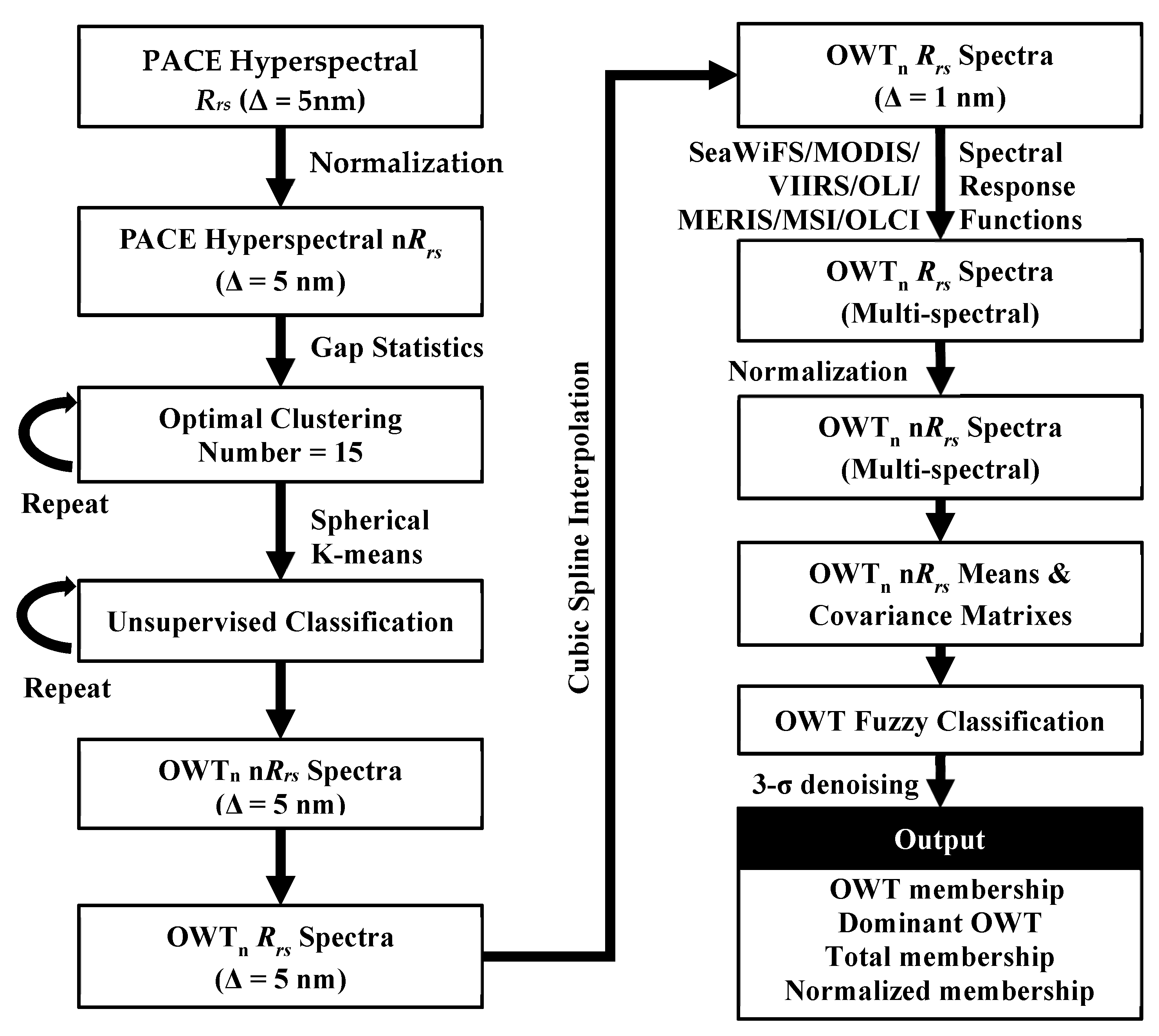
2.2. Development of the U-OWT

(1) The 714 PACE synthetic Rrs spectra were normalized by their Root-Sum-Squares (RSS) [15]:
n R r s ( λ ) = R r s ( λ ) 1 i R r s ( λ i ) 2
where nRrs(λ) is normalized remote sensing reflectance, index i represents the total number of wavelengths, ranging from 1 to 91, and λ represents the wavelength varying from 350 to 800 nm, with 5 nm intervals. The Rrs(λ) spectral shape characteristics are highlighted after the normalized transformation and are more related to the absorption than to the backscattering [11,14].
(2) The optimal clustering number of nRrs(λ) was estimated using the gap statistic method [47]. This step was accomplished using the “clusGap” function in the R® platform. Repeated experiments with the gap method determined that the optimal clustering number was 15.
(3) The spherical k-means clustering (skmeans) method [48] was used to cluster 714 nRrs(λ) spectra into 15 groups. The skmeans is an unsupervised clustering method that employs cosine dissimilarity:
d ( x , p ) = 1 cos ( x , p ) = 1 x , p | x | | p |
where d(x, p) is the cosine dissimilarity between the feature vectors x (here, the nRrs spectra) and centroids p (here, the nRrs mean of each group). The skmeans partitions data into a given number k of groups via minimizing d(x, p) over all samples x to cluster centroids p. Compared to the ordinary k-means method, the skmeans is more suitable for clustering nRrs(λ) spectra, because the cosine dissimilarity places emphasis more on the spectral shape rather than on the spectral amplitude. In addition, the skmeans method was ran 10 times to reduce the effects of random initialization of unsupervised clustering [48]. Finally, the 714 nRrs(λ) spectra (and their original Rrs(λ) spectra) fell into 15 groups (OWT1–OWT15) according to their most frequent clustering results. This step was accomplished using the R® package “skmeans”.
(4) After the unsupervised clustering of each Rrs(λ)/nRrs(λ) spectrum that had a 5 nm interval, the cubic spline interpolation was used to create the hyperspectral Rrs(λ) with 1 nm increments (350−800 nm, 451 bands).
(5) In order to obtain the different multispectral satellite sensors’ Rrs(λ) spectra for each OWT group, spectral bandpass integration was performed on each hyperspectral Rrs spectrum:
R r s - m u l t i ( λ ) = λ 1 λ 2 R r s - h y p e r R S R ( λ ) d λ λ 1 λ 2 R S R ( λ ) d λ
where Rrs-multi(λ) is the band-averaged multispectral remote sensing reflectance, Rrs-hyper is the hyperspectral remote sensing reflectance spectrum. RSR(λ) represents the relative spectral response function of the multispectral satellite sensor. λ is the specific multispectral wavelength between 400−800 nm, i.e., the visible to near-infrared wavelength. λ1 and λ2 are the lower (400 nm) and upper (800 nm) limits of integration, respectively. In this paper, several commonly used multispectral satellite sensors, including SeaWiFS-SEASTAR, MODIS-Aqua, MODIS-Terra, VIIRS-NPP, OLI-Landsat 8, MERIS-ENVISAT, MSI-Sentinel 2A, MSI-Sentinel 2B, OLCI- Sentinel 3A, and OLCI- Sentinel 3B, were selected to develop their corresponding U-OWT schemes.
(6) For each multispectral sensor, the Rrs-multi(λ) spectra of each OWT group were normalized to determine the nRrs-multi(λ) spectra.
(7) Finally, the nRrs-multi(λ) mean and covariance of each OWT were calculated, which are two key statistics for the OWT membership function calculation [13]. Then, the squared Mahalanobis distances of each OWT were acquired [8]:
Z i 2 = ( n R r s M i ) t C o v i 1 ( n R r s M i )
where Z i 2 is the squared Mahalanobis distance, nRrs is the multispectral normalized remote sensing reflectance of a target spectrum or a target pixel, Mi is the nRrs mean of the ith OWT, t represents the transpose of the vector (nRrsMi), and C o v i 1 is the inverse covariance matrix of the ith OWT. In this study, a common weighted covariance matrix was used for the membership calculation of all 15 OWT classes [8].
Then, the membership function was obtained:
f i = 1 F n ( Z i 2 )
where fi is the members belonging to the ith OWT, F n ( Z i 2 ) is the cumulative Chi-square distribution function with n degrees of freedom. Here, for each satellite sensor, n equals their multispectral band numbers. After the membership calculation, three other OWT indicators were also obtained: first, the dominant OWT was defined as the OWT of maximum membership [14]; second, the total membership was defined as the sum of OWT membership; third, the normalized membership was defined as the ith OWT membership divided by the total membership [8]; thus, the normalized membership is constrained between 0 to 1.
In addition, a 3-sigma denoising mechanism was used in the OWT membership calculation, i.e., a too-small membership (membership less than 0.01, approximately equal to the 3-sigma threshold) was regarded as a small probability event, and this membership was assigned the value 0. This denoising processing removed many outliers and simplified the calculation. The OWT membership, dominant OWT, total membership, and normalized membership calculation procedures were all implemented in the IDL® development environment. The above steps are depicted in Figure 1.

2.3. Reliability Analysis of the U-OWT

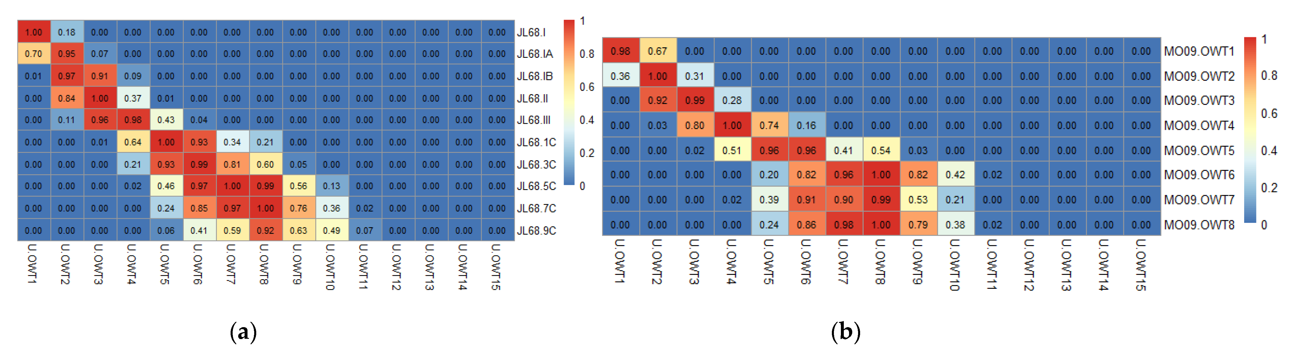
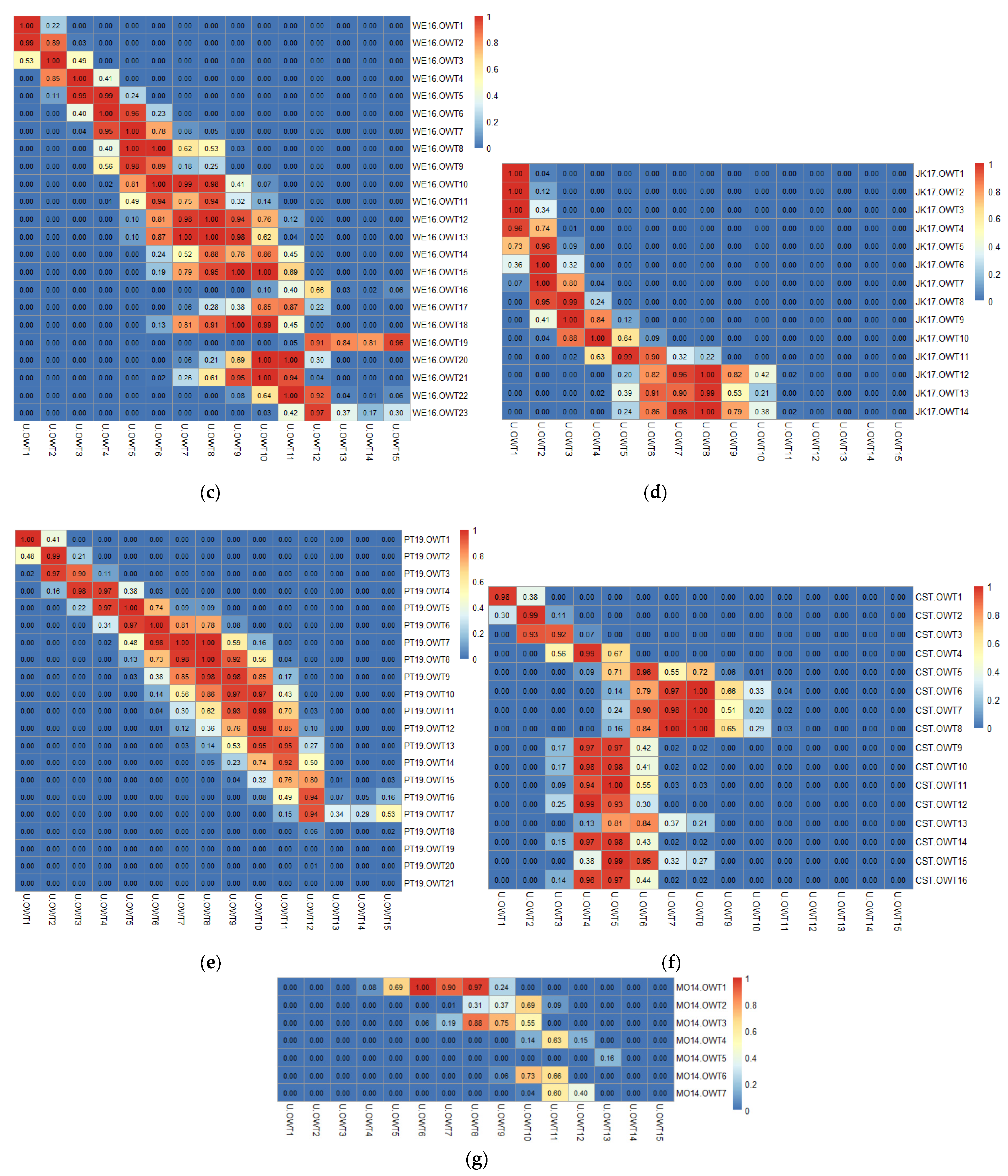
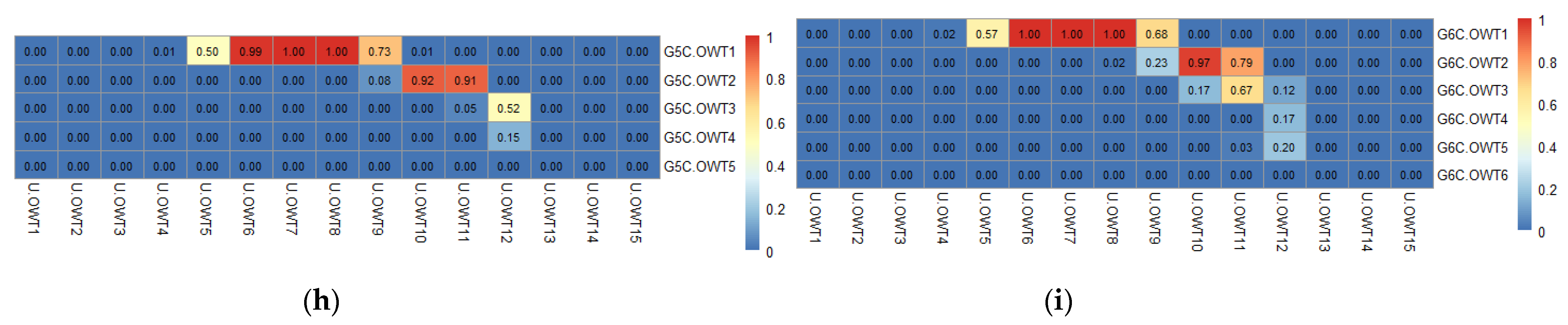
2.3.1. Existing AOP-Based OWT Schemes

In order to compare the U-OWT with other AOP-based OWT schemes and to indirectly prove the rationality of the U-OWT, 9 OWT schemes from the previous studies were selected. They were acquired from Jerlov (1968) [6] (JL68), Moore et al. (2009) [10] (MO09), Moore et al. (2014) [13] (MO14), Wei et al. (2016) [15] (WE16), Jackson et al. (2017) [19] (JK17), Pitarch et al. (2019) [23] (PT19), Coastal [49] (CST), GLaSS 5C [49] (G5C), and GLaSS 6C [49] (G6C). Brief introductions to these OWT schemes appear in Table 1, and the mean reflectance vectors of each OWT class from other OWT schemes are shown in Figure S1. Different OWT schemes had their own reflectance shape and point spread; specifically, the reflectance mean vectors determined the spectral shape, and the covariance matrixes determined the spectral point spread [13]. Considering that it is not easy to compare different point cloud distributions, we calculated the memberships of the reflectance mean vectors from other OWT schemes in the U-OWT context. This method illustrated the relationships between other OWT schemes and the U-OWT scheme to a large extent.
The Jerlov OWT scheme was initially suggested by the form of irradiance transmittance through 1 m of seawater; therefore, the Jerlov water types cannot be directly compared to the U-OWT. Solonenko and Mobley derived the total absorption a(λ) and the total scattering b(λ) for each Jerlov water type in the wavelength range of 300−700 nm [50]. The backscattering ratio B is defined as the backscattering coefficient bb divided by the total scattering coefficient b:
B = b b / b
However, the exact B values for the Jerlov water types were unknown. In the natural world most oceanic particles have backscatter ratios between 0.001 (e.g., very large phytoplankton) and 0.1 (e.g., very small mineral particles) [3]. To derive the bb, we assumed B = 0.001, 0.01, and 0.1 to represent the different scenarios as much as possible. Gordon et al. proposed the relationship between the subsurface remote sensing reflectance rrs(λ) and the inherent optical properties a(λ) and bb(λ) [51],
r r s ( λ ) = 0.0949 b b ( λ ) a ( λ ) + b b ( λ ) + 0.0794 ( b b ( λ ) a ( λ ) + b b ( λ ) ) 2
The semianalytical relationship between the subsurface remote sensing reflectance rrs(λ) and the surface remote sensing reflectance Rrs(λ) proposed by Lee et al. (2002) [52] is as follows:
r r s ( λ ) = R r s ( λ ) 0.52 + 1.7 R r s ( λ )
Following Equations (6)–(8), the Rrs(λ) of all Jerlov water types were obtained, then we interpolated the Jerlov OWT Rrs(λ) to the SeaWiFS multispectral bands and calculated their memberships in the U-OWT context.
For the other OWT schemes (MO09, MO14, CST, G5C, and G6C) displaying with the form of rrs(λ), Equation (8) was applied to convert their water type means rrs(λ) corresponding to different band settings to Rrs(λ). Then, each water type of MO09, MO14, CST, G5C, and G6C was compared with the SeaWiFS 6-band, MERIS 10-band, SeaWiFS 5-band, OLCI 13-band, and OLCI 13-band U-OWT schemes, respectively. Likewise, for the OWT schemes (WE16, JK17, PT19) with the form of Rrs(λ) or nRrs(λ), each water type of WE16, JK17, and PT19 was directly compared with the MODIS-A 8-band, SeaWiFS 6-band, and SeaWiFS 6-band U-OWT scheme, respectively.

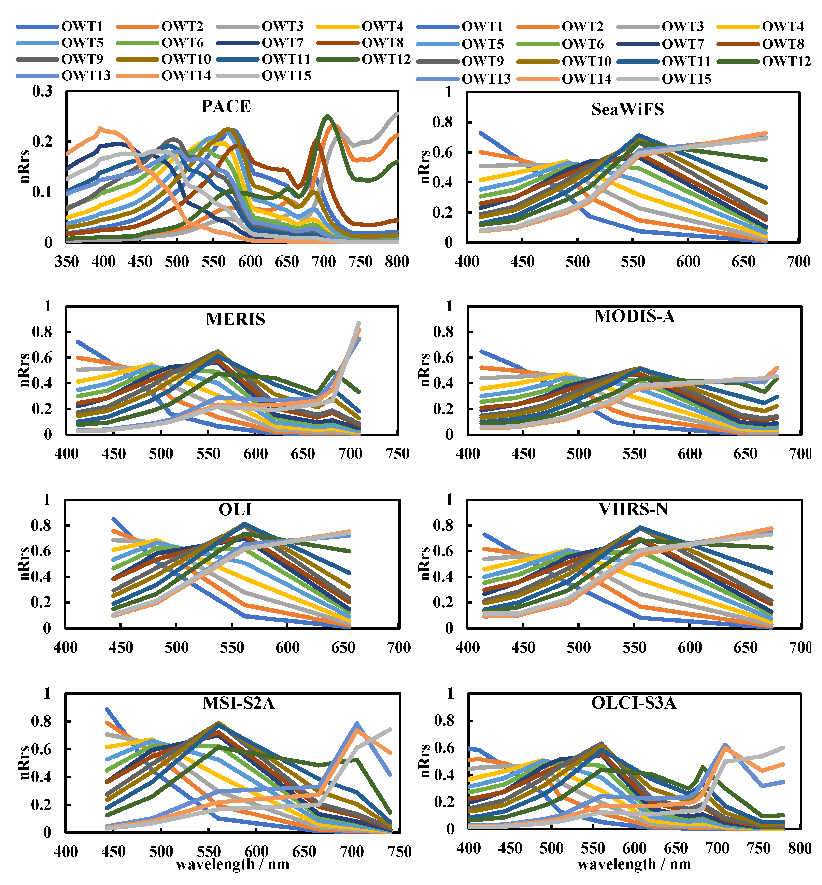
2.3.2. Consistency Evaluation of U-OWT Performance on Different Sensors

The consistency performance of the U-OWT on different multispectral sensors was still unknown. To this end, the IOCCG Hydrolight Synthetic Chla and Rrs(λ) data pairs (sun zenith angle = 30°) were used as a consistent set of evaluation benchmarks for all sensors. Specifically, 75 hyperspectral Rrs(λ) corresponding to Chla = 0.3, 3 and 30 mg/m3 were selected. The above hyperspectral Rrs(λ) were convoluted to different multispectral band settings, then the dominant OWT and average memberships of the U-OWT were calculated to explore the consistency between different sensors. The trophic state indexes (TSIs) corresponding to Chla = 0.3, 3, and 30 mg/m3 were equal to 18.7, 41.4, and 63.9, which represent the oligotrophic, mesotrophic, and eutrophic water states, respectively (see Section 2.4.1).
In addition, two concurrent OLI and OLCI images, which were taken overpassing Pearl River Estuary on 23 October 2017, were selected to evaluate the consistency between the two sensors with the biggest difference in band settings (4 bands for OLI and 13 bands for OLCI) from a spatial distribution perspective. Before the membership and dominant OWT calculations of the above two level 1 images, they were atmospherically corrected using the C2RCC module embedded in the SNAP® platform to transform the top of atmosphere reflectance to the surface remote sensing reflectance (Figure S2).

2.3.3. Sensitivity Analysis of the U-OWT

As a local sensitivity analysis method, the one factor at a time (OAT) method [53] was used in this study to evaluate the robustness of the U-OWT scheme by varying the input Rrs(λ). The Rrs(λ) values in the wavelength ranges 400–500 nm (blue bands), 500–600 nm (green bands), 600–700 nm (red bands), and 700–800 nm (near-infrared bands) were regarded as factors [25]. For the 15 U-OWT Rrs(λ) mean vectors of the multispectral sensors, the perturbation range changed from −100 to 100%, with 10% increments. In this process, the dominant OWT and the memberships of that 15 Rrs(λ) were recalculated to evaluate the robustness of the U-OWT. Three sensors, OLI, MODIS-A and OLCI, were selected to conduct the above sensitivity analysis, which equipped the minimum (4 bands), the medium (8 bands) and the maximum (13 bands) band numbers.

2.4. Other Water Classification Taxonomies

2.4.1. Chla-Based TSI

In this section, the synthetic (SeaWiFS 6 bands for IOCCG) and in situ (SeaWiFS 6 bands for NOMAD and MERIS 9 bands for CCRR) Chla samples, together with their multispectral Rrs(λ) data pairs, were used to determine the relationship between the U-OWT and the water quality parameter (Chla concentration). Meanwhile, the trophic state index (TSI) [34] was used to evaluate the trophic state of the dominant OWT of the U-OWT:
TSI ( C h l a ) = 10 ( 6 2.04 0.68 ln C h l a ln 2 )
where Chla is the concentration of Chla in micrograms per liter. The water trophic state is regarded as oligotrophic, mesotrophic and eutrophic when TSI < 30, 30 ≤ TSI < 50, and TSI ≥ 50, respectively [37].

2.4.2. IOP-Based Classification

Water color classification schemes are primarily based on absorption rather than scattering, as scattering contributes more to brightness but less to color [3]. The seawater absorption coefficient can be subdivided into four principal parts [54]:
a t o t ( λ ) = a w ( λ ) + a p h ( λ ) + a g ( λ ) + a d ( λ )
where atot(λ), aw(λ), aph(λ), ag(λ), ad(λ) are the absorption coefficients of total, pure seawater, phytoplankton, colored dissolved organic matter (CDOM), and non-algal particles (NAPs), respectively. An optical classification based on aph(λ), ag(λ), and ad(λ) was proposed by Prieur and Sathyendranath [54]. For 440 nm, the contributions of phytoplankton, CDOM, and NAP to the total absorption after subtracting the water contribution were defined:
η ( a p h ) = a p h ( 440 ) a t o t ( 440 ) a w ( 440 ) × 100 %
η ( a g ) = a g ( 440 ) a t o t ( 440 ) a w ( 440 ) × 100 %
η ( a d ) = a d ( 440 ) a t o t ( 440 ) a w ( 440 ) × 100 %
At a given wavelength, the ternary plot is a way to illustrate the relative proportions of each absorption subdivision to the total value [55]; it shows how different subdivision constituents dominate absorption [3]. In this study, the absorption spectra corresponding to the 714 raw Rrs(λ) of the PACE synthetic data set were retrieved to explore the relationship between the U-OWT and the absorption properties.

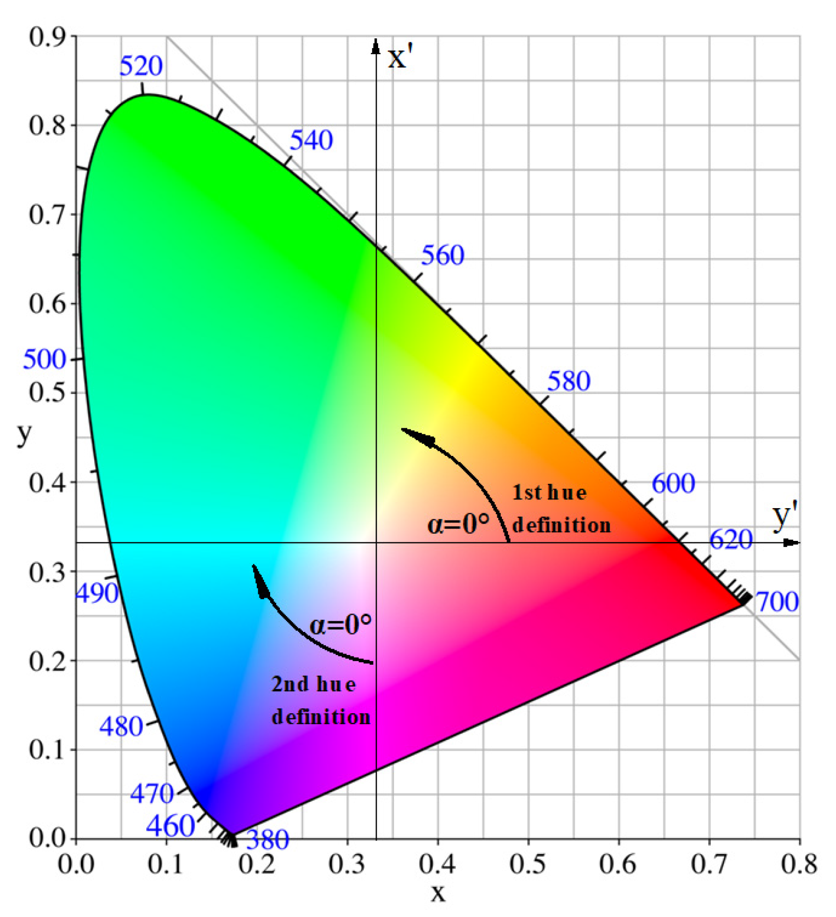
2.4.3. Forel-Ule Scale

In order to explore the relationship between the U-OWT and Forel-Ule Scale, a hue angle and Forel-Ule Index (FUI) retrieval workflow was used for the visible bands of OLCI; the steps are summarized below:
(1)
CIE tristimulus calculation:
X = i = 1 11 x i   R r s ( λ i )
Y = i = 1 11 y i   R r s ( λ i )
Z = i = 1 11 z i   R r s ( λ i )
where X, Y, Z are CIE tristimulus variables, Rrs(λi) denotes the OLCI multispectral remote sensing reflectance spectra, and xi, yi, zi are linear conversion coefficients to calculate the chromaticity values based on OLCI bands (Table A1) [36].
(2)
CIE chromaticity coordinates calculation:
C h r x = X X + Y + X
C h r y = Y X + Y + X
where Chrx and Chry are chromaticity coordinates.
(3)
Hue angle calculation. The hue angle under the Woerd and Wernand (2015) definition (namely the first hue definition) [36] is obtained:
α O L C I = 90 ATAN ( C h r x 1 / 3 ,   C h r y 1 / 3 ) 180 / π
where αOLCI is the hue angle under the first hue definition, ATAN denotes the arctangent function. To reduce the color difference between the hyperspectral true color and the multispectral sensor band setting, a systematic deviation (Δ) is defined as the hyperspectral hue angle αhyper minus the multispectral hue angle, and Δ is the function of the multispectral hue angle [36]. For OLCI sensor:
Δ = α h y p e r α O L C I f ( α O L C I )
If b = α O L C I   /   100 , Δ can be approximated by [36]:
Δ = 12.508   b 5 + 91.635   b 4 249.848   b 3 + 308.656   b 2 165.482   b + 28.561  
Therefore, the corrected hue angle can be obtained:
α h y p e r = α O L C I + Δ
Then, the transformed hue angle under the Wang et at. (2018) definition (namely, the second hue definition) is calculated [37,56]:
α = 270 α h y p e r
The only difference between the first and the second hue definition is that as the hue angle increases, the FUI also increases under the second hue definition, whereas the FUI decreases under the first hue definition (Figure 2). The second hue definition is more coordinated between the hue angle and the FUI. Therefore, the following analysis in this study is under the second hue definition.
(4)
FUI determination. Based on the transformed hue angle, the FUI was calculated using the FUI look-up table (LUT, Table A2): the transformed hue angle was pointed toward the nearest LUT 21 class standard hue angle, and the FUI corresponding to that standard hue angle was what we wanted [57].

2.5. Global Ocean Applications of the U-OWT

The U-OWT scheme was applied to the ESA-OC-CCI v4.2 Rrs Monthly Climatology (1998–2019) data sets to explore the global seasonal variability of ocean optical classes. Specifically, the dominant OWT and memberships of each U-OWT class for each month were calculated. For brevity, the memberships of January, April, June, and September are shown in this paper, to represent the seasonal variability. What is more, the monthly Shannon index of the U-OWT normalized memberships was calculated to evaluate the ocean optical diversity [14,20]. For a given bin:
H = i = 1 N P i   ln ( P i )  
where H is the Shannon diversity index, Pi is the normalized membership of each optical water type of the U-OWT, and N denotes the number of optical classes; here, N = 15. If the 15 optical water types have the same membership, i.e., 1/15, H reaches a maximum value of ln(15) = 2.7, which means the maximum optical diversity; in contrast, if one bin is composed of only one optical class, H reaches a minimum value of 0, which indicates the minimum optical diversity.

3. Results

3.1. U-OWT Cluster Analysis

The mean normalized remote sensing reflectances nRrs(λ) of 15 U-OWT classes for the PACE hyperspectral sensor and different multispectral sensors are depicted in Figure 3. For the original hyperspectral U-OWT scheme, the nRrs(λ) spectra of different classes were well separated from others. The peaks of OWT1-15 increased from blue wavelength to near-infrared wavelength: the nRrs(λ) peaks of OWT1-3 were located near 410nm; the nRrs(λ) peaks of OWT4-6 were located near 490 nm; the nRrs(λ) peaks of OWT7-12 were located near 560 nm; the nRrs(λ) peaks of OWT13-15 were 700–800 nm. In addition, another spectral peaks for OWT1-12 classes was observed near 685 nm, and the value of this peak increased gradually from OWT1 to OWT12. The 685 nm mark is often used in the calculation of fluorescence line height (FLH) and maximum Chlorophyll index (MCI), which are the indicators of the biological activity of phytoplankton [58]. Therefore, the increasing 685 nm peak values may imply gradually stronger phytoplankton signals from OWT1 to OWT12. OWT13-15 did not show obvious 685 nm peaks, and we deduced that they were turbid water types and were more influenced by suspended sediments and organic particles [10], causing the light availability to decrease for the primary producers, thus limiting Chla concentration [23].
As the set of U-OWT schemes of multispectral sensors were converted from the PACE hyperspectral scheme, the shape and magnitude of the multispectral U-OWT nRrs(λ) were similar to the original hyperspectral scheme, especially for the multispectral sensors with relatively more band numbers, e.g., OLCI and MERIS. On the contrary, the U-OWT schemes of the multispectral sensors with fewer band numbers lost some spectral characteristics of the original hyperspectral scheme, e.g., OLI, which had only four visible bands.

3.2. Reliability of the U-OWT

3.2.1. Inter-Comparison with Other AOP-based OWT Schemes

Regarding OWT schemes aiming at global ocean classification, including JL68, MO09, WE16, JK17, and PT19, they showed good correspondence with the U-OWT. Each class corresponded to one or more specific U-OWT classes, and the correlations were relatively high (membership > 0.5). The OWT classes of JL68, MO09, and JK17 approximately corresponded to OWT1-10 of the U-OWT successively; however, they had no corresponding classes with OWT11-15 of the U-OWT. Specifically, JL68, MO09, and JK17 appeared to classify oligotrophic water classes redundantly, i.e., they had several OWT classes corresponding to OWT1-4 of the U-OWT; while for the mesotrophic and eutrophic waters, one of their OWT classes often corresponded to several OWT5-10 classes of the U-OWT. It is worth noting that when the backscattering ratio B varied, the above phenomena were still valid for the JL68 scheme. As for WE16, its OWT classes well corresponded to OWT1-15 of the U-OWT successively, though there was only WE16.OWT19 corresponded to OWT13-15 of the U-OWT. OWT1-17 of PT19 were well related to OWT1-12 of the U-OWT; however, OWT18-21 of PT19, i.e., the CDOM-dominated classes [23], had no correspondence with the U-OWT (Figure 4). In general, the U-OWT showed good comparability with other global ocean-aimed OWT schemes, which indirectly proved the representativeness and reliability of the U-OWT.
Though the U-OWT had good correlation with other ocean-aimed OWT schemes, the correlation with the OWT schemes for the inland and coastal waters (including MO14, CST, G5C, and G6C) was not significant. Many classes of these inland and coastal water-aimed OWT schemes did not have classes corresponding to the U-OWT (Figure 4).

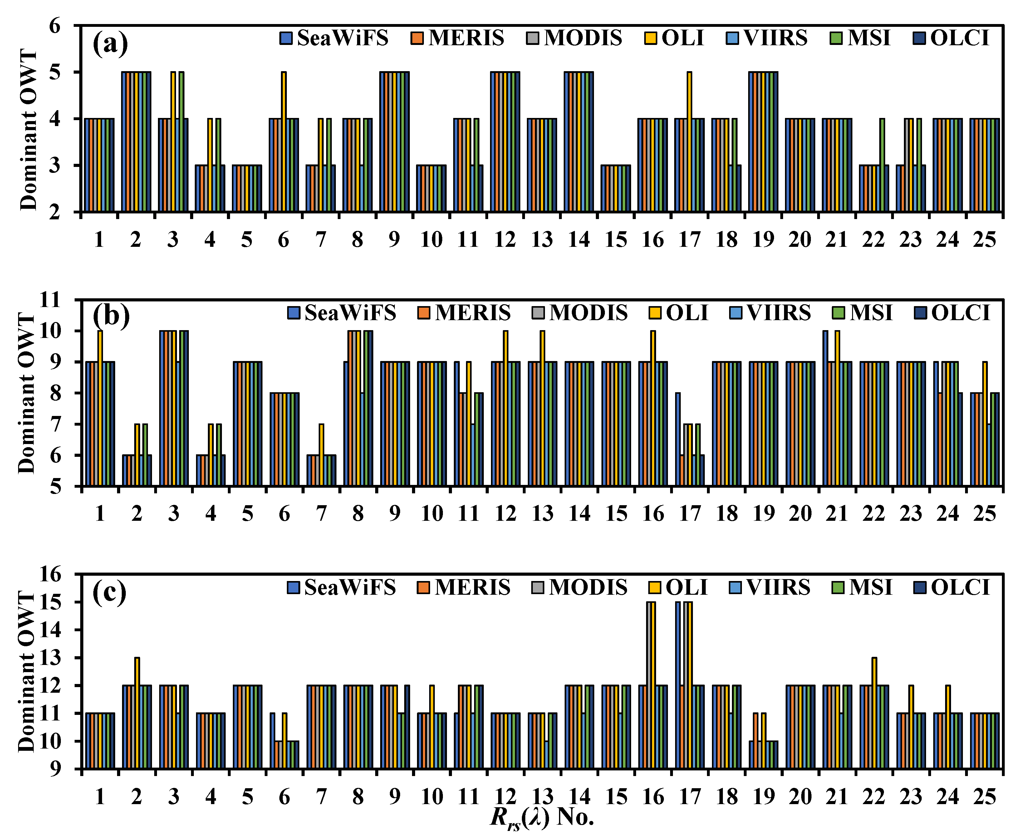
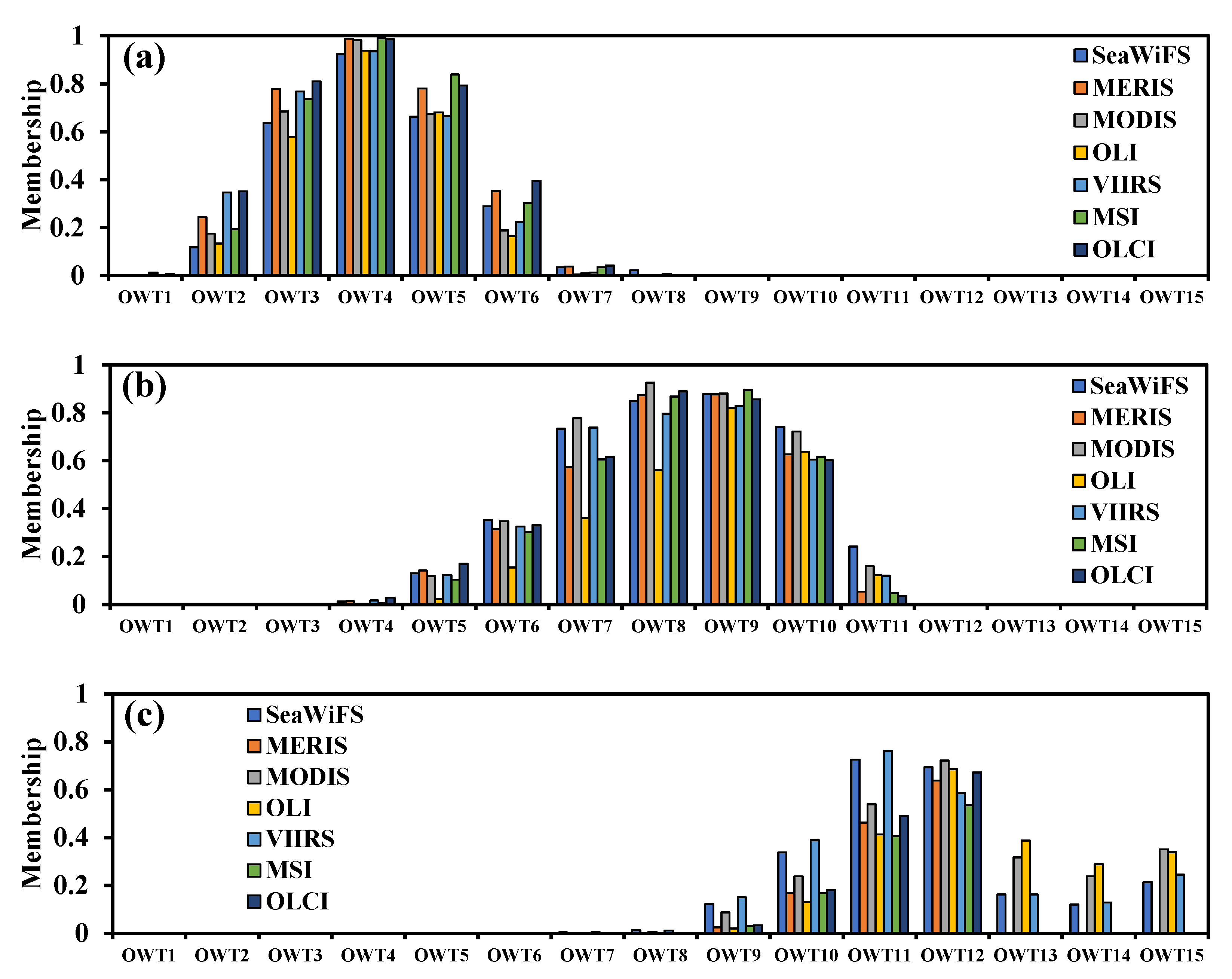
3.2.2. Consistency Analysis between Different Multispectral Sensors

For the 75 IOCCG oligotrophic, mesotrophic and eutrophic synthetic spectra (each trophic state had 25 spectra), their dominant OWT (Figure 5) and average OWT memberships (Figure 6) under the U-OWT context, which were calculated between different multispectral sensors, showed relatively good consistency, although the dominant OWT calculated under a few sensors’ U-OWT schemes was not equal to the majority counterparts, the deviations were fewer than three dominant OWT classes.
For the two concurrent OLI and OLCI images, their spatial distribution patterns of the OWT1-12 memberships were similar, although the membership values around the rims of OWT1-9 were higher in the OLI image (Figure 7a), and the membership values around the rims of OWT10-12 were higher in the OLCI image (Figure 7b). From the perspective of the dominant OWT, both the OLI and OLCI images had similar spatial distributions and values for the oligotrophic (OWT1-5) and eutrophic (OWT9-12) water types, however, there was significant inconsistency in the spatial distributions in the mesotrophic water types (OWT6-8) (Figure 8). The band settings of different multispectral sensors, specifically the band numbers and the band locations, may have affected the U-OWT performance between sensors.

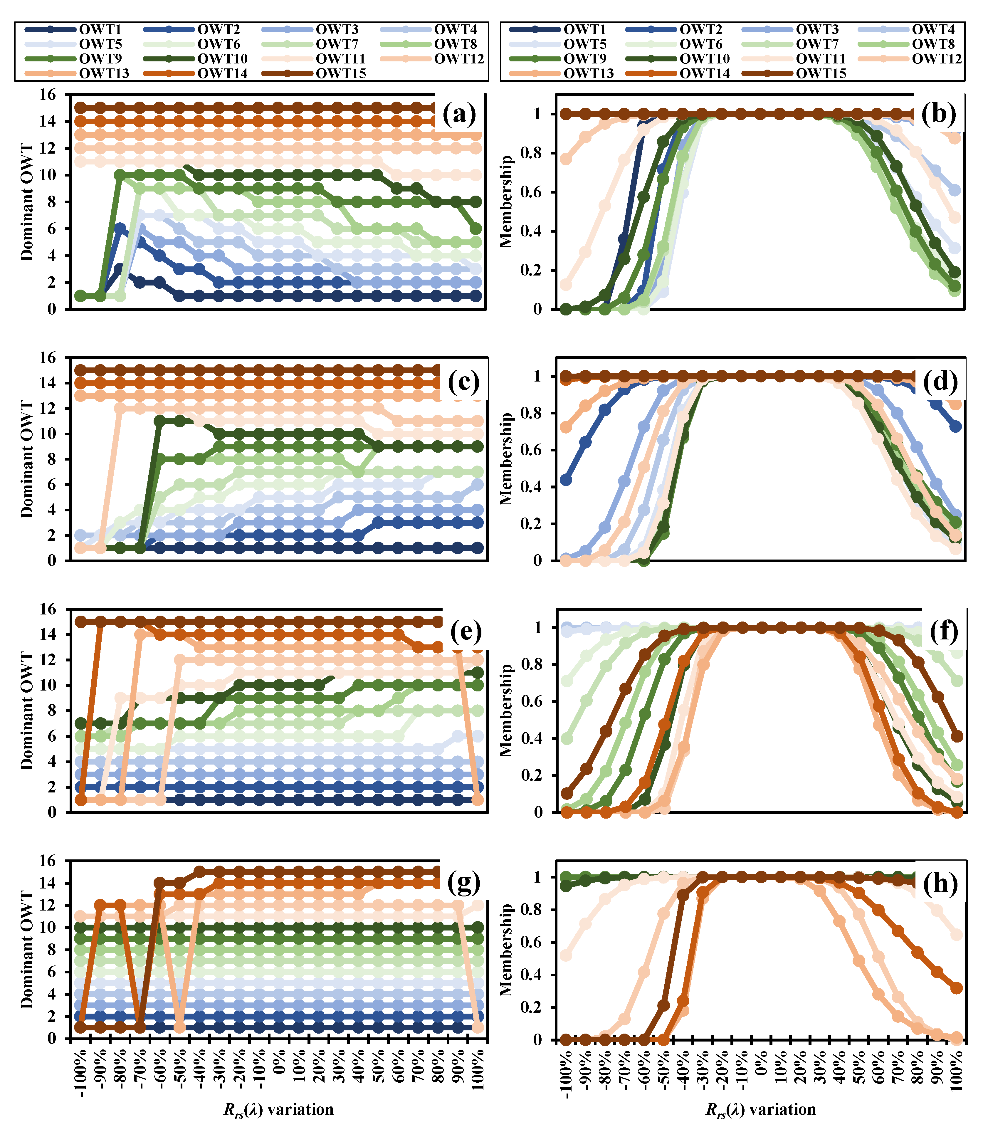
3.2.3. Sensitivity Analysis

The local sensitivity of the U-OWT schemes corresponding to OLI, MODIS, and OLCI are seen in Figures S3 and S4, and Figure 9, respectively. Taking OLCI as an example, the perturbation of Rrs values in the wavelength range of blue bands (400–500 nm) mainly affected the oligotrophic and mesotrophic water classes (OWT1-8), in terms of the dominant OWT and the membership values. The increase in blue band Rrs values could have decreased the OWT class numbers, while the decrease in blue band Rrs values could have increased the OWT class numbers. Additionally, the perturbations of the green bands (500–600 nm), red bands (600–700 nm), and near-infrared bands (700–800 nm) Rrs values mainly affected the mesotrophic (approximately OWT5-10), eutrophic (approximately OWT9-12), and over-eutrophic (approximately OWT13-15) U-OWT classes, respectively. In addition, according to the membership sensitivity analysis, the OLCI U-OWT scheme can endure nearly ±30% Rrs(λ) perturbations on different wavelength ranges.
The above phenomena were also detected in the OLI and MODIS U-OWT schemes. However, the OLI and MODIS U-OWT schemes could only endure nearly ±10 and ±20% Rrs(λ) perturbations on different wavelength ranges, respectively. That may be due to the fewer band numbers of these two sensors. Generally, the sensitivity of the U-OWT was influenced differently by the OWT classes, sensor types, and wavelength ranges [25].

3.3. Relationships to Other Water Type Taxonomies

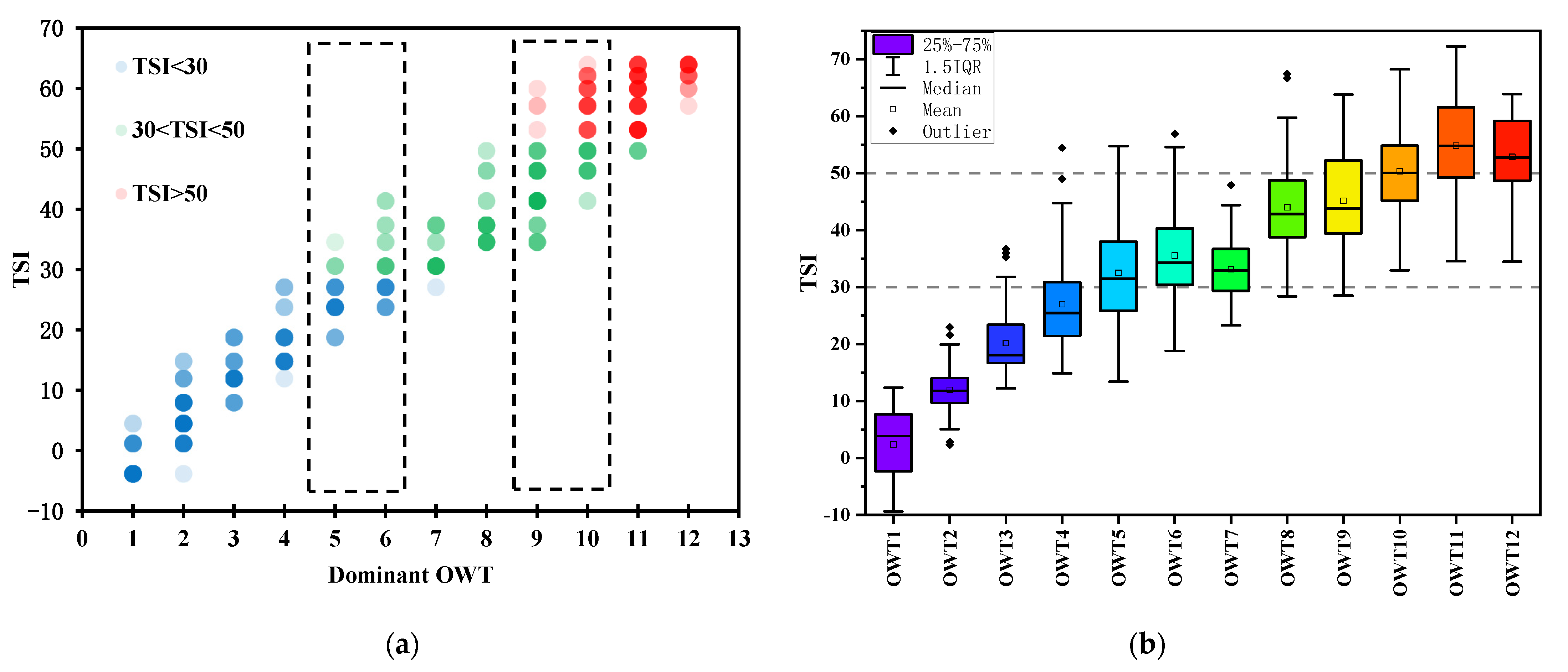
3.3.1. Relationship to the Chla-Based TSI

The synthetic and in situ data showed that each U-OWT class corresponded to a different Chla concentration range, whose values had an exponential increment (Figure S5). The in situ measurements were globally located, and the high-numbered OWT samples were mainly in the coastal regions, while the low-numbered OWT samples were mainly in the open ocean waters (Figure S6). The Chla concentrations of oligotrophic water classes (OWT1-4), mesotrophic water classes (OWT5-9), and eutrophic water classes (OWT10-12), were mainly in the ranges of 0.01–1, 1–10, and >10 mg/m3, respectively. The synthetic and in situ data did not contain enough OWT13-15 spectra samples; thus, the Chla concentrations of OWT13-15 are not shown here. However, it was expected that the Chla concentrations of OWT13-15 were greater or roughly equal to OWT10-12. In addition, the Chla concentrations of the adjacent OWT classes had overlapping intervals, which indicated that the Chla inversion algorithms corresponding to the adjacent OWT classes can be weighted blended based on memberships to improve the Chla inversion accuracy in the full concentration range.
We regarded the water bodies with TSI < 30, 30 < TSI < 50, and TSI > 50 as oligotrophic, mesotrophic, and eutrophic states, respectively [37]. From the analysis of the synthetic data set, OWT1-4 of the U-OWT represented oligotrophic waters, OWT5-6 were transitional between oligotrophic and mesotrophic states, OWT7-8 were mesotrophic waters, OWT9-10 were transitional between mesotrophic and eutrophic waters, and OWT11-12 were eutrophic waters (Figure 10a). The above phenomena were also confirmed by the in situ observations (Figure 10b). Although in the synthetic and in situ data sets, there were not enough Rrs(λ) spectra and Chla pairs corresponding to OWT13-15 classes, these water classes were expected to belong to eutrophic waters.

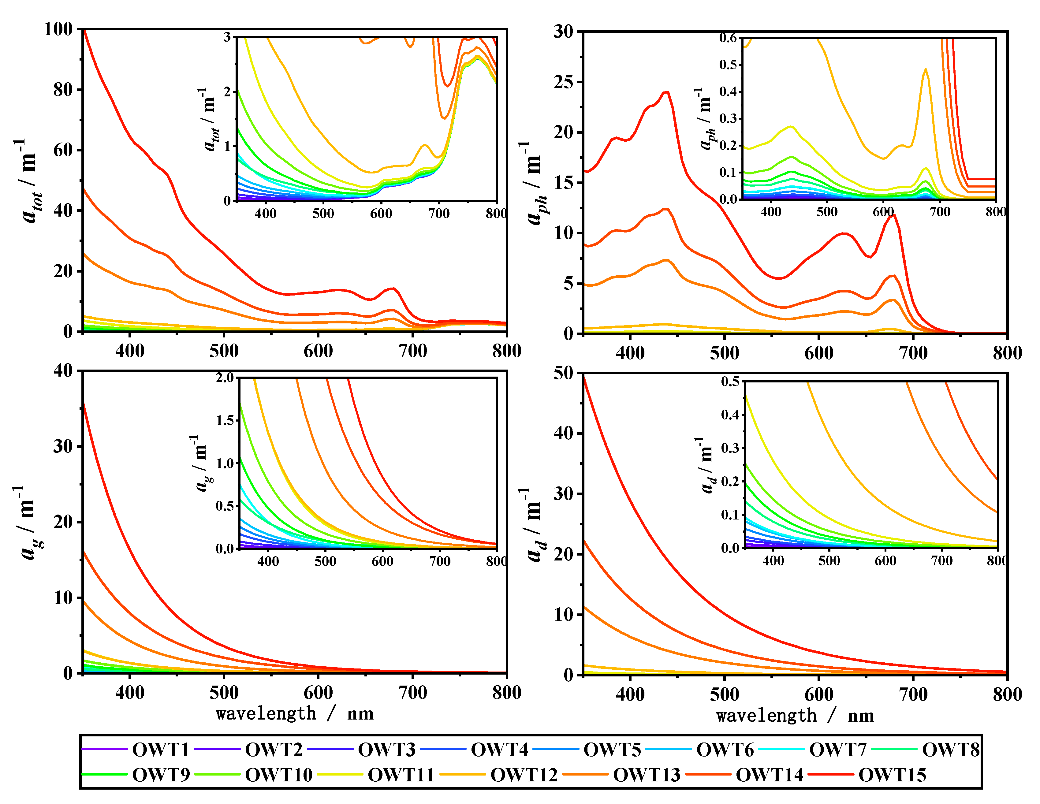
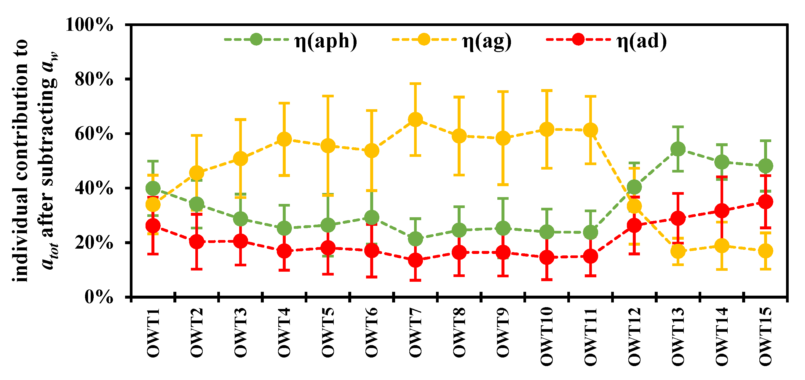
3.3.2. Relationship to the Absorption Properties

The mean atot(λ), aph(λ), ag(λ), and ad(λ) spectra of the PACE synthetic data for each U-OWT class appear in Figure 11, and they were highly spectrally dependent. The magnitude of absorption varies linearly with the concentration of the absorbing material [3]; therefore, the exponential increase in the absorption spectra may illustrate the increasing absorption materials for the U-OWT classes. Because of the presence of Chla, two peaks of the aph(λ) spectra were in the blue and red wavelength regions [3], one was near 440 nm, and another was near 680 nm. The ag(λ) values were high in the blue wavelength and decreased exponentially to the red regions. The ad(λ) spectra were very similar to the ag(λ), but with a more gently decreasing slope. The total absorption was composed of pure water and three individual absorption components; thus, it had an exponential decreasing slope and two peaks around the blue and red regions.
Similar to a ternary plot of the individual absorption contributions, a line chart depicting the contributions of aph(440), ag(440), and ad(440) to total absorption after subtracting water contribution is in Figure 12. From OWT1 to OWT11, η(aph) and η(ad) decreased gradually, while η(ag) increased gradually and exceeded η(aph) and η(ad). The transition was at OWT12; in this water class, η(aph) and η(ad) increased while η(ag) decreased. At OWT13-15, the comparison between the individual contributions was η(aph) > η(ad) > η(ag).

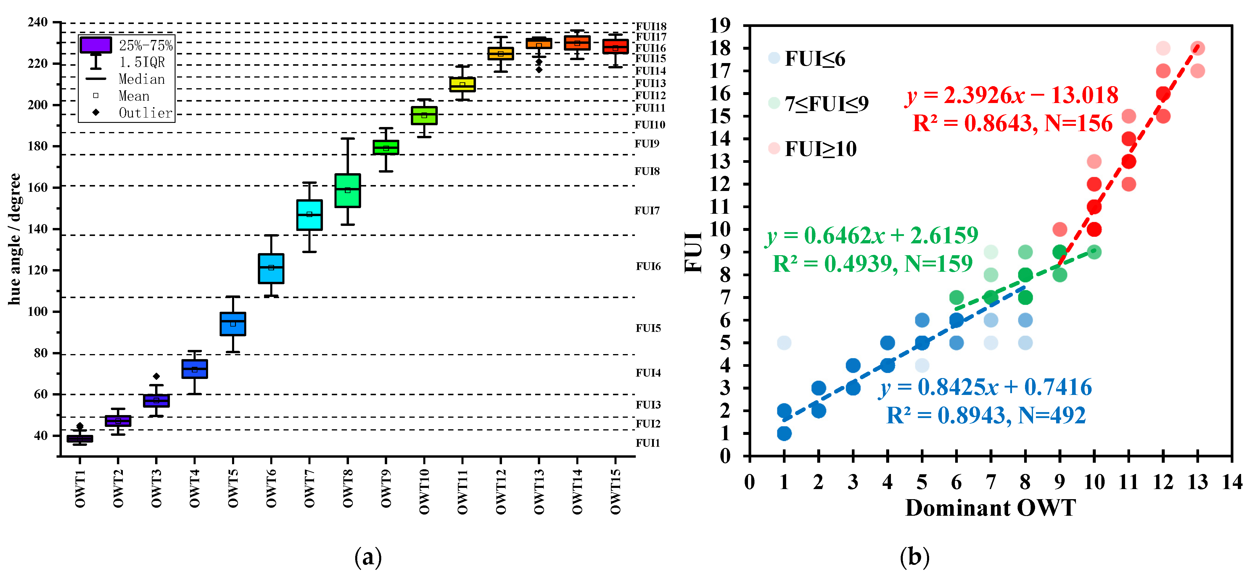
3.3.3. Relationship to the Forel–Ule Scale

Analysis of the IOCCG synthetic data showed that in the oligotrophic water types, i.e., OWT1-6, one U-OWT class roughly corresponded to one FUI class; in the mesotrophic water types, i.e., OWT7-10, one U-OWT class often corresponded to several FUI classes; in the eutrophic water types, i.e., OWT11-15, one FUI class corresponded to several U-OWT classes (Figure 13a). In other words, for the purpose of water quality assessment, the distinguishable abilities of the U-OWT and FUI were equal in oligotrophic waters, FUI was better in mesotrophic waters, while the U-OWT was better in eutrophic waters. The in situ data from the global oceans and offshore China also confirmed the case (Figure 13b).
In addition to the spectral analysis of comparison between the U-OWT and the FUI, one OLCI image overpassing the Pearl River Estuary was processed for the spatial consistency analysis of the U-OWT and FUI. Figure 14 shows that the dominant U-OWT class had a spatial pattern that was high consistent with the FUI, especially in terms of the boundary distribution of the corresponding OWT and FUI classes. Similar to the spectral consistency analysis, the FUI had a better ability to distinguish in mesotrophic waters than the U-OWT. For instance, in the waters off Hong Kong, the U-OWT only classified waters into one class, i.e., OWT8; however, the FUI classified the same areas into three classes, i.e., FUI7-9. The U-OWT has its limitations; even so, its dominant OWT classes can potentially be regarded as water quality indicators that are as useful as the FUI.

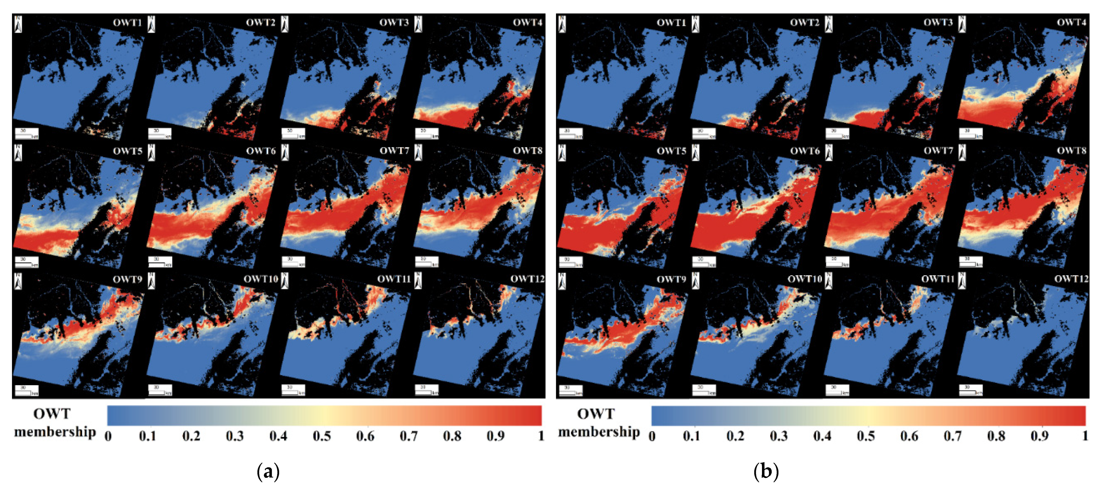
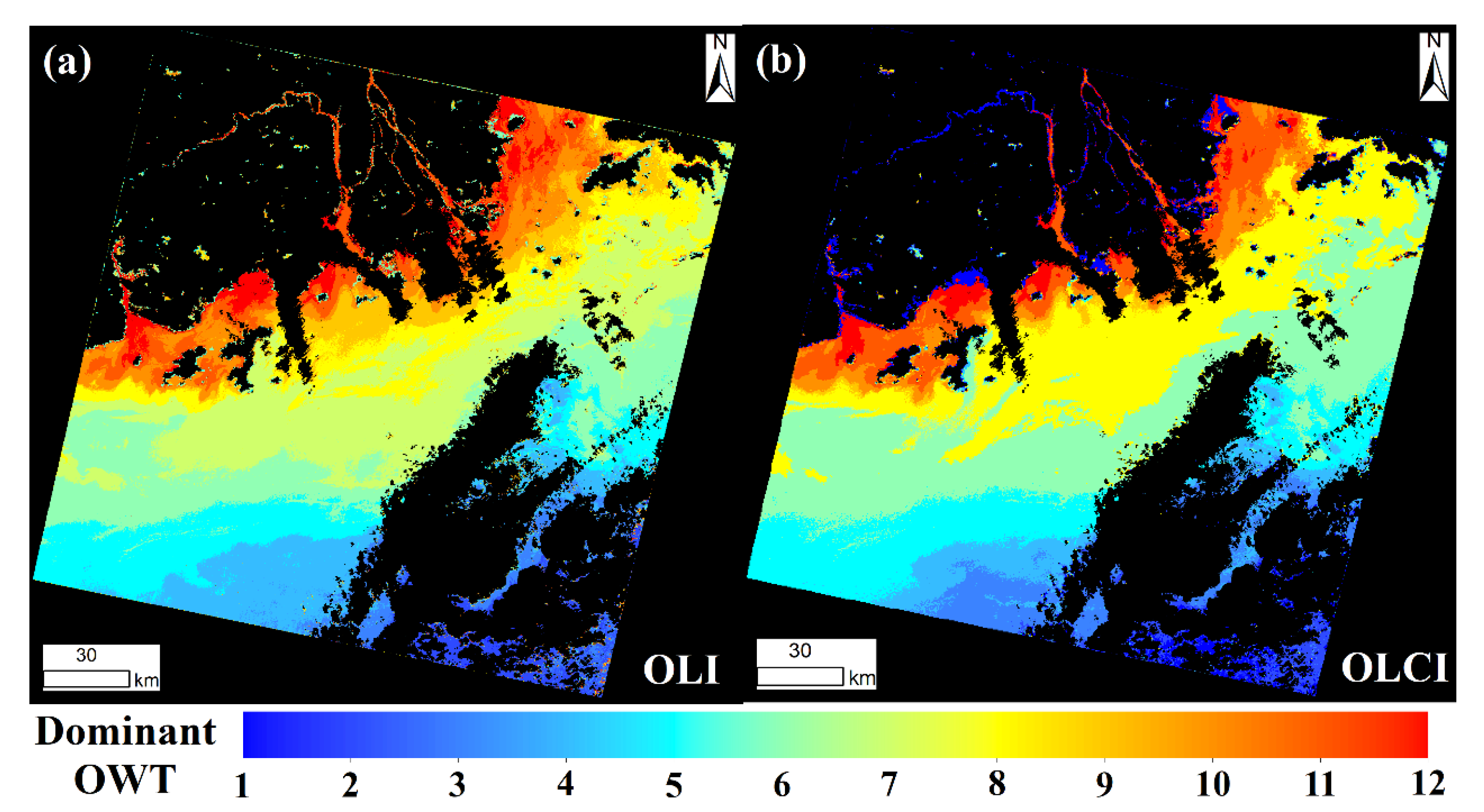
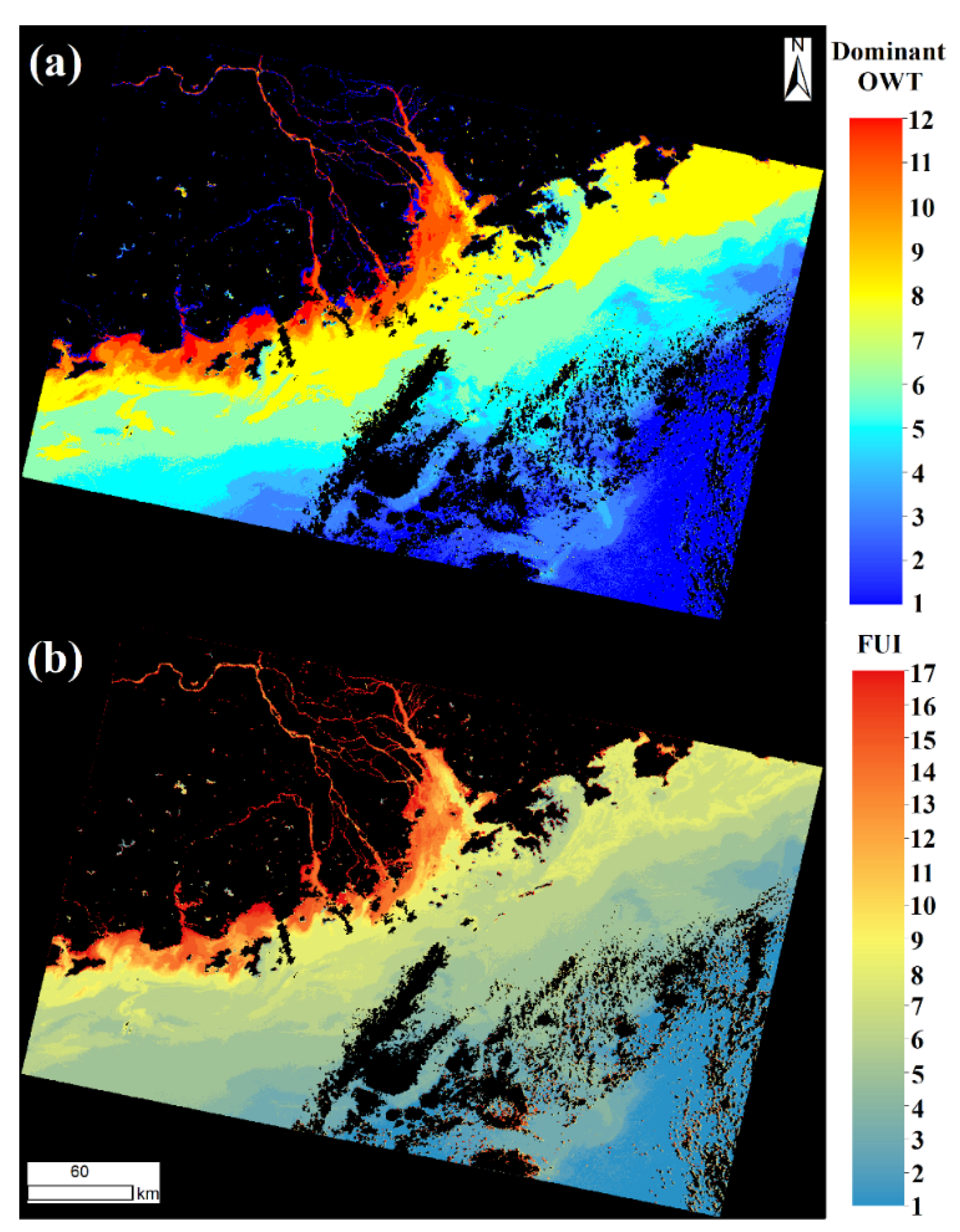
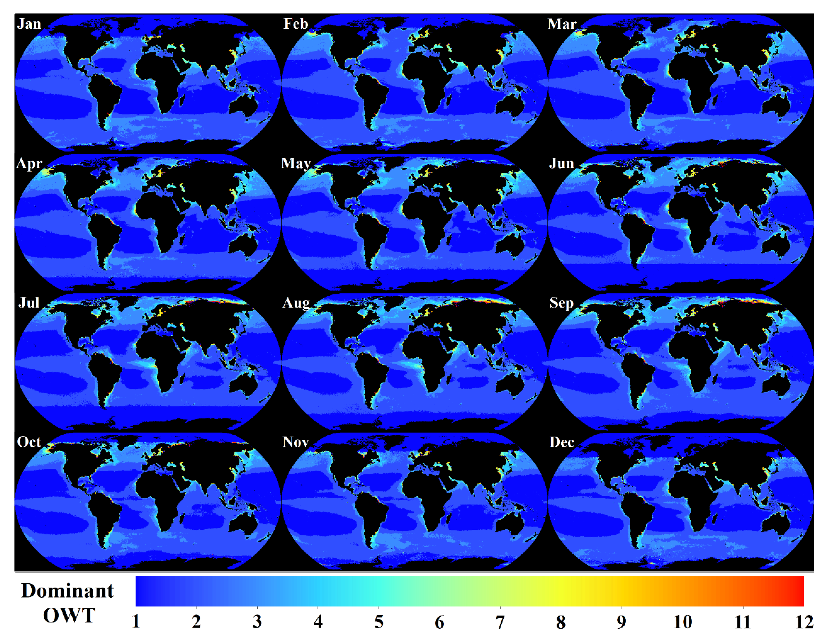
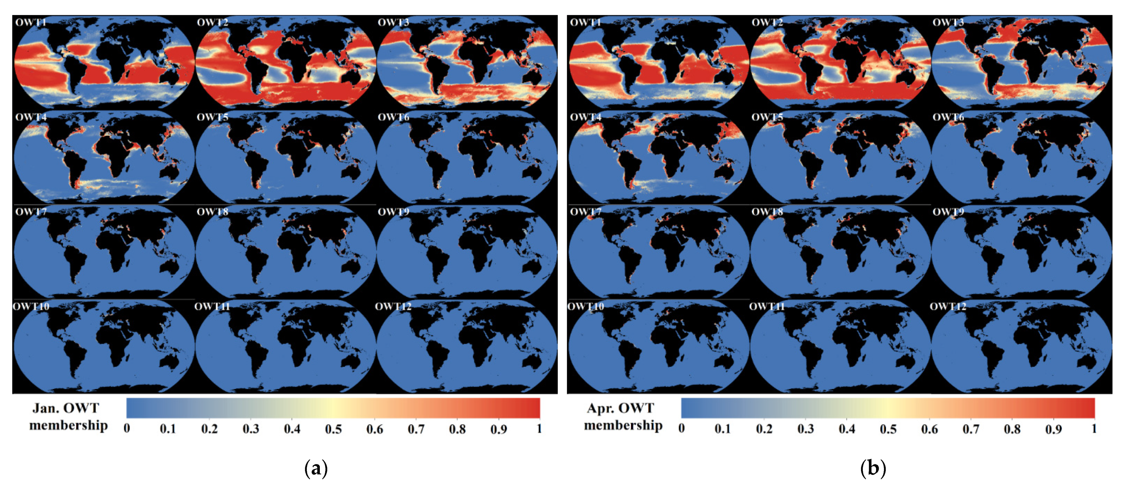
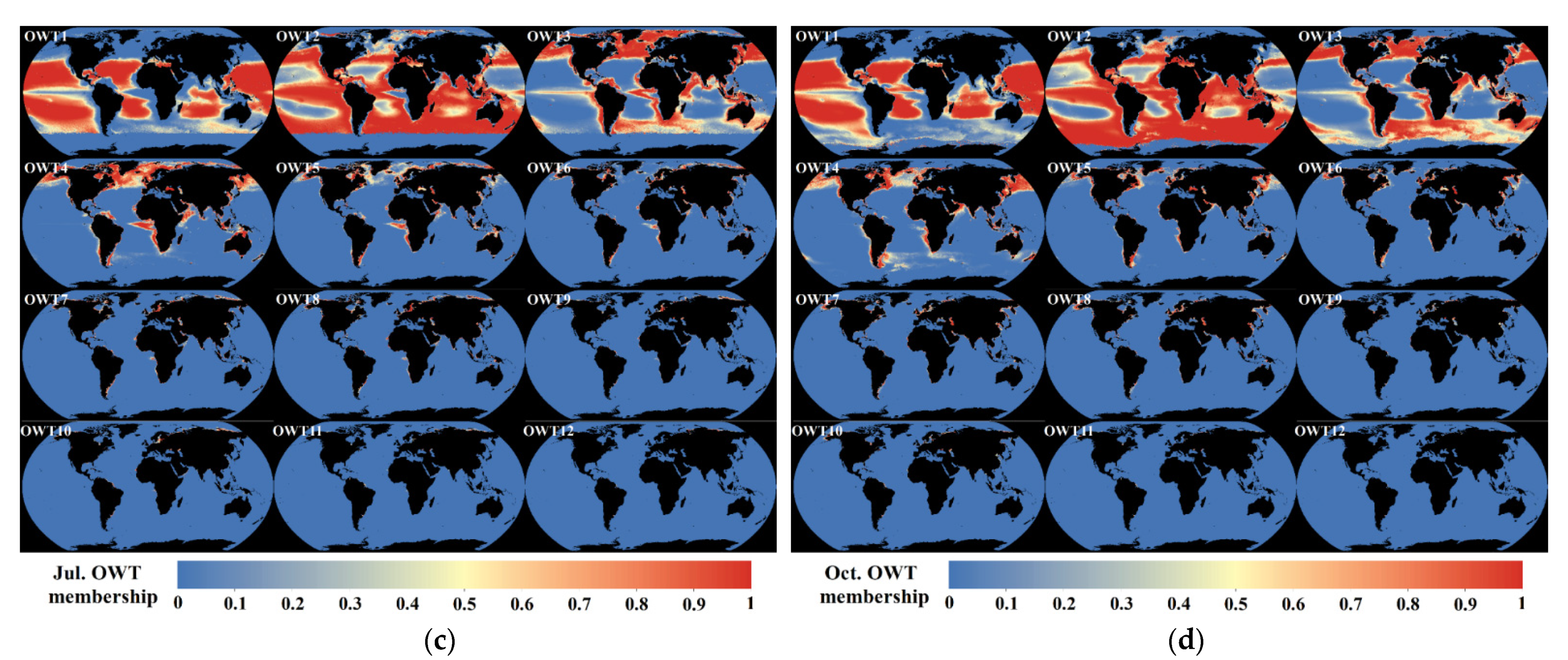
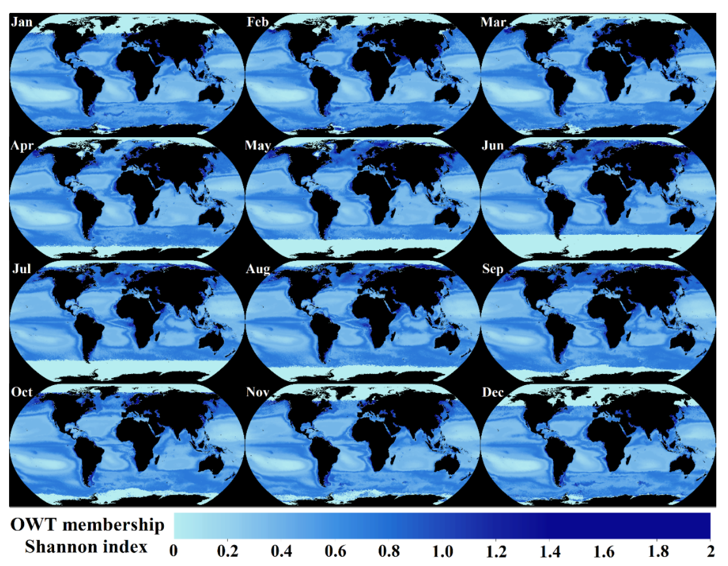
3.4. Global Applications of the U-OWT

The U-OWT scheme was applied to the level-3 ESA-OC-CCI climatology monthly Rrs data to obtain the global oceanic dominant OWT (Figure 15), monthly OWT memberships (Figure 16), and Shannon indexes of normalized memberships (Figure 17). The dominant OWT and memberships showed that most ocean waters were occupied by the two clearest water classes, i.e., OWT1 and OWT2. In addition, the OWT1 ocean regions corresponded to the subtropical gyres surrounded by the OWT2 waters. The monthly variations in subtropical gyres over the past 20 years were obtained: the subtropical gyres in the Northern Hemisphere had a smaller area in January (Northern Hemisphere winter) than in July (Northern Hemisphere summer), while the subtropical gyres in the Southern Hemisphere had a larger area in January (Southern Hemisphere summer) than in July (Southern Hemisphere winter). The OWT classes belonging to mesotrophic and eutrophic waters were mainly located off the shores, including China coastal waters, Red Sea–Persian Gulf, West Africa coastal waters, North Sea–Baltic Sea, East Coastal waters of the United States, Caspian Sea, Black Sea, Argentine Sea, Bering Strait, etc. More details of these coastal areas must be studies in the future. Generally speaking, the closer to the coast, the higher the eutrophic degree of the water bodies. The optical properties of some offshore areas were the result of land–sea interaction. The coastal waters were affected both by runoffs from land sources and by marine factors such as currents and tides.
The ocean optical diversity was observed from the Shannon index; the higher Shannon index indicated higher diversity in the OWT classes, and vice versa. The Shannon index appeared to be relatively high in the transition areas between different dominant OWT classes, and this phenomenon was especially obvious in the edge areas of gyres. As the optical diversity was related to the biological diversity [14,20], further studies are needed to explore the bio-optical properties of the U-OWT Shannon index.

4. Discussion

4.1. How Many Optical Water Types in the World?

According to the Section 3.2.1, the AOP-based OWT schemes which were designed for inland and coastal waters, including MO14, CST, G5C and G6C, did not show good consistency and compatibility with the U-OWT. We speculated that these optically complex water-aimed OWT schemes may contain some unique water types, which the U-OWT does not yet include. At the same time, several ocean-aimed OWT schemes, including JL68, MO09, WE16, JK17, and PT19, were quite compatible with the U-OWT, and most of their water classes could be explained by OWT1-12 of the U-OWT. However, compared to the U-OWT scheme, other ocean-aimed OWT schemes had relatively more oligotrophic water classes and fewer mesotrophic and eutrophic water classes. From the authors’ point of view, one of the most important applications of the optical water classification is in the class-specific algorithms blending for the in-water constituents, such as Chla and total suspended substance (TSS). The coastal and inland waters are more optically complex than the oceanic waters, and some conventional inversion algorithms developed for the clear oceanic waters do not perform well in these turbid waters; thus, class-specific algorithms are urgently needed for these mesotrophic and eutrophic waters. Previous ocean- aimed OWT schemes largely relied on huge in situ and remote sensing spectra samples, and the clear water spectra occupied large proportions of their clustering samples, which affected the water class clustering processes and led to more clear water types in the final OWT schemes. The U-OWT was based on the synthetic spectra, which did not contain repeated spectra samples. Therefore, the U-OWT was not affected by the occurrence frequency of spectra, and more turbid water types could be distinguished, and the optical properties of the optically complex waters could be more comprehensively represented by the U-OWT.
In general, the optical water type numbers of most AOP-based oceanic schemes were between 8 and 23, while the optical water type numbers of most inland and coastal aimed schemes were between 3 and 15. Although the water type numbers of most OWT schemes were determined by the mathematical methods, some trade-offs must be considered: on the one hand, too few classifications may not fully reflect the spectral characteristics of different water bodies; on the other hand, too many classifications will reduce the efficiency of OWT calculation, especially when involving many spectra or satellite data. According to the sensitivity analysis of the U-OWT, OWT1-12 classes were mainly distinguished by the visible wavelength, while the OWT13-15 classes were mainly distinguished by the near-infrared region. The OWT13-15 classes had relatively high nRrs(λ) magnitude in 700–800 nm, which indicated that these water types were highly turbid. Because of the insufficient in situ samples corresponding to the OWT13-15 classes, their bio-optical properties were not fully explored in this study. In highly turbid coastal and estuarine waters, optical variability can be determined for wavelengths longer than 670 nm and cannot be captured by a sensor like SeaWiFS [14]. However, for some satellite instruments that are equipped with near-infrared bands, such as MERIS, MSI and OLCI, they can well detect the highly turbid water types; thus, the OWT13-15 classes of the U-OWT scheme may be more distinguishable using these sensors.
Some previous AOP-based OWT schemes were compared with the U-OWT. However, because of the difficulty in obtaining the raw OWT spectra data, some OWT schemes proposed by previous literatures were not included in such comparisons, such as Vantrepotte et al. [11], Shi et al. [12], Mélin and Vantrepotte [14], Ye et al. [16], Hieronymi et al. [18], Monolisha et al. [20], Spyrakos et al. [21], Uudeberg et al. [25], Xue et al. [26], Zhang et al. [27], Balasubramanian et al. [28], and da Silva et al. [29] The adaptability of the U-OWT in inland waters also deserves to be explored, and some unique OWT classes for inland waters may be added to the present U-OWT scheme in the future.

4.2. Unification of Different Water Type Taxonomies

One of the most intuitive water type taxonomies is the multivariate combination of in-water constituents, such as phytoplankton, detritus, CDOM, and sediment. These in-water constituents can be further subdivided into diverse groups, according to the species, sizes, shapes, builds, etc. [3]. However, accurate and synoptic in situ measurement of the in-water constituents is difficult. Thus, from a remote sensing perspective, IOPs and AOPs can be regarded as the indirect indicators of water properties. The absorption and scattering (backscattering) are the most important IOPs, and they are dependent on the in-water constituents. Taking the radiative transfer model as a bridge, different kinds of AOPs, such as ocean color, radiances, and reflectances can be expressed as the functions of IOPs, and vice versa [59]. Likewise, from in situ or remote sensing observations, in-water constituents can be inversely modeled by AOPs [60]. In general, the interrelationships between AOPs, IOPs, and in-water constituents are explicit. To date, many commonly used water type taxonomies are based on AOPs, IOPs, or in-water constituents, such as the fuzzy logic classification of AOPs spectra, the Forel–Ule Scale, the absorption ternary plot, and the Chla-based TSI. However, the interrelationships between these water classification systems are still ambiguous. To the best of our knowledge, there is no consensus on a universal fuzzy logic AOP-based OWT scheme, and this may hinder the further comparison and integration of different kinds of water type taxonomies. Though different water classification systems have their own characteristics and application scopes, the compatibility of these water type taxonomies is helpful for their inter-comparison and mutual-conversion.
In addition to the Chla-based TSI and the individual absorption proportions, the U-OWT showed high coordination with the Forel–Ule Scale. As the Forel–Ule Scale is known for its applicability to global ocean and inland waters, thus, the U-OWT was indirectly proven to have the potential to be applied globally. In essence, this indicated that the core components of the U-OWT fuzzy logic classification scheme—OWT class mean nRrs vectors and covariance matrixes, were well suitable. At the same time, the U-OWT also showed its difference from and superiority to the Forel–Ule Scale: the FU scale mainly relies on the visible wavelength; thus, it cannot distinguish the spectral characteristics on near-infrared bands, where optically complex waters have non-negligible signals [60]. However, the eutrophic water classes (especially OWT13-15) of the U-OWT can distinguish those optically complex waters. Meanwhile, the fuzzy logic OWT scheme is a bridge and intermediary with many application fields (see Section 4.3); thus, it is expected the U-OWT will have a wider applicative perspective.

4.3. Future Prospects of the U-OWT

Broader applications of the U-OWT can be explored based on the direct U-OWT calculation indicators—OWT membership, OWT normalized membership, total membership, and dominant OWT. One obstacle to the promotion of the fuzzy logic OWT method is that there are few ready-made tools; thus, the authors of this study developed a freely distributed U-OWT calculation tool, and all the above direct OWT indicators can be calculated by the readers. Some indirect OWT parameters derived from the direct OWT indicators are also valuable, such as the Shannon index of the normalized membership.
The fuzzy logic OWT framework was initially introduced by Moore et al. [8], and it has been widely used in bio-optical algorithms blending, such as Chla [11,15,16,22,30] and TSS [28]. In optically complex waters, it is difficult to inverse in-water constituents over entire concentration ranges, and it may be more realistic to use a series of branching algorithms to deal with this problem, rather than a single, all-purpose algorithm [60]. The fuzzy logic OWT schemes can seamlessly integrate such a series of branching inversion algorithms of different water classes, the membership-weighted blending retrievals from the class-specific algorithms showed smooth and continuous patterns [8], which were superior to some conventional means. In the field of IOPs inversion, the spectral slope values of the absorption or backscattering spectra were usually regarded as a constant for all water states. However, the spectral slope of IOPs are related to different water types [31]; thus, the U-OWT scheme may play an active role in the IOPs inversion. In addition, the OWT total membership can be used in the uncertainty assessment of in situ spectra or remote sensing images [6,18,22]. This study also showed that the U-OWT was highly coordinated and compatible with the TSI and Forel–Ule Scale, therefore, the dominant OWT of the U-OWT can be regarded as an indicator of water quality assessment [20,23,25,28,29]. What is more, the OWT schemes were helpful in the biogeochemical province partition of the oceans [61,62,63], the marine mesoscale features (water mass, eddy, plume, etc.) extraction [13,23,28], and the ocean biological diversity analysis [14,20]. All the areas where previous OWT schemes have been applied are worth applying the U-OWT, and more application scenarios are also expected in the future.

5. Conclusions

In this study, we conducted an unsupervised classification of the PACE synthetic hyperspectral data set, then obtained a fuzzy logic optical water type scheme (abbreviate as the U-OWT). The U-OWT divided the oceanic and coastal waters into 15 classes, from OWT1 to OWT15. The low-numbered classes represented clear oligotrophic water types, and the high-numbered classes represented turbid eutrophic water types. Specifically, the OWT13/14/15 classes were sensitive to the over-turbid waters with high near-infrared reflectance signals. Compared to OWT schemes from previous studies, the U-OWT was not affected by the frequency of clustering spectral samples, thus, it could distinguish more mesotrophic and eutrophic state water types. The U-OWT classified water bodies according to the spectral shapes; thus, it could resist a certain degree of disturbance from input Rrs values.
The U-OWT was tailored for several commonly used multispectral satellite sensors, including SeaWiFS, MERIS, MODIS, OLI, VIIRS, MSI, and OLCI. The reliability analysis showed that the performance of U-OWT were consistent between different satellite sensors. If necessary, the U-OWT can also be extended to more multispectral ocean color instruments.
The relationships of the U-OWT with other water classification taxonomies, including Chla-based TSI, multivariate absorption combinations, and the Forel–Ule Scale, were also analyzed. The results showed that the U-OWT was well compatible with other water type taxonomies: OWT1-4 of the U-OWT represented oligotrophic state waters, OWT5-6 were transitional between oligotrophic and mesotrophic states, OWT7-8 were mesotrophic state waters, OWT9-10 were transitional between mesotrophic and eutrophic waters, and OWT11-15 were eutrophic state waters; OWT1-15 had the exponentially increasing trend of the absorption coefficients pairs, and there was a significant magnitude gap between OWT13-15 and OWT1-12, which may illustrate the distinctive properties of the highly turbid OWT13-15 classes; one U-OWT class roughly corresponded to one FUI class in the oligotrophic water types, one U-OWT class corresponded to several FUI classes in the mesotrophic water types, and one FUI class corresponded to several U-OWT classes in the eutrophic water types. Our analysis demonstrated that the U-OWT had the potential to be universally applied to global ocean waters, and it was also helpful for the inter-comparison and unification of the U-OWT and other water classification taxonomies.
In addition to the class-specific algorithm blending, more application scenarios of the U-OWT deserve to be mined in the future. Although the U-OWT was suitable for ocean water classification, its applicability to inland waters needs to be further explored. Additionally, an IDL®-based U-OWT calculation tool was made freely available, so the relative indicators of the U-OWT can be calculated by the readers.

Supplementary Materials

The following are available online at https://www.mdpi.com/s1, Figure S1: Mean vectors of the AOP-based OWT schemes from previous studies, Figure S2: True color composites of two concurrent (23 October 2017) Landsat-8 OLI and Sentinel-3A OLCI images, Figure S3: The U-OWT sensitivity analysis under OLI context, Figure S4: The U-OWT sensitivity analysis under MODIS-A context, Figure S5: The relationships between the U-OWT and Chla concentrations, and Figure S6: Locations of NOMAD and CCRR in situ measurements and their dominant OWT. A standalone U-OWT calculation tool designed for different multispectral sensors’ Rrs spectrum file (with text format) and image file (with tiff format) is freely distributed as a supplementary material. This tool can calculate dominant OWT, OWT membership, normalized membership, and total membership on each multispectral Rrs spectrum or pixel. The IDL® version 8.5 was used in the U-OWT calculation tool development.

Author Contributions

Conceptualization, T.J.; methodology, T.J.; software, T.J. and Y.Z.; validation, T.J.; formal analysis, T.J.; investigation, T.J.; resources, T.J.; data curation, T.J.; writing—original draft preparation, T.J.; writing—review and editing, T.J., Y.Z., and R.D.; visualization, T.J.; supervision, R.D.; project administration, R.D.; funding acquisition, R.D. All authors have read and agreed to the published version of the manuscript.

Funding

This research was supported by the Strategic Priority Research Program of the Chinese Academy of Sciences (XDA23030403) and State Key Laboratory of Urban and Regional Ecology (SKLURE2013-1-05).

Institutional Review Board Statement

Not applicable.

Informed Consent Statement

Not applicable.

Data Availability Statement

The PACE hyperspectral synthetic data set was downloaded from https://doi.pangaea.de/10.1594/PANGAEA.915747 (accessed on 20 October 2020). The Hydrolight synthesized Rrs(λ) and Chla data set with the sun zenith angle of 30° from IOCCG Report No. 5 was downloaded from https://www.ioccg.org/groups/OCAG_data.html (accessed on 20 October 2020). The NOMAD version 2 data set was downloaded from https://seabass.gsfc.nasa.gov/wiki/NOMAD (accessed on 10 February 2021). The CCRR in situ data set was collected from https://doi.pangaea.de/10.1594/PANGAEA.841950 (accessed on 10 February 2021). Two in situ Rrs(λ) and FUI data pairs were downloaded from https://osapublishing.figshare.com/articles/dataset/Data_File_1_csv/7355903 (accessed on 15 February 2021) and https://osapublishing.figshare.com/articles/dataset/Data_File_2_csv/7355906 (accessed on 15 February 2021), respectively. The Landsat-8 OLI image was downloaded from https://earthexplorer.usgs.gov/ (accessed on 10 May 2021). The Sentinel-3A OLCI image was downloaded from https://codarep.eumetsat.int/#/home (accessed on 10 May 2021). The ESA OC-CCI climatology monthly composite data set (version 4.2) was downloaded from ftp://oc-cci-data:ELaiWai8ae@oceancolour.org (accessed on 22 December 2020). The relative spectral response functions of several multispectral satellite sensors were obtained from https://oceancolor.gsfc.nasa.gov/docs/rsr/rsr_tables/ (accessed on 26 October 2020) and https://sentinels.copernicus.eu/web/sentinel/user-guides/sentinel-2-msi/document-library/-/asset_publisher/Wk0TKajiISaR/content/sentinel-2a-spectral-responses (accessed on 26 October 2020). All the above data were open access.

Acknowledgments

The authors would thank the reviewers and the editors for their valuable comments and suggestions.

Conflicts of Interest

The authors declare no conflict of interest.

Appendix A

Table A1. Linear coefficients to calculate the chromaticity values based on OLCI bands [36].
ith Band1234567891011
λi(nm)400413443490510560620665673.5681.25708.75
xi0.1542.95710.8613.7443.75034.68741.8537.3230.5910.5490.189
yi0.0040.1121.7115.67223.26348.79123.9492.8360.2160.1990.068
zi0.73114.35458.35628.2274.0220.6180.0260.0000.0000.0000.000
Table A2. The FUI look-up table under the second hue definition [57].
FUIaFUIaFUIa
140.4678170.46315222.115
245.1969181.49816227.629
352.85210191.83517232.830
467.16911199.03818237.352
591.29812205.06219241.759
6122.58513210.57720245.551
7151.47914216.55721248.953

References

  1. Werdell, P.J.; Behrenfeld, M.J.; Bontempi, P.S.; Boss, E.; Cairns, B.; Davis, G.T.; Franz, B.A.; Gliese, U.B.; Gorman, E.T.; Hasekamp, O.; et al. The Plankton, Aerosol, Cloud, Ocean Ecosystem Mission: Status, Science, Advances. Bull. Am. Meteorol. Soc. 2019, 100, 1775–1794. [Google Scholar] [CrossRef]
  2. IOCC. Why Ocean Colour? The Societal Benefits of Ocean-Colour Technology; Reports of the International Ocean-Colour Coordinating Group, No. 7; Platt, T., Hoepffner, N., Stuart, V., Brown, C., Eds.; IOCCG: Dartmouth, NS, Canada, 2008. [Google Scholar]
  3. Mobley, C.; Boss, E.; Roesler, C. Ocean Optics Web Book. Available online: https://www.oceanopticsbook.info/ (accessed on 11 August 2021).
  4. Uudeberg, K.; Aavaste, A.; Koks, K.L.; Ansper, A.; Uusoue, M.; Kangro, K.; Ansko, I.; Ligi, M.; Toming, K.; Reinart, A. Optical water type guided approach to estimate optical water quality parameters. Remote Sens. 2020, 12, 391. [Google Scholar] [CrossRef] [Green Version]
  5. Mobley, C.D.; Stramski, D.; Bissett, W.P.; Boss, E. Optical Modeling of Ocean Waters: Is the Case 1–Case 2 Classification Still Useful? Oceanography 2004, 17, 60–67. [Google Scholar] [CrossRef]
  6. Jerlov, N.G. Optical Oceanography; Elsevier Oceanography Series 5; Elsevier: Amsterdam, The Netherlands, 1968. [Google Scholar]
  7. Jerlov, N.G. Marine Optics; Elsevier Oceanography Series 14; Elsevier: Amsterdam, The Netherlands, 1976. [Google Scholar]
  8. Moore, T.S.; Campbell, J.W.; Feng, H. A fuzzy logic classification scheme for selecting and blending satellite ocean color algorithms. IEEE Trans. Geosci. Remote Sens. 2001, 39, 1764–1776. [Google Scholar] [CrossRef]
  9. Martin Traykovski, L.V. Feature-based classification of optical water types in the Northwest Atlantic based on satellite ocean color data. J. Geophys. Res. 2003, 108. [Google Scholar] [CrossRef] [Green Version]
  10. Moore, T.S.; Campbell, J.W.; Dowell, M.D. A class-based approach to characterizing and mapping the uncertainty of the MODIS ocean chlorophyll product. Remote Sens. Environ. 2009, 113, 2424–2430. [Google Scholar] [CrossRef]
  11. Vantrepotte, V.; Loisel, H.; Dessailly, D.; Mériaux, X. Optical classification of contrasted coastal waters. Remote Sens. Environ. 2012, 123, 306–323. [Google Scholar] [CrossRef]
  12. Shi, K.; Li, Y.; Li, L.; Lu, H.; Song, K.; Liu, Z.; Xu, Y.; Li, Z. Remote chlorophyll-a estimates for inland waters based on a cluster-based classification. Sci. Total Environ. 2013, 444, 1–15. [Google Scholar] [CrossRef]
  13. Moore, T.S.; Dowell, M.D.; Bradt, S.; Verdu, A.R. An optical water type framework for selecting and blending retrievals from bio-optical algorithms in lakes and coastal waters. Remote Sens. Environ. 2014, 143, 97–111. [Google Scholar] [CrossRef] [Green Version]
  14. Mélin, F.; Vantrepotte, V. How optically diverse is the coastal ocean? Remote Sens. Environ. 2015, 160, 235–251. [Google Scholar] [CrossRef]
  15. Wei, J.; Lee, Z.; Shang, S. A system to measure the data quality of spectral remote sensing reflectance of aquatic environments. J. Geophys. Res. Ocean. 2016. [Google Scholar] [CrossRef]
  16. Ye, H.; Li, J.; Li, T.; Shen, Q.; Zhu, J.; Wang, X.; Zhang, F.; Zhang, J.; Zhang, B. Spectral Classification of the Yellow Sea and Implications for Coastal Ocean Color Remote Sensing. Remote Sens. 2016, 8, 321. [Google Scholar] [CrossRef] [Green Version]
  17. Eleveld, M.; Ruescas, A.; Hommersom, A.; Moore, T.; Peters, S.; Brockmann, C. An Optical Classification Tool for Global Lake Waters. Remote Sens. 2017, 9, 420. [Google Scholar] [CrossRef] [Green Version]
  18. Hieronymi, M.; Müller, D.; Doerffer, R. The OLCI Neural Network Swarm (ONNS): A Bio-Geo-Optical Algorithm for Open Ocean and Coastal Waters. Front. Mar. Sci. 2017, 4. [Google Scholar] [CrossRef] [Green Version]
  19. Jackson, T.; Sathyendranath, S.; Mélin, F. An improved optical classification scheme for the Ocean Colour Essential Climate Variable and its applications. Remote Sens. Environ. 2017, 203, 152–161. [Google Scholar] [CrossRef]
  20. Monolisha, S.; Platt, T.; Sathyendranath, S.; Jayasankar, J.; George, G.; Jackson, T. Optical Classification of the Coastal Waters of the Northern Indian Ocean. Front. Mar. Sci. 2018, 5. [Google Scholar] [CrossRef] [Green Version]
  21. Spyrakos, E.; O’Donnell, R.; Hunter, P.D.; Miller, C.; Scott, M.; Simis, S.G.H.; Neil, C.; Barbosa, C.C.F.; Binding, C.E.; Bradt, S.; et al. Optical types of inland and coastal waters. Limnol. Oceanogr. 2018, 63, 846–870. [Google Scholar] [CrossRef] [Green Version]
  22. Hieronymi, M. Spectral band adaptation of ocean color sensors for applicability of the multi-water biogeo-optical algorithm ONNS. Opt. Express 2019, 27, A707–A724. [Google Scholar] [CrossRef]
  23. Pitarch, J.; van der Woerd, H.J.; Brewin, R.J.W.; Zielinski, O. Optical properties of Forel-Ule water types deduced from 15 years of global satellite ocean color observations. Remote Sens. Environ. 2019, 231, 111249. [Google Scholar] [CrossRef]
  24. Soomets; Uudeberg; Jakovels; Zagars; Reinart; Brauns; Kutser. Comparison of Lake Optical Water Types Derived from Sentinel-2 and Sentinel-3. Remote Sens. 2019, 11, 2883. [Google Scholar] [CrossRef] [Green Version]
  25. Uudeberg, K.; Ansko, I.; Põru, G.; Ansper, A.; Reinart, A. Using Optical Water Types to Monitor Changes in Optically Complex Inland and Coastal Waters. Remote Sens. 2019, 11, 2297. [Google Scholar] [CrossRef] [Green Version]
  26. Xue, K.; Ma, R.; Wang, D.; Shen, M. Optical Classification of the Remote Sensing Reflectance and Its Application in Deriving the Specific Phytoplankton Absorption in Optically Complex Lakes. Remote Sens. 2019, 11, 184. [Google Scholar] [CrossRef] [Green Version]
  27. Zhang, F.; Li, J.; Shen, Q.; Zhang, B.; Tian, L.; Ye, H.; Wang, S.; Lu, Z. A soft-classification-based chlorophyll-a estimation method using MERIS data in the highly turbid and eutrophic Taihu Lake. Int. J. Appl. Earth Obs. Geoinf. 2019, 74, 138–149. [Google Scholar] [CrossRef]
  28. Balasubramanian, S.V.; Pahlevan, N.; Smith, B.; Binding, C.; Schalles, J.; Loisel, H.; Gurlin, D.; Greb, S.; Alikas, K.; Randla, M.; et al. Robust algorithm for estimating total suspended solids (TSS) in inland and nearshore coastal waters. Remote Sens. Environ. 2020, 246, 111768. [Google Scholar] [CrossRef]
  29. da Silva, E.F.F.; Novo, E.M.L.d.M.; Lobo, F.d.L.; Barbosa, C.C.F.; Noernberg, M.A.; Rotta, L.H.d.S.; Cairo, C.T.; Maciel, D.A.; Flores Júnior, R. Optical water types found in Brazilian waters. Limnology 2020, 1–12. [Google Scholar] [CrossRef]
  30. Vandermeulen, R.A.; Mannino, A.; Craig, S.E.; Werdell, P.J. 150 shades of green: Using the full spectrum of remote sensing reflectance to elucidate color shifts in the ocean. Remote Sens. Environ. 2020, 247, 111900. [Google Scholar] [CrossRef]
  31. IOCCG. Remote Sensing of Inherent Optical Properties: Fundamentals, Tests of Algorithms, and Applications; Reports of the International Ocean-Colour Coordinating Group, No. 5; Lee, Z.P., Ed.; IOCCG: Dartmouth, NS, Canada, 2006. [Google Scholar]
  32. Arnone, R.; Wood, M.; Gould, R. The Evolution of Optical Water Mass Classification. Oceanography 2004, 17, 14–15. [Google Scholar] [CrossRef]
  33. Claustre, H.; Maritorena, S. The Many Shades of Ocean Blue. Science 2003, 302, 1514–1515. [Google Scholar] [CrossRef] [PubMed] [Green Version]
  34. Carlson, R.E. A tophic state index for lakes. Limnol. Oceanogr. 1977, 22, 361–369. [Google Scholar] [CrossRef] [Green Version]
  35. Novoa, S.; Wernand, M.R.; Woerd, H.J.v.d. The Forel-Ule scale revisited spectrally_preparation, protocol, transmission messurements and chromaticity. J. Eur. Opt. Soc. Rapic Publ. 2013, 8, 1–8. [Google Scholar] [CrossRef]
  36. Woerd, H.J.; Wernand, M.R. True colour classification of natural waters with medium-spectral resolution satellites: SeaWiFS, MODIS, MERIS and OLCI. Sensors 2015, 15, 25663–25680. [Google Scholar] [CrossRef] [PubMed] [Green Version]
  37. Wang, S.; Li, J.; Zhang, B.; Spyrakos, E.; Tyler, A.N.; Shen, Q.; Zhang, F.; Kuster, T.; Lehmann, M.K.; Wu, Y.; et al. Trophic state assessment of global inland waters using a MODIS-derived Forel-Ule index. Remote Sens. Environ. 2018, 217, 444–460. [Google Scholar] [CrossRef] [Green Version]
  38. Craig, S.E.; Lee, Z.; Du, K. Top of Atmosphere, Hyperspectral Synthetic Dataset for PACE (Phytoplankton, Aerosol, and ocean Ecosystem) Ocean Color Algorithm Development. Available online: https://doi.org/10.1594/PANGAEA.915747 (accessed on 20 October 2020).
  39. Wang, S.; Lee, Z.; Shang, S.; Li, J.; Zhang, B.; Lin, G. Deriving inherent optical properties from classical water color measurements: Forel-Ule index and Secchi disk depth. Opt. Express 2019, 27, 7642–7655. [Google Scholar] [CrossRef] [PubMed]
  40. Werdell, P.J.; Bailey, S.W. An improved in situ data set for bio-optical algorithm development and ocean color satellite validation. Remote Sens. Environ. 2005, 98, 122–140. [Google Scholar] [CrossRef]
  41. Nechad, B.; Ruddick, K.; Schroeder, T.; Blondeau-Patissier, D.; Cherukuru, N.; Brando, V.E.; Dekker, A.G.; Clementson, L.; Banks, A.; Maritorena, S.; et al. CoastColour Round Robin datasets, Version 1. Available online: https://doi.org/10.1594/PANGAEA.841950 (accessed on 10 February 2021).
  42. Wang, S.; Lee, Z.; Shang, S.; Li, J.; Zhang, B.; Lin, G. Data File 1.csv. Available online: https://doi.org/10.6084/m9.figshare.7355903.v1 (accessed on 15 February 2021).
  43. Wang, S.; Lee, Z.; Shang, S.; Li, J.; Zhang, B.; Lin, G. Data File 2.csv. Available online: https://doi.org/10.6084/m9.figshare.7355906.v1 (accessed on 15 February 2021).
  44. Wang, J.; Tong, Y.; Feng, L.; Zhao, D.; Zheng, C.; Tang, J. Satellite-Observed Decreases in Water Turbidity in the Pearl River Estuary: Potential Linkage With Sea-Level Rise. J. Geophys. Res. Ocean. 2021, 126. [Google Scholar] [CrossRef]
  45. Sathyendranath, S.; Jackson, T.; Brockmann, C.; Brotas, V.; Calton, B.; Chuprin, A.; Clements, O.; Cipollini, P.; Danne, O.; Dingle, J.; et al. ESA Ocean Colour Climate Change Initiative (Ocean_Colour_cci): Global chlorophyll-a data products gridded on a sinusoidal projection, Version 4.2. Available online: https://catalogue.ceda.ac.uk/uuid/99348189bd33459cbd597a58c30d8d10 (accessed on 22 December 2020).
  46. Sathyendranath, S.; Brewin, R.J.W.; Brockmann, C.; Brotas, V.; Calton, B.; Chuprin, A.; Cipollini, P.; Couto, A.B.; Dingle, J.; Doerffer, R.; et al. An Ocean-Colour Time Series for Use in Climate Studies: The Experience of the Ocean-Colour Climate Change Initiative (OC-CCI). Sensors 2019, 19, 4285. [Google Scholar] [CrossRef] [Green Version]
  47. Tibshirani, R.; Walther, G.; Hastie, T. Estimating the number of clusters in a data set via the gap statistic. J. R. Stat. Soc. Ser. B 2001, 63, 411–423. [Google Scholar] [CrossRef]
  48. Hornik, K.; Feinerer, I.; Kober, M.; Buchta, C. Spherical k-means clustering. J. Stat. Softw. 2012, 50, 1–22. [Google Scholar] [CrossRef] [Green Version]
  49. Zuhlke, M.; Fomferra, N.; Brockmann, C.; Peters, M.; Veci, L.; Malik, J.; Regner, P. SNAP (Sentinel Application Platform) and the ESA Sentinel 3 Toolbox. Sentinel-3 for Science Workshop 2015, 734, 21. [Google Scholar]
  50. Solonenko, M.G.; Mobley, C.D. Inherent optical properties of Jerlov water types. Appl. Opt. 2015, 54, 5392–5401. [Google Scholar] [CrossRef] [PubMed]
  51. Gordon, H.R.; Brown, O.B.; Evans, R.H.; Brown, J.W.; Smith, R.C.; Baker, K.S.; Clark, D.K. A semianalytic radiance model of ocean color. J. Geophys. Res. 1988, 93, 10909. [Google Scholar] [CrossRef]
  52. Lee, Z.; Carder, K.L.; Arnone, R.A. Deriving inherent optical properties from water color: A multiband quasi-analytical algorithm for optically deep waters. Appl. Opt. 2002, 41, 5755–5772. [Google Scholar] [CrossRef] [PubMed]
  53. Morio, J. Global and local sensitivity analysis methods for a physical system. Eur. J. Phys. 2011, 32, 1577–1583. [Google Scholar] [CrossRef]
  54. Prieur, L.; Sathyendranath, S. An optical classification of coastal and oceanic waters based on the specific spectral absorption of phytoplankton pigments, dissolved organic matter, and other particulate materials. Limnol. Oceanogr 1981, 26, 671–689. [Google Scholar] [CrossRef]
  55. Babin, M. Variations in the light absorption coefficients of phytoplankton, nonalgal particles, and dissolved organic matter in coastal waters around Europe. J. Geophys. Res. 2003, 108. [Google Scholar] [CrossRef]
  56. Wang, S.; Li, J.; Shen, Q.; Zhang, B.; Zhang, F.; Lu, Z. MODIS-Based Radiometric Color Extraction and Classification of Inland Water With the Forel-Ule Scale: A Case Study of Lake Taihu. IEEE J. Sel. Top. Appl. Earth Obs. Remote Sens. 2015, 8, 907–918. [Google Scholar] [CrossRef]
  57. Wang, S. Large-scale and Long-term Water Quality Remote Sensing Monitoring over Lakes Based on Water Color Index. Ph.D. Thesis, University of Chinese Academy of Sciences, Beijing, China, 2018. [Google Scholar]
  58. Gower, J.F.R.; Doerffer, R.; Borstad, G.A. Interpretation of the 685nm peak in water-leaving radiance spectra in terms of fluorescence, absorption and scattering, and its observation by MERIS. Int. J. Remote Sens. 1999, 20, 1771–1786. [Google Scholar] [CrossRef]
  59. Fan, Y.; Li, W.; Calzado, V.S.; Trees, C.; Stamnes, S.; Fournier, G.; McKee, D.; Stamnes, K. Inferring inherent optical properties and water constituent profiles from apparent optical properties. Opt. Express 2015, 23, A987–A1009. [Google Scholar] [CrossRef] [PubMed] [Green Version]
  60. IOCCG. Remote Sensing of Ocean Colour in Coastal, and Other Optical-Complex, Waters; Reports of the International Ocean-Colour Coordinating Group, No. 3; Sathyendranath, S., Ed.; IOCCG: Dartmouth, NS, Canada, 2000. [Google Scholar]
  61. Longhurst, A.; Sathyendranath, S.; Platt, T.; Caverhill, C. An estimate of global primary production in the ocean from satellite radiometer data. J. Plankton Res. 1995, 17, 1245–1271. [Google Scholar] [CrossRef] [Green Version]
  62. IOCCG. Partition of the Ocean into Ecological Provinces: Role of Ocean-Colour Radiometry; Reports of the International Ocean-Colour Coordinating Group; No. 9; Dowell, M., Platt, T., Eds.; IOCCG: Dartmouth, NS, Canada, 2009. [Google Scholar]
  63. Devred, E.; Sathyendranath, S.; Platt, T. Delineation of ecological provinces using ocean colour radiometry. Mar. Ecol. Prog. Ser. 2007, 346, 1–13. [Google Scholar] [CrossRef]
Figure 1. Workflow of the U-OWT development.
Remotesensing 13 04018 g001
Figure 2. The CIE 1931 chromaticity diagram. The white point located at (x, y) = (1/3, 1/3). The first hue definition is the angle between the vector to a point and the positive y’-axis (at y = 1/3), giving higher angles in an anti-clockwise direction [36]; the second hue definition is the angle between the vector to a point and the negative x’-axis (at x = 1/3), giving higher angles in a clockwise direction [37].
Remotesensing 13 04018 g002
Figure 3. Mean nRrs(λ) spectra of U-OWT classes 1–15 corresponding to the hyperspectral (PACE) and different multispectral (SeaWiFS, MERIS, MODIS-A, OLI, VIIRS-N, MSI-S2A, and OLCI-S3A) satellite sensors.
Remotesensing 13 04018 g003
Figure 4. The U-OWT memberships of each water class (represented by mean nRrs(λ) vector) corresponding to different AOP-based OWT schemes: (a) JL68 (B = 0.1), (b) MO09, (c) WE16, (d) JK17, (e) PT19, (f) CST, (g) MO14, (h) G5C, and (i) G6C. The relationships of the U-OWT with JL68 (B = 0.01) and with JL68 (B = 0.001) are not shown here, because of their high similarity to the JL68 (B = 0.1).
Remotesensing 13 04018 g004aRemotesensing 13 04018 g004bRemotesensing 13 04018 g004c
Figure 5. The U-OWT dominant OWT of the IOCCG synthetic Rrs(λ) for different water trophic states: (a) 25 Rrs(λ) spectra with Chla = 0.3 μg/L (oligotrophic), (b) 25 Rrs(λ) spectra with Chla = 3 μg/L (mesotrophic), (c) 25 Rrs(λ) spectra with Chla = 30 μg/L (eutrophic).
Remotesensing 13 04018 g005
Figure 6. The U-OWT average memberships of the IOCCG synthetic Rrs(λ) for different water trophic states: (a) 25 Rrs(λ) spectra with Chla = 0.3 μg/L (oligotrophic), (b) 25 Rrs(λ) spectra with Chla = 3 μg/L (mesotrophic), and (c) 25 Rrs(λ) spectra with Chla = 30 μg/L (eutrophic).
Remotesensing 13 04018 g006
Figure 7. The U-OWT memberships of the Pearl River Estuary’s (a) Landsat-8 OLI image on 23 October 2017, and (b) Sentinel-3A OLCI image on 23 October 2017. The memberships of U-OWT13/14/15 are not shown here because of their negligible values. The land and cloud pixels are masked.
Remotesensing 13 04018 g007
Figure 8. The U-OWT dominant OWT of (a) the Pearl River Estuary’s Landsat-8 OLI image on 23 October 2017, and (b) the Pearl River Estuary’s Sentinel-3A OLCI image on 23 October 2017. The land and cloud pixels are masked.
Remotesensing 13 04018 g008
Figure 9. The U-OWT dominant OWT and membership changes in 15 OLCI mean Rrs(λ) vectors under the variations in (a,b) the blue bands (400–500 nm), (c,d) the green bands (500–600 nm), (e,f) the red bands (600–700 nm), and (g,h) the near-infrared bands (700–800 nm).
Remotesensing 13 04018 g009
Figure 10. The relationships between the U-OWT and Chla-based TSI. (a) Scatterplot of data pairs of Chla-based TSI and U-OWT dominant OWT from the IOCCG synthetic SeaWiFS convolutional Rrs(λ) (N = 500). Two boxes with black dashes mark the dominant OWT5-6 (transition between oligotrophic and mesotrophic waters) and the dominant OWT9-10 (transition between mesotrophic and eutrophic waters). The points are plotted with 85% transparency to show the data density. (b) Chla-based TSI distributions of NOMAD and CCRR in situ measurements corresponding to different U-OWT dominant OWT (OWT1-OWT12). OWT13/14/15 are not shown here because of the lack of observations.
Remotesensing 13 04018 g010
Figure 11. Average total absorption coefficients atot(λ), average phytoplankton absorption coefficients aph(λ), average gelbstoff coefficients ag(λ), and average non-algal particles absorption coefficients ad(λ) of each U-OWT class.
Remotesensing 13 04018 g011
Figure 12. The contributions of the phytoplankton absorption coefficient at 440 nm aph(440), CDOM absorption coefficient at 440 nm ag(440), and non-algal particle absorption coefficient at 440 nm ad(440) to total absorption atot(440) after subtracting water contribution aw(440) for each dominant OWT class of the U-OWT. The error bars are the standard deviations of corresponding individual contributions.
Remotesensing 13 04018 g012
Figure 13. (a) Hue angle distribution of each U-OWT class from the PACE synthetic data set (N = 714). The separations of adjacent FUI are shown with dashed lines. (b) Scatterplot of data pairs of FUI and U-OWT dominant OWT from the in situ measurements collected from 612 sites covering coastal and oceanic waters around the world (N = 612) and 195 sites in coastal and oceanic waters off China (N = 195). The points are plotted with 85% transparency to show the data density. FUI ≤ 6, 7 ≤ FUI ≤ 9, and FUI ≥ 10 represent oligotrophic, mesotrophic, and eutrophic waters, respectively [37].
Remotesensing 13 04018 g013
Figure 14. The (a) U-OWT dominant OWT and the (b) FUI spatial distributions of the Sentinel-3A OLCI image taken overpassing the Pearl River Estuary on 23 October 2017. The land and cloud pixels are masked.
Remotesensing 13 04018 g014
Figure 15. Global U-OWT dominant OWT monthly variability based on the ESA-OC-CCI v4.2 climatology monthly Rrs (1998–2019).
Remotesensing 13 04018 g015
Figure 16. Global U-OWT memberships of (a) January, (b) April, (c) July, and (d) October, based on the ESA-OC-CCI v4.2 climatology monthly Rrs (1998–2019). The memberships of OWT13/14/15 are not shown here because of their negligible low values.
Remotesensing 13 04018 g016aRemotesensing 13 04018 g016b
Figure 17. Global monthly variability in the U-OWT normalized membership Shannon index based on the ESA-OC-CCI v4.2 climatology monthly Rrs (1998–2019).
Remotesensing 13 04018 g017
Table 1. Introduction to different AOP-based water classification schemes.
SourceAbbreviationAOP TypeSampling AreaBand SettingOWT Class Number
Jerlov (1968) [6]JL68Irradiance transmittance for surface water/%Global oceans310–700 nm, Δ = 25 nm10
Moore et al. (2009) [10]MO09Subsurface remote sensing reflectance/sr−1Global oceansSeaWiFS 6 bands8
Moore et al. (2014) [13]MO14Subsurface remote sensing reflectance/sr−1Coastal and inland watersMERIS 10 bands7
Wei et al. (2016) [15]WE16Normalized remote sensing reflectanceGlobal oceansMODIS 9 bands23
Jackson et al. (2017) [19]JK17Remote sensing reflectance/sr−1Global oceansSeaWiFS 6 bands14
Pitarch et al. (2019) [23]PT19Remote sensing reflectance/sr−1Global oceansSeaWiFS 6 bands21
Coastal [49]CSTSubsurface remote sensing reflectance/sr−1Coastal watersSeaWiFS 5 bands16
GLaSS 5C [49]G5CSubsurface remote sensing reflectance/sr−1Inland watersOLCI 13 bands5
GLaSS 6C [17,49]G6CSubsurface remote sensing reflectance/sr−1Inland watersOLCI 13 bands6
Publisher’s Note: MDPI stays neutral with regard to jurisdictional claims in published maps and institutional affiliations.

