Article

Assessing a Prototype Database for Comprehensive Global Aquatic Land Cover Mapping

Laboratory of Geo-Information Science and Remote Sensing, Department of Environmental Sciences, Wageningen University & Research, 6708PB Wageningen, The Netherlands
*
Author to whom correspondence should be addressed.
Remote Sens. 2021, 13(19), 4012; https://doi.org/10.3390/rs13194012
Submission received: 3 September 2021 / Revised: 1 October 2021 / Accepted: 5 October 2021 / Published: 7 October 2021
(This article belongs to the Special Issue Earth Observation Technologies for Monitoring of Water Environments)

Abstract

:
The monitoring of Global Aquatic Land Cover (GALC) plays an essential role in protecting and restoring water-related ecosystems. Although many GALC datasets have been created before, a uniform and comprehensive GALC dataset is lacking to meet multiple user needs. This study aims to assess the effectiveness of using existing global datasets to develop a comprehensive and user-oriented GALC database and identify the gaps of current datasets in GALC mapping. Eight global datasets were reframed to construct a three-level (i.e., from general to detailed) prototype database for 2015, conforming with the United Nations Land Cover Classification System (LCCS)-based GALC characterization framework. An independent validation was done, and the overall results show some limitations of current datasets in comprehensive GALC mapping. The Level-1 map had considerable commission errors in delineating the general GALC distribution. The Level-2 maps were good at characterizing permanently flooded areas and natural aquatic types, while accuracies were poor in the mapping of temporarily flooded and waterlogged areas as well as artificial aquatic types; vegetated aquatic areas were also underestimated. The Level-3 maps were not sufficient in characterizing the detailed life form types (e.g., trees, shrubs) for aquatic land cover. However, the prototype GALC database is flexible to derive user-specific maps and has important values to aquatic ecosystem management. With the evolving earth observation opportunities, limitations in the current GALC characterization can be addressed in the future.

Graphical Abstract

1. Introduction

Aquatic land cover (excluding open oceans) refers to land cover types that are significantly influenced by the presence of water over extensive periods in a year [1], including not only open water, but also wetlands in transitional zones of terrestrial upland and open water systems [2]. Aquatic ecosystems play an important role in the global carbon cycle and provide crucial ecosystem services to our social, economic, and environmental well-being. However, the increased global water demand and global climate changes have exerted pressure on aquatic ecosystems [3]. Knowledge about the global distribution of aquatic land cover is critical to manage and protect aquatic ecosystems.
Remote sensing provides an efficient way to monitor the spatial distribution of aquatic land. As there is a lack of uniform and comprehensive aquatic land cover classification schemes, current Global Aquatic Land Cover (GALC) datasets have often been narrowed down to specific classes [4], most of which focus on providing the information of water bodies [5,6] while missing the vegetation and wet soils that are key components of aquatic ecosystems [2]. Currently, the most comprehensive GALC product that describes a variety of aquatic classes is the Global Lakes and Wetlands Database (GLWD) [7]. However, sourcing from data in the 1980s, GLWD is out of date for present GALC monitoring. Aquatic classes mapped in Global Land Cover (GLC) products have often been underrepresented and have suffered from low accuracies [8]. The inconsistent classification schemes adopted by different datasets lead to discrepancies in the spatial distribution among different GALC datasets [5], and further bring uncertainties for users when employing these datasets in their research [9].
Depending on the application, GALC map users may require aquatic information at different levels of detail. GALC datasets are most commonly applied to define the region of interest using the general distribution of aquatic land cover [6]. In some other cases, more detailed information on aquatic lands is needed. For instance, a global product distinguishing the vegetation type under different water persistence is helpful for estimating methane emissions, because the production of methane in aquatic ecosystems is affected by water duration [10] and vegetation type [11]. However, such detailed information is rare in existing datasets. Moreover, it is difficult to obtain the user-required information from only one dataset for various applications.
Considering the variety of user needs and the limitations of current global products, a more comprehensive and user-oriented GALC dataset is necessary. As existing classification schemes are either too broad, which is beyond the capability of satellite sensors (e.g., Ramsar wetland classification system [12]), or too centered on a national scale (e.g., Canadian wetland classification system [13]), a generally applicable GALC characterization framework is required. The ISO-certified United Nations Land Cover Classification System (LCCS) offers a good way to standardize the terminology of a land cover type by combining a set of independent diagnostic attributes, i.e., classifiers [14]. Built upon the LCCS approach, a three-level GALC characterization framework was developed recently [6] which identifies aquatic land cover from general to detailed levels. By organizing the information on a level and classifier basis, this framework not only reflects the complexity of aquatic ecosystems but also allows users to derive the information for their own applications.
Given that a comprehensive and state-of-the-art GALC dataset is not yet available, to create an improved dataset, existing global maps are often integrated, benefitting from the strengths of individual datasets. With map integration, existing thematic information can be adapted to specific user needs by adjusting to the user-required legends [15]. This is also helpful to identify the gaps between current datasets and user requirements [16]. Developments in new Earth Observation (EO) data and techniques have promoted the continuous and operational monitoring of global land cover [17]. Although a number of GALC datasets have been created in recent years, these datasets have not been assessed towards comprehensive GALC mapping. Given the lack of such research, a closer look at the status of current datasets would provide useful insights for ongoing GALC mapping initiatives.
Here, we present a study on assessing the effectiveness of the integration of existing datasets towards comprehensive and user-oriented GALC mapping. We first generated a prototype GALC database using several representative global products. Then, the limitations of existing datasets for GALC mapping were analyzed through independent validation. Finally, we highlighted the evolving EO opportunities provided for improving GALC characterization.

2. Materials and Methods

According to the review of currently available GALC datasets by Xu et al. [6], users prefer datasets with ≤100 m resolution, thus, the spatial resolution of the prototype GALC database was set to 100 m. The nominal year of the static prototype database was chosen as 2015 because more global products describing GALC are available around 2015 compared with other years [6]. General steps taken in this study are summarized in Figure 1.

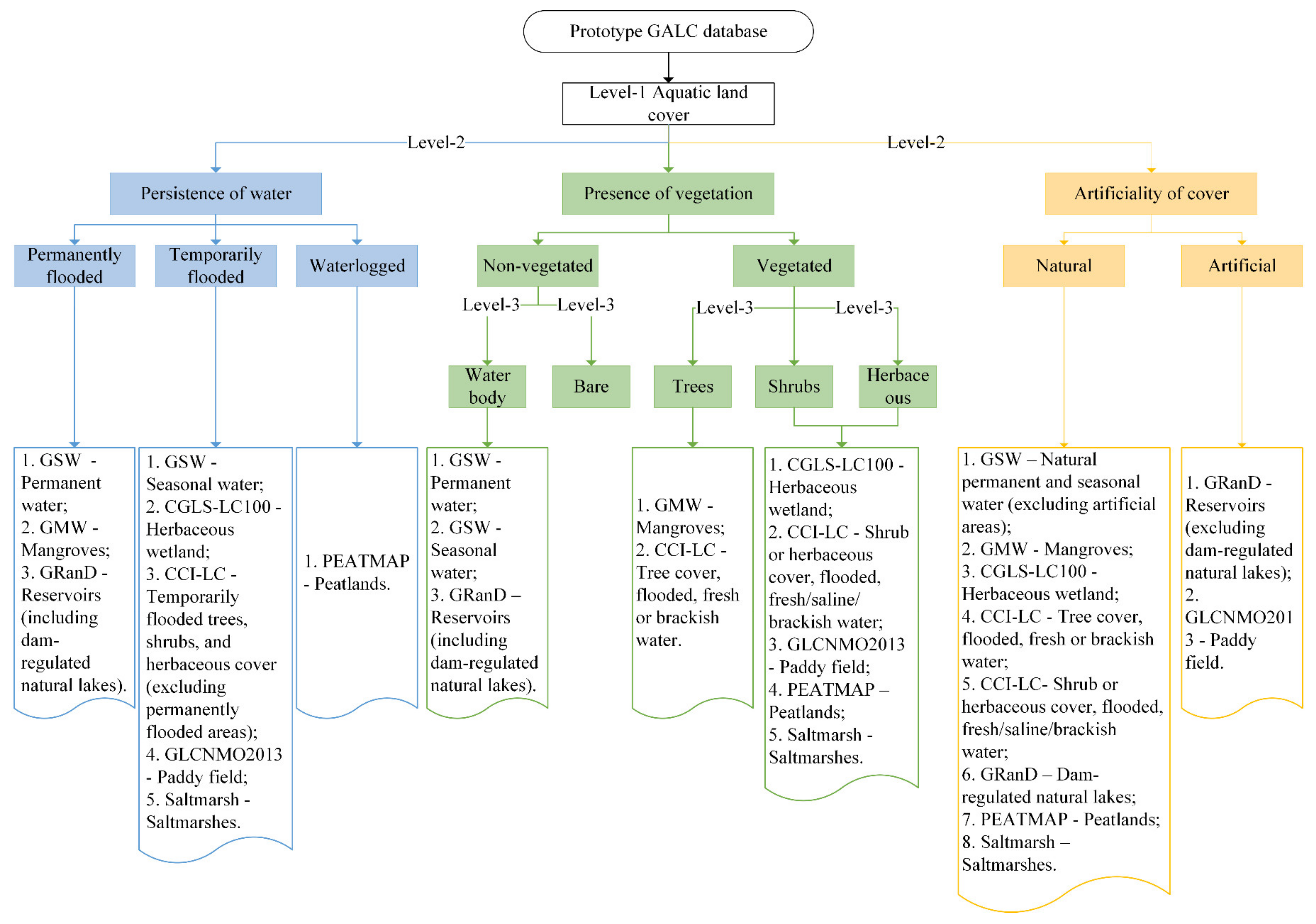
2.1. Global Aquatic Land Cover Characterization Framework

The prototype GALC database was built upon the LCCS-based GALC characterization framework proposed by Xu et al. [6] (Figure 2). Level-1 identifies aquatic land cover as a whole, representing the discrimination of aquatic and non-aquatic lands. Xu et al. [6] proposed five classifiers at Level-2, while this study focused on three of them; the persistence of water—the duration of water covering the surface; the presence of vegetation—the existence or absence of vegetation; and the artificiality of cover—whether or not a land cover is managed by humans. At Level-3, the vegetated and non-vegetated types are specified into more detailed classes by the life form classifier. This unique design was intended to enable users to generate maps according to their own needs.

2.1.1. Input Datasets

Input datasets were selected from the 33 GALC datasets reviewed by Xu et al. [6]. To ensure the thematic representativeness and quality of the input datasets, four criteria were used in the selection:
  • Thematic detail: The dataset should include at least one classifier of information at Level-2 or Level-3 of the reference GALC characterization framework.
  • Temporal range: To minimize the influence of land changes, the dataset should describe aquatic land cover within 2015 ± 3 years.
  • Spatial resolution: Considering the limited availability of high-resolution (≤100 m) datasets, the spatial resolution of the dataset should at least be ≤1 km.
  • Accuracy: The dataset should at least have an overall accuracy > 70% or being extensively evaluated (for those without quantitative assessment).
Finally, eight datasets (Table 1) meeting the above criteria were selected, of which five have a single aquatic class and three are GLC products. It should be noted that the selected datasets are considered the best to represent currently available datasets around 2015, however they might still be inferior compared with recently developed ones. If needed, users can include more advanced datasets to update the database.

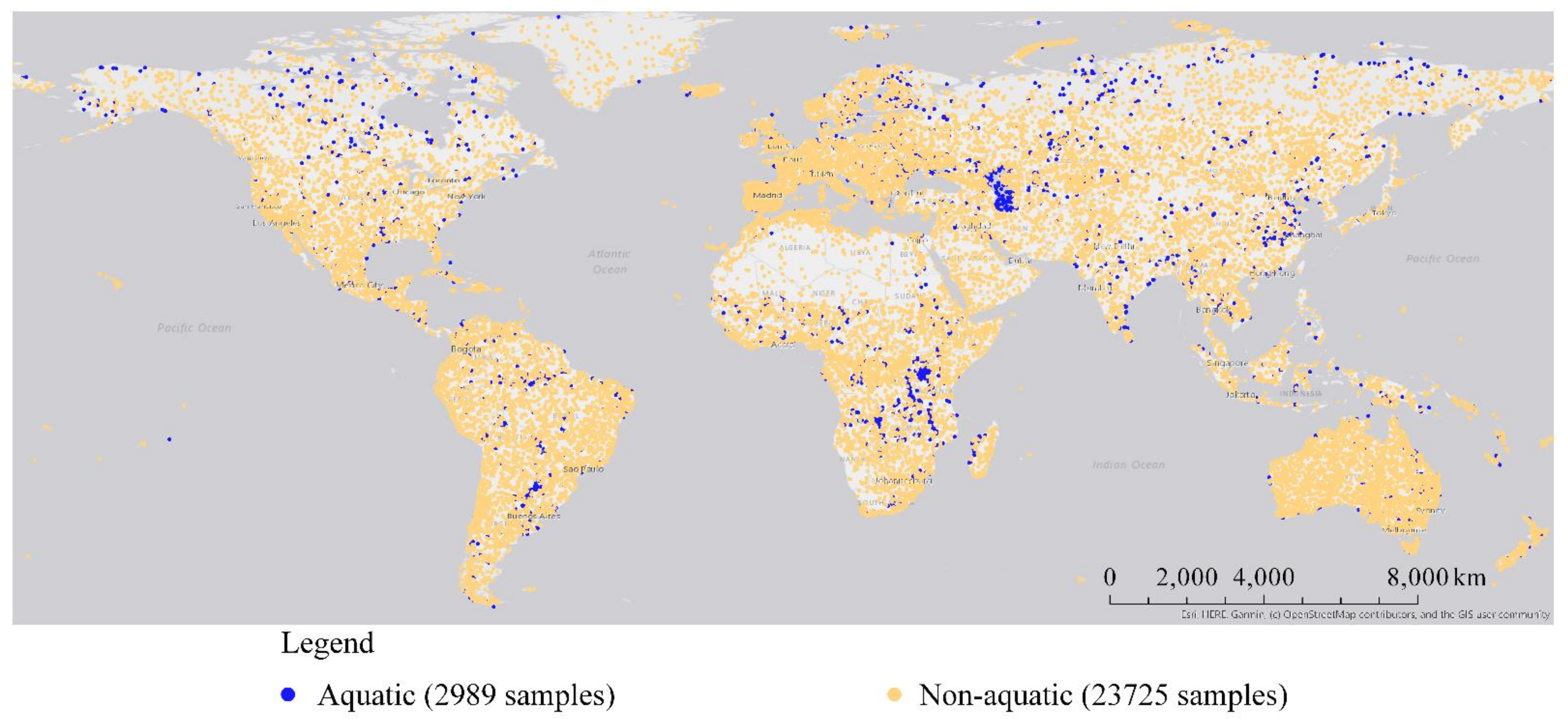
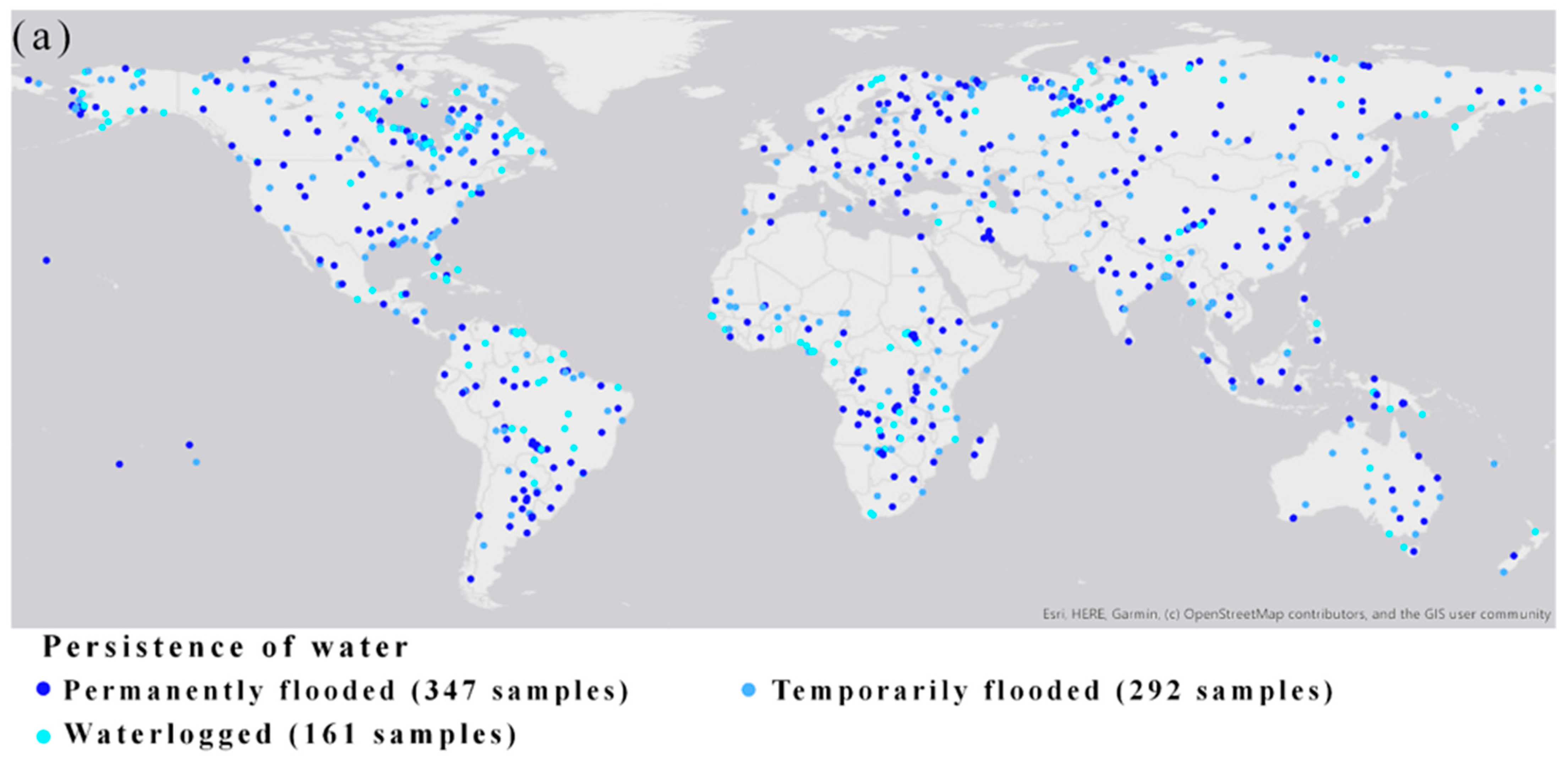
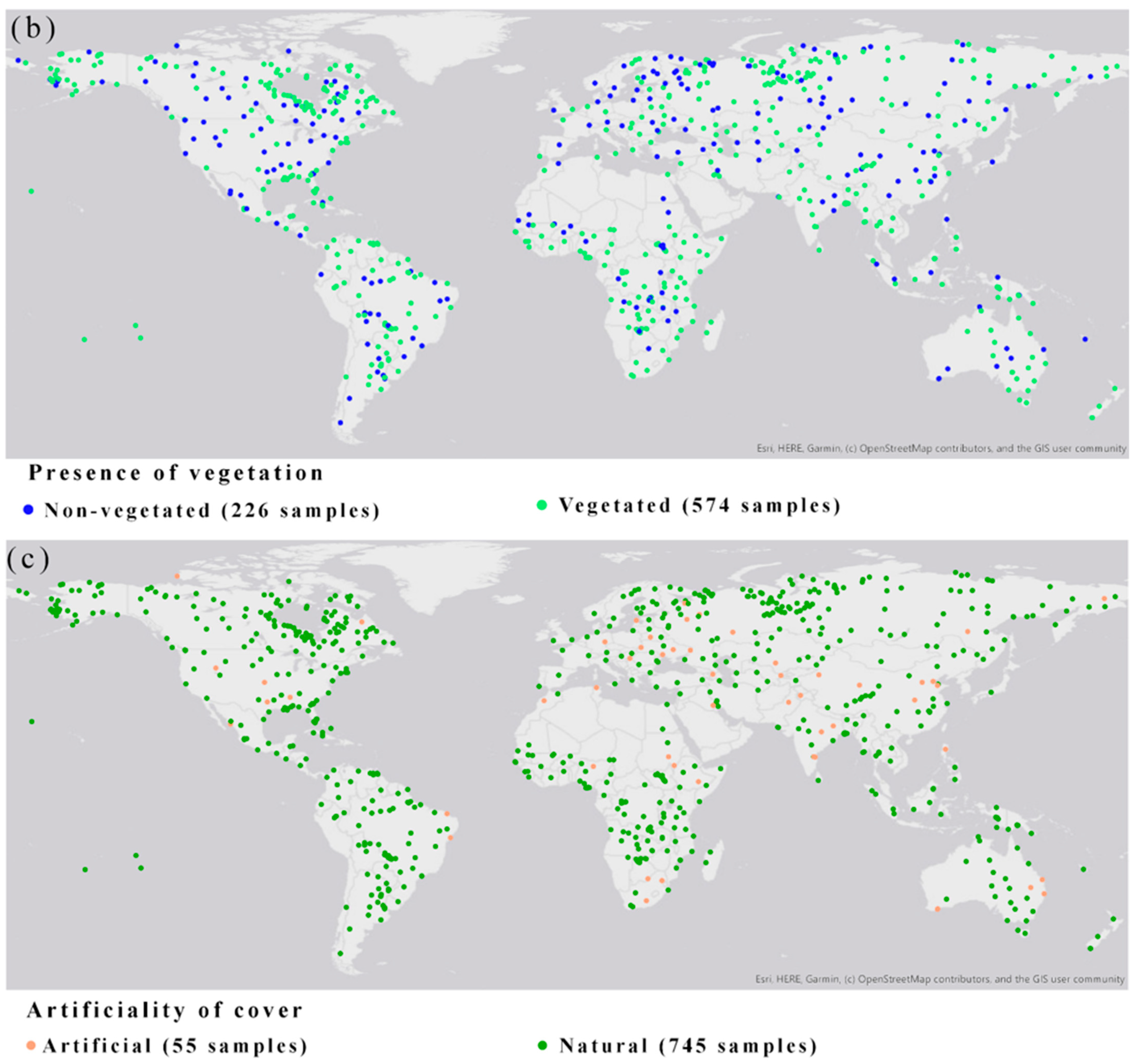
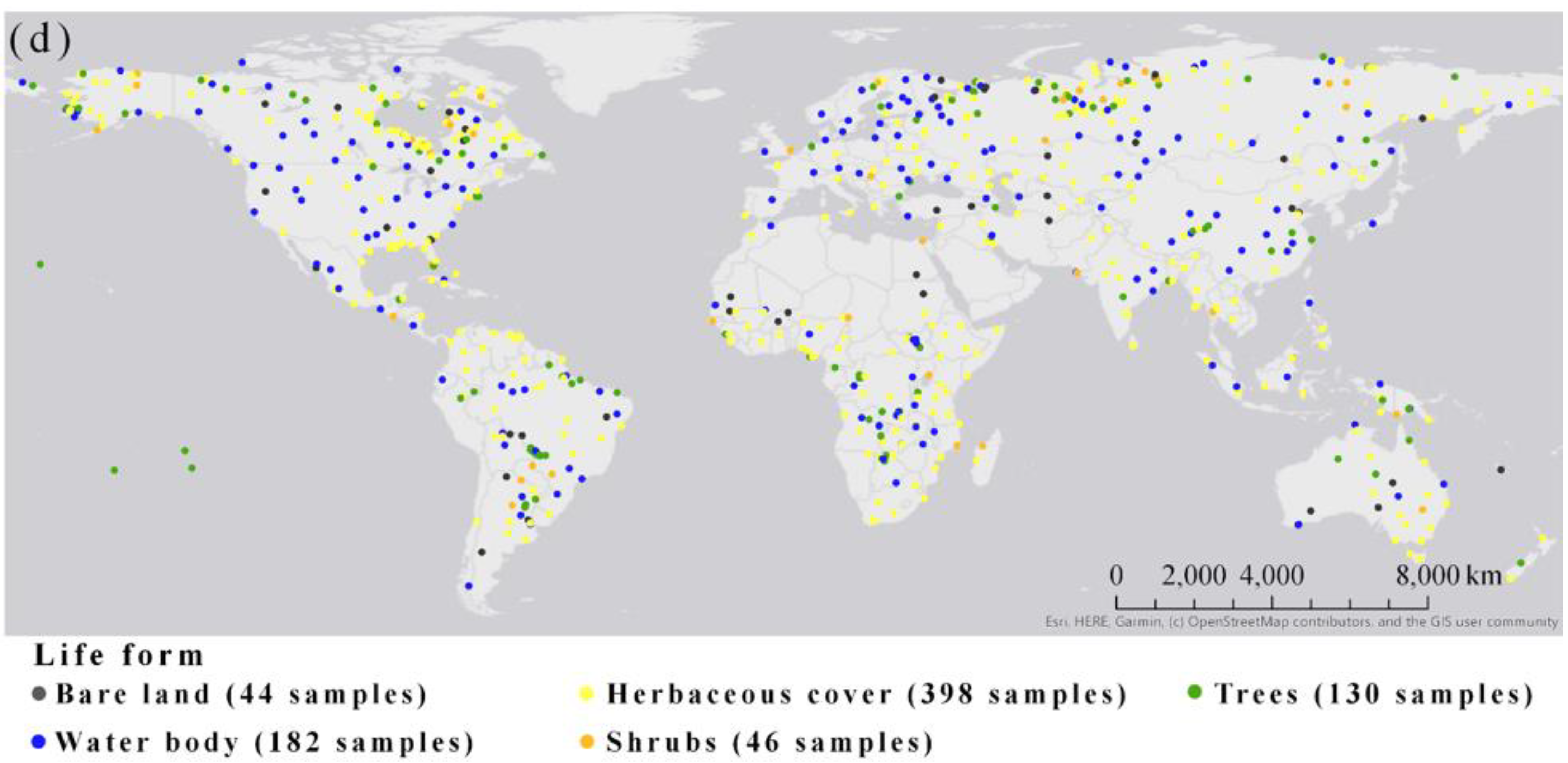
2.1.2. Validation Datasets

The Level-1 validation dataset used for accuracy assessment was collected as part of the CGLS-LC100 project [26]. The data include 26,714 sample sites across the globe (Figure 3), of which 2989 are aquatic and 23,725 are non-aquatic. Each sample site corresponds to a 100 m × 100 m pixel, and it is then divided into 100 subpixels at 10 m × 10 m resolution. The reference land cover was labelled at the subpixel level by a group of experts that were trained on separating different land cover types. In this study, the dominant type of the 100 subpixels was used to represent the land cover class of each 100 m × 100 m sample site. This dataset was generated following the stratified random sampling, and the inclusion probabilities of different sampling stratums were considered (see Tsendbazar et al. [27] for more details). The satellite imagery used for interpretation was from the year 2015.
The validation of Level-2 and Level-3 maps requires information on water persistence, vegetation presence, artificiality of cover, and life form types. Such detailed information was not recorded in the CGLS validation dataset. Thus, we randomly selected (i.e., simple random sampling) 800 aquatic sample sites (Figure 4) and visually interpreted the four classifiers on the Geo-wiki platform (http://www.geo-wiki.org, accessed 1 July 2009) using high-resolution Google Earth images, Bing maps, ESRI-WORLD imagery, and Sentinel-2 images from 2015. Time series of Sentinel-2 images (2015–2019) and the Normalized Difference Vegetation Index based on MODIS, Landsat, and PROBA-V were also used to characterize the information on the four classifiers.

2.2. Methods

2.2.1. Dataset Pre-Processing

The input datasets were reprojected onto the World Geodetic System (WGS) 1984 latitude/longitude and resampled into a spatial resolution of 0.00099° (approximately 100 m at the equator). Datasets in a vector format (i.e., GRanD, PEATMAP, global saltmarsh, GMW) were rasterized into the same projection and spatial resolution.
Among the input datasets, there exist some repeated classes (e.g., water bodies, mangroves) and overlapping areas, which may cause inconsistencies in the map integration process. To deal with this issue, the priority of each input dataset was evaluated using a ranking based on spatial resolution, temporal range, and accuracy. The general rule is that a dataset with a higher resolution, higher classification accuracy, and closer to the year 2015 was ranked higher. For datasets in a vector format, the larger range of the MMUs (Table 1) was taken as the spatial resolution. Furthermore, to facilitate the comparison of datasets with a differing spatial resolution, we divided the resolution into 6 groups, being ≤30 m, 30~100 m, 100~300 m, 300~500 m, 500~1000 m, and >1000 m. Datasets with a spatial resolution ≤ 30 m were ranked on top. For those datasets with a long time span (e.g., 1990–2013), the earlier starting year was used to rank that dataset. Regarding the accuracy ranking, the F-score [28] was calculated based on Equation (1) whenever the producer’s (PA) and user’s (UA) accuracies were available. For those without a quantitative accuracy assessment, the F-score was set to 0.
F s c o r e = 2 × U A × P A U A + P A ,
Based on the above rules, the three quality indicators of each dataset were given a ranking score (Table 2). The priority of the input datasets was determined using the average of the three rankings. Among the eight input datasets, GSW was ranked on top, followed by the GMW dataset. According to the ranking, water bodies from the CGLS-LC100, CCI-LC, and GLCNMO2013 dataset were excluded, and mangroves from GLCNMO2013 and the “tree cover, flooded, saline water” from CCI-LC were not used.

2.2.2. Legend Harmonization of Input Datasets

The legend harmonization was accommodating the legend of input datasets into “classifiers” of the reference GALC characterization framework based on the original class definition in the reference papers (Table 1). Take mangroves of the GMW dataset as an example, they are defined as “forested wetlands that are uniquely adapted to the intertidal zone” [18]. Accordingly, mangroves were translated as “aquatic” at Level-1, “permanently flooded” (as water is regularly available with tides in the intertidal zone throughout a year), “vegetated” (i.e., “forested wetland”), and “natural” (as the mangrove ecosystem is naturally formed) at Level-2, and “trees” at Level-3. There are also ambiguities or inconsistencies in class definitions identified in the harmonization process, and the following explains how we dealt with these issues.
  • Classes without information on the duration of water (e.g., herbaceous wetland of CGLS-LC100) were assumed as “temporarily flooded”.
  • Inconsistent class definition, i.e., the permanent water and seasonal water of the GSW dataset (Table 1), was adjusted to conform with the reference framework.
  • For classes including more than one cover type under the same classifier and making no distinction between them, several types were put under the same classifier, e.g., the life form type of PEATMAP included both herbaceous cover and shrubs (Table 3), as marshes and shrub swamps were both mapped by PEATMAP.

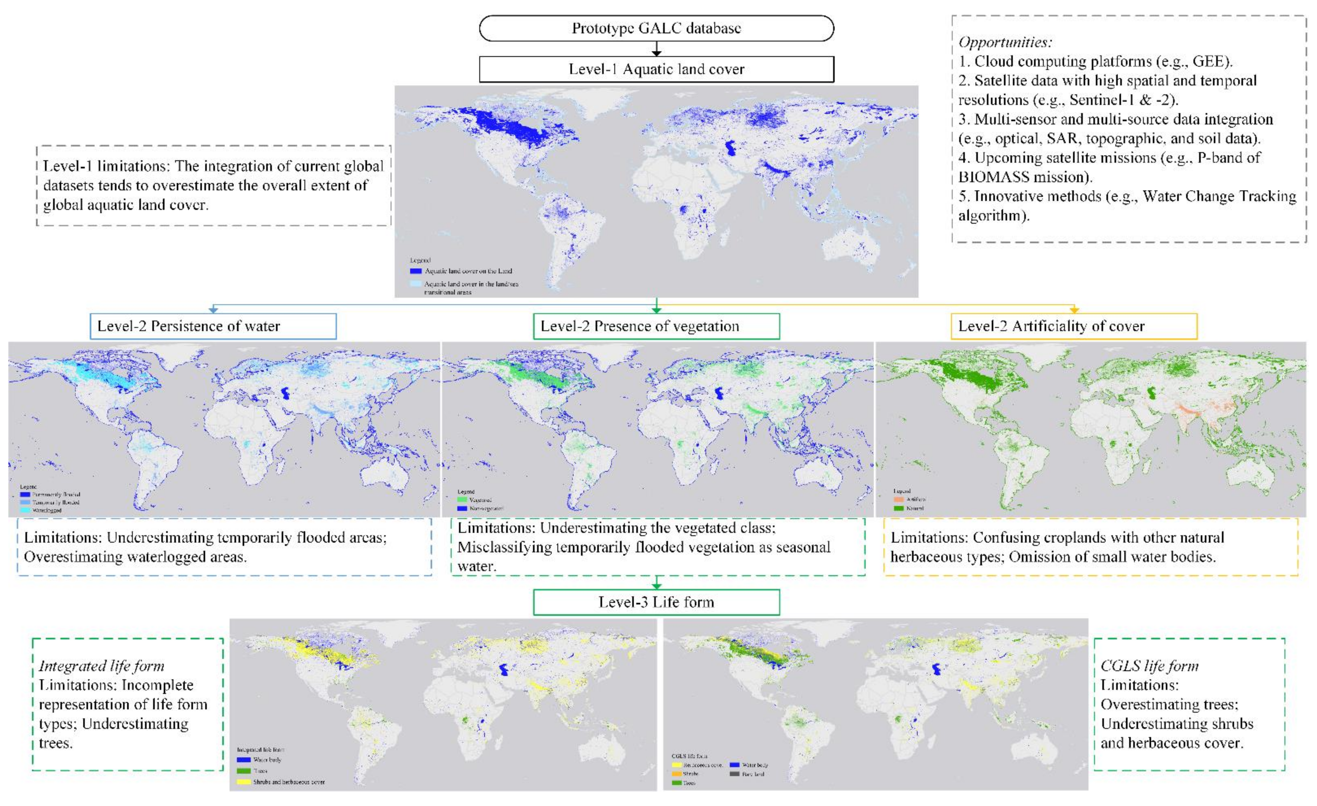
2.2.3. Generation of the Level-1, Level-2, and Level-3 Maps

Datasets were composited in the order of their priority rankings (Table 2) using the Geospatial Data Abstraction Library (GDAL) [29]. Specific GDAL commands used in the map generation were listed in Table S1 (Supplementary Materials). The integrated maps were converted to the world cylindrical equal area projection [30] to calculate the area of different classes.

Level-1: The Aquatic Land Cover Map

The Level-1 map (hereafter referred to as the “integrated Level-1 map”) was generated by combining the eight input datasets into one map. To get an insight on how many aquatic areas are on the land, the CGLS-LC100 land/sea mask [31] was applied to separate the aquatic land cover in the land/sea transitional zones and that on the land. The land area defined by the CGLS-LC100 land/sea mask is approximately 134.59 million km2 (excluding Antarctica and the land/sea transitional area).

Level-2: The Persistence of Water, Presence of Vegetation, and Artificiality of Cover Map

The Level-2 maps were created by combining corresponding classes (Table 3) into the three classifiers: persistence of water, presence of vegetation, and artificiality of cover. Figure 5 shows the input datasets to each classifier.
Prior to creating the persistence of water map, some processing was made to the input datasets. Firstly, the GSW water seasonality map was reclassified to generate the permanent water (≥9 months) and seasonal water (<9 months). Secondly, as the CCI-LC dataset mixed up the three water persistence types (Table 3), two masks were used to remove the permanently flooded area and the waterlogged area to get the “temporarily flooded trees, shrubs, and herbaceous cover”. The mask of permanently flooded areas was formulated by the three permanently flooded classes including mangroves of the GMW dataset, reservoirs of the GRanD dataset, and the permanent water from GSW. The PEATMAP was used to remove waterlogged areas from CCI-LC.
The GRanD dataset and the GSW dataset were also processed before generating the artificiality of cover map. The GRanD dataset contains natural lakes that are regulated by dams, which is not consistent with the LCCS-based definition because these lakes are naturally formed and do not require human maintenance over the long term. Therefore, we used the “natural lakes with regulation structure” from an external dataset called HydroLAKES [32] to separate natural lakes from reservoirs in the GRanD dataset. Likewise, the natural water and artificial water of the GSW dataset were separated using a mask formulated by the reservoirs (excluding dam-regulated natural lakes) from GRanD and the paddy field from GLCNMO2013.
The presence of vegetation map was composited from the Level-3 life form types (Figure 5) into the vegetated and non-vegetated categories.

Level-3: The Life Form Map

The Level-3 map was created by combining corresponding classes for the five life form types (Figure 2). As none of the selected input datasets contain aquatic classes of “bare land”, and additionally, shrubs and herbaceous cover cannot be separated in PEATMAP as well as CCI-LC (Table 3), the Level-3 map integrated by the eight input datasets (hereafter called the “integrated life form” map) comprised only three classes, including “water body”, “trees”, and “shrubs and herbaceous cover” (Figure 5).
To acquire a more complete delineation of the five life form types, another map (hereafter called the “CGLS life form”) was created using the Fractional Land Cover (FLC) maps of the CGLS-LC100 product [24]. This product comprises ten FLC maps, and the value of each map indicates the proportion of a 100 m × 100 m pixel filled with a specific land cover class. As several classes might coexist within the same pixel, we firstly generated a global dominant cover map using the ten maps in Google Earth Engine (GEE). Eight classes that correspond to our classification scheme, i.e., “bare/sparse vegetation”, “permanent water”, “seasonal water”, “herbaceous grassland”, “cropland”, “moss/lichen”, “shrubland”, and “tree” were then selected from the global dominant cover map and exported from GEE. The resulting map was finally restrained to aquatic areas using the integrated Level-1 map created in this study in GDAL.

2.2.4. Accuracy Assessment

The integrated Level-1 map was assessed using 26,714 samples from the Level-1 validation dataset (Figure 3). Accuracy estimates such as overall accuracies (OA), class accuracies, and their confidence intervals (CI, at 95% confidence level) were calculated using the same method described in Tsendbazar et al. [27] following the good practice recommendations of stratified random sampling suggested by Olofsson et al. [33]. The sample inclusion probabilities were used in the accuracy calculation to reduce bias arising from the sampling design.
The three Level-2 maps and two Level-3 maps were assessed using the 800 sample sites shown in Figure 4. As some locations of this validation dataset had no data on the Level-2 or Level-3 maps, not all of the 800 samples were used in the confusion matrix calculation. The method of calculating the accuracy for simple random sampling [33,34] was implemented for the Level-2/3 maps. Accuracies were adjusted based on the sample-counted confusion matrix and area proportions of the mapped land cover classes. To compare the accuracy of the two Level-3 maps, herbaceous cover and shrubs on the CGLS life form map were merged and the bare land was excluded in the validation.

3. Results

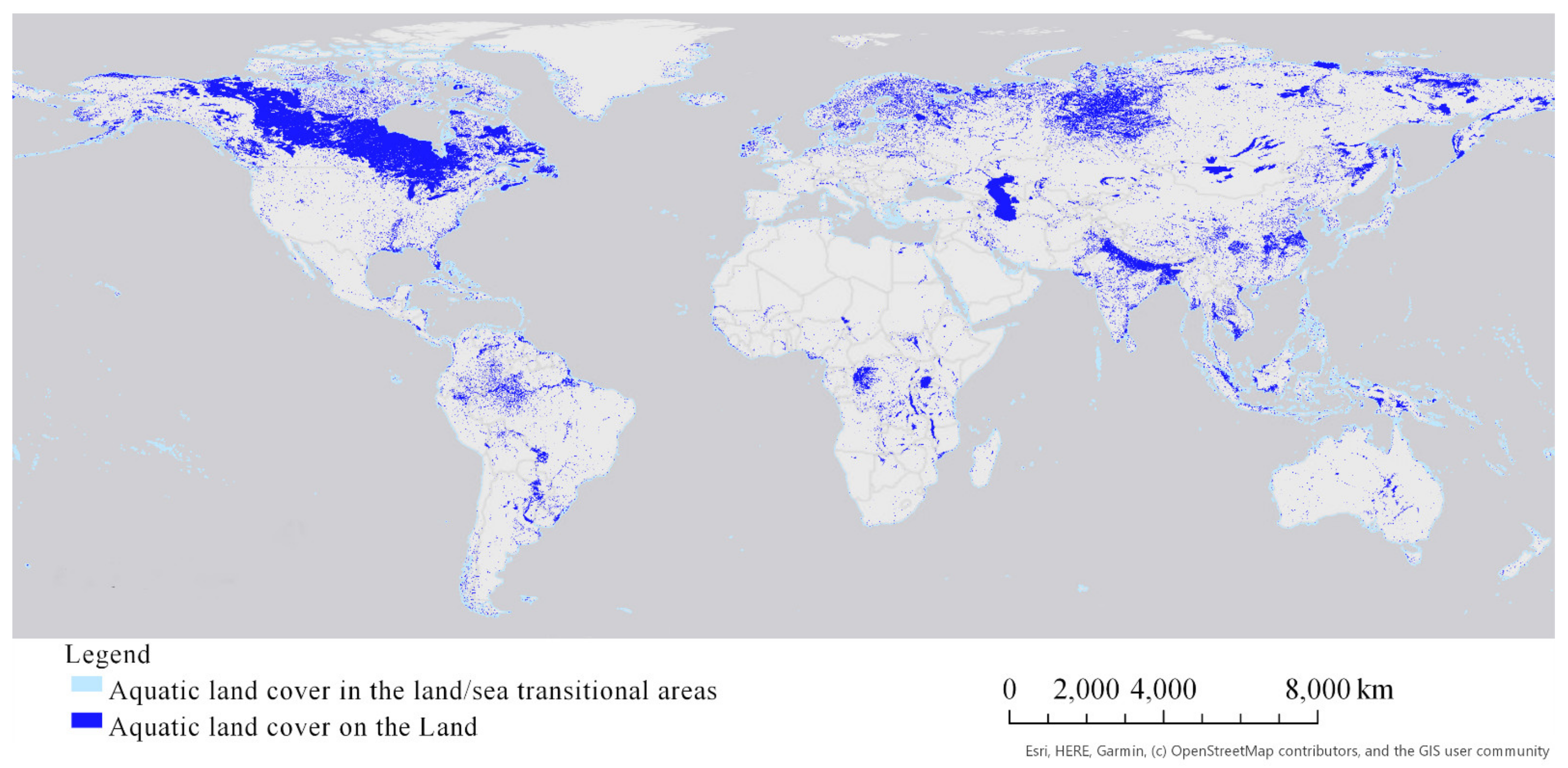
3.1. Level-1: Aquatic Land Cover

The integrated Level-1 map is presented in Figure 6. The total area of GALC is estimated as 27.5 million km2, of which 15.3 million km2 is on the land (i.e., 11.4% of the global land area). The confusion matrix correcting unequal inclusion probabilities is shown in Table 4. The count-based confusion matrix is provided in Table S2 (Supplementary Materials). Although the integrated Level-1 map achieved an overall accuracy of 93.0% ± 0.4% (at 95% CI, Table 4), it had considerable commission errors (100%—UA) in mapping aquatic land cover. It was observed that the area-weighted UA of aquatic lands (32.7%, Table 4) was much lower compared with that of the count-based confusion matrix (58.7%, Table S2). This could be explained by the fact that non-aquatic sample sites represent a much larger proportion of the Earth’s surface, therefore they carry larger weights when accounting for the unequal inclusion probabilities than aquatic sample sites. Still, even when the area weights of the classes were not considered, a lower UA of the aquatic class was notable.

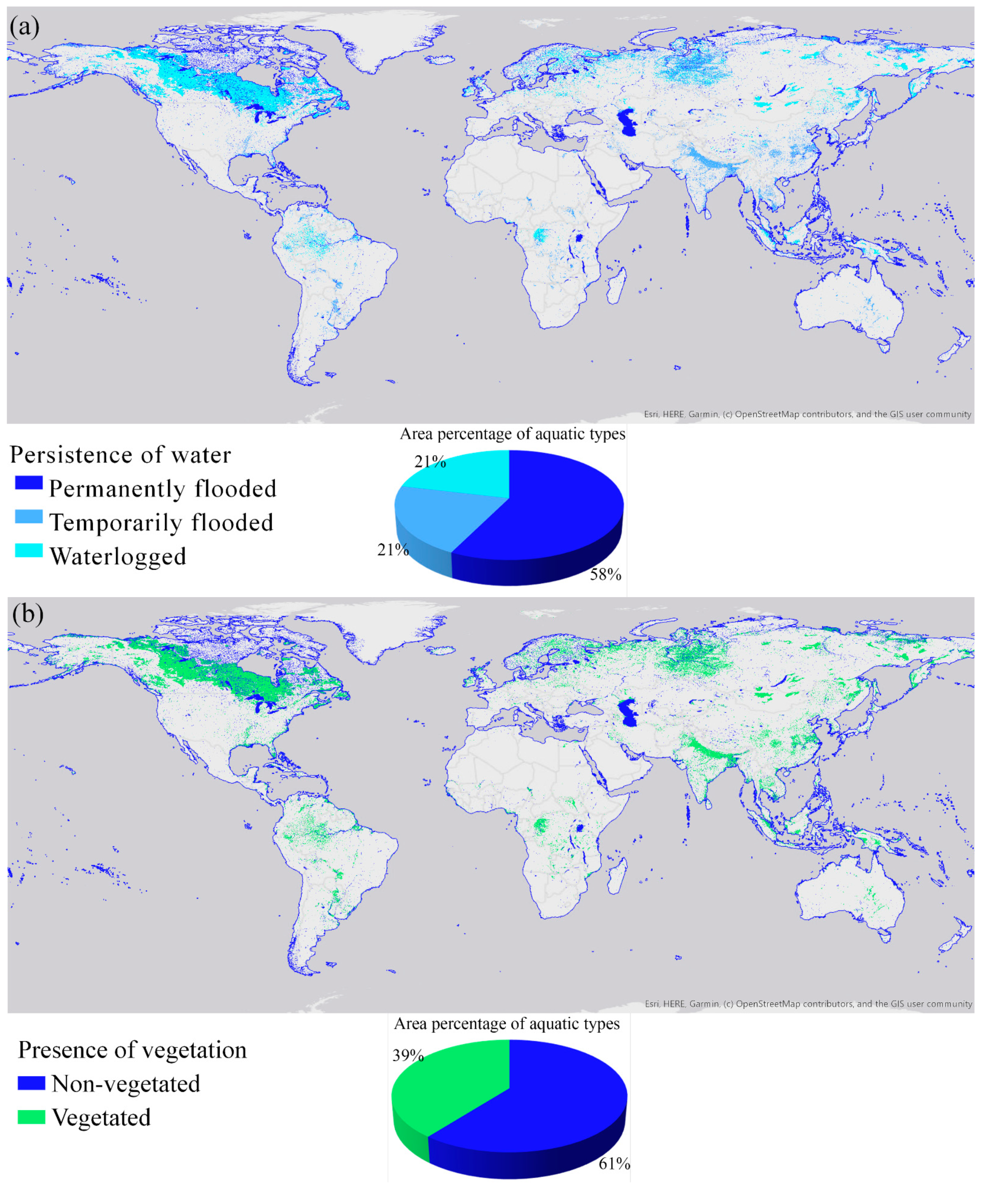
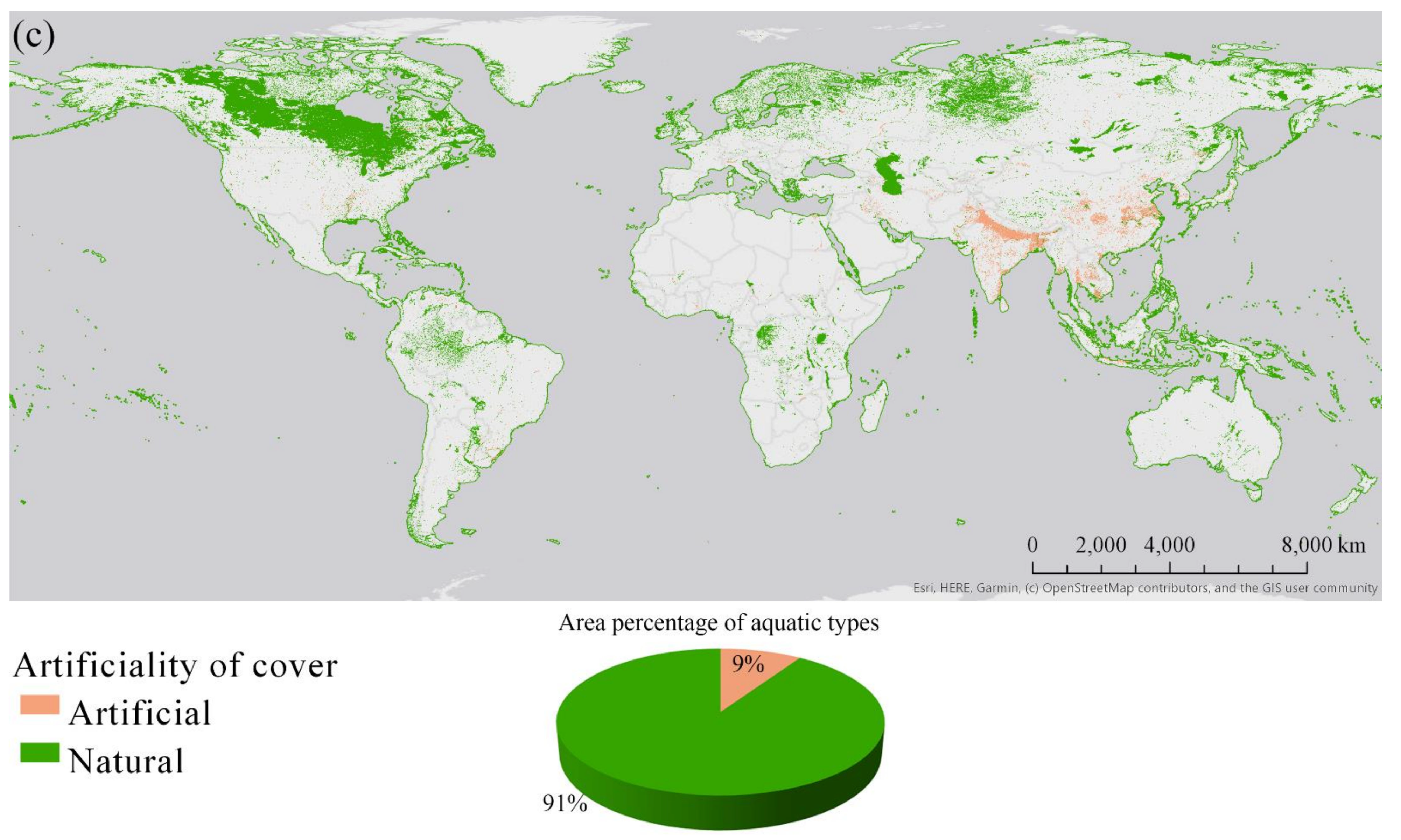
3.2. Level-2: Persistence of Water, Presence of Vegetation, and Artificiality of Cover

The Level-2 maps are presented in Figure 7. The area-weighted and count-based confusion matrices of the three maps are provided in Table 5, Table 6 and Table 7 and Tables S3–S5 (Supplementary Materials), respectively. According to the area statistics, the majority of global aquatic lands are permanently flooded (58%, Figure 7a), non-vegetated (61%, Figure 7b), and natural (91%, Figure 7c).
The overall accuracy of the persistence of water map was 50.7 ± 3.8% (at 95% CI, Table 5). This map achieved a higher UA and PA in permanently flooded areas than that of the temporarily flooded and waterlogged areas. The map overrepresented the waterlogged class at the cost of the temporarily flooded class. Almost 72% (100%—PA) of the reference temporarily flooded samples were misclassified as the waterlogged and permanently flooded types.
The presence of vegetation map achieved an overall accuracy of 63.5 ± 3.6% (at 95% CI, Table 6). Generally, the PA of the non-vegetated class was much higher than its UA, and a contrary situation occurred for the vegetated class, meaning that this map tended to overestimate the non-vegetated class while underestimating the vegetated class.
The natural aquatic class on the artificiality of cover map was highly accurate in terms of PA and UA (i.e., both exceeded 90%, Table 7). However, even though the overall accuracy (88.3 ± 2.0%) was high, artificial aquatic areas were poorly characterized by this map, with the UA and PA being only 26.8 and 37.1%, respectively.

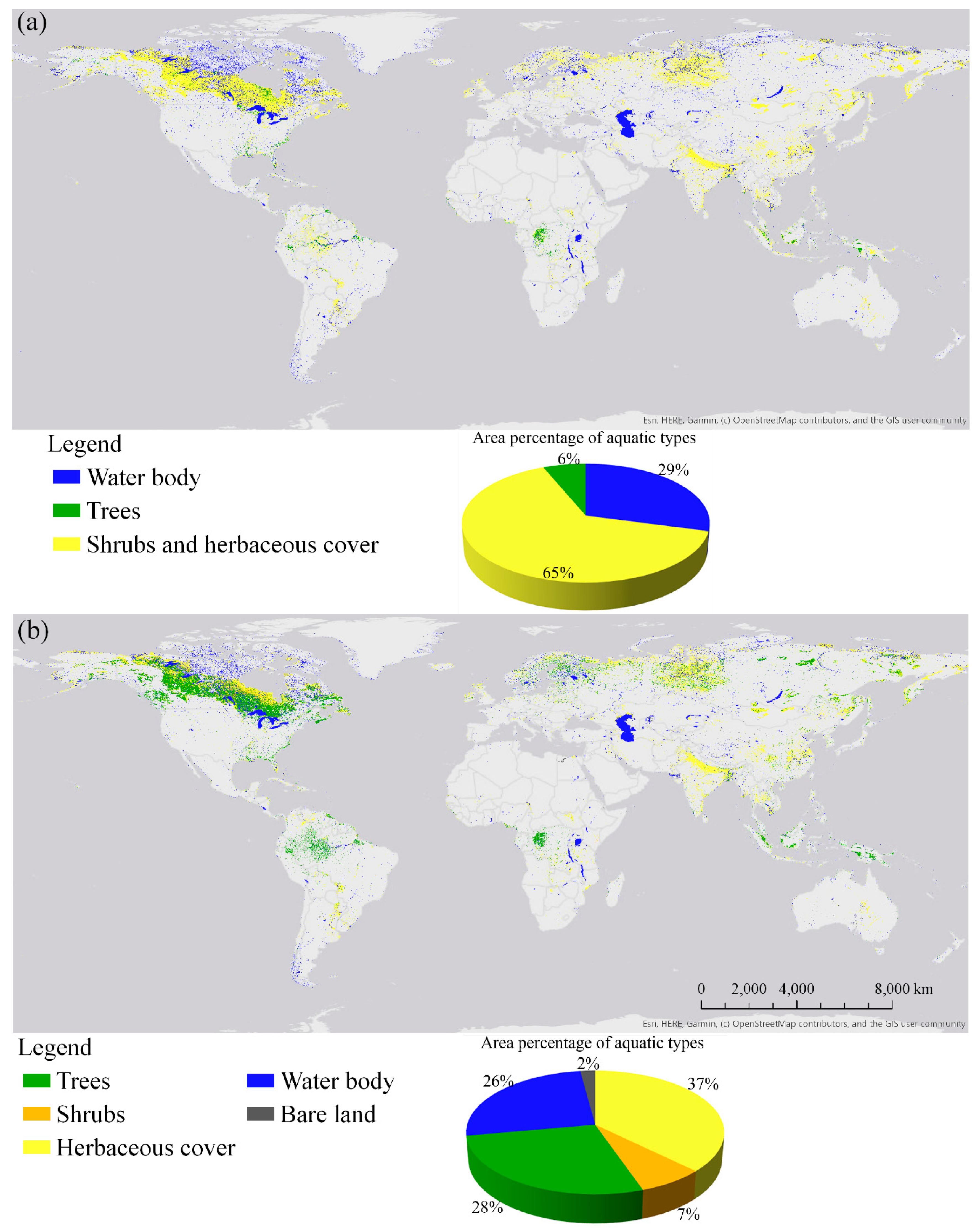
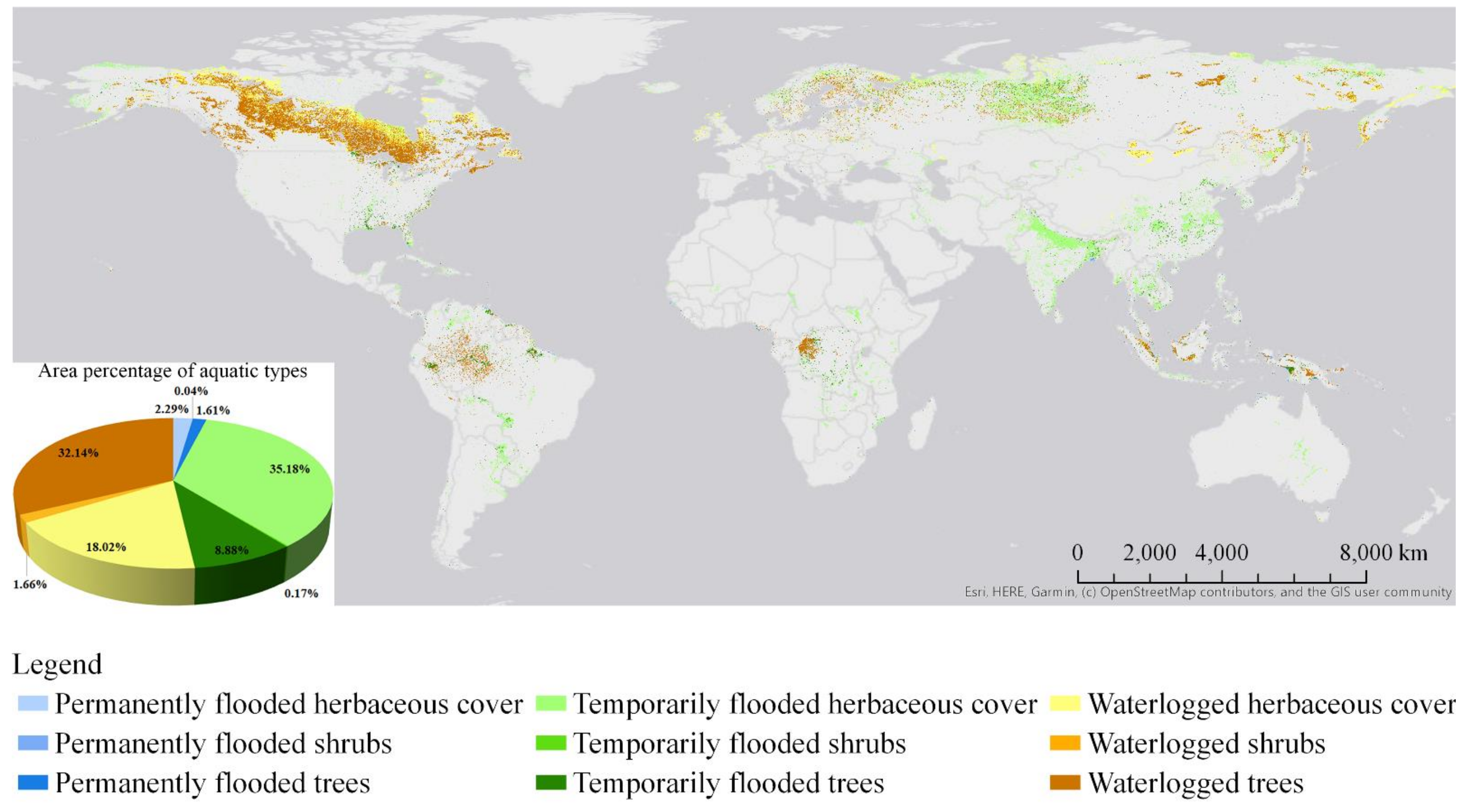
3.3. Level-3: Life Form

The integrated life form map and the CGLS life form map are shown in Figure 8. Their area-weighted and count-based confusion matrices are provided in Table 8 and Table S6 (Supplementary Materials), respectively. The two Level-3 maps had a similar spatial distribution and areal percentage of water bodies, while they differed a lot in other life form types (pie charts in Figure 8). The overall accuracies of both maps were relatively low (Table 8). The integrated life form map obtained a higher OA (56.9 ± 4.3%) than the CGLS life form map (50.0 ± 4.1%).
The integrated life form map was better at characterizing shrubs/herbaceous cover than the CGLS life form map (Table 8), while at the same time it underestimated trees with around 79% (calculated from Table 8) of the reference tree samples being omitted from shrubs/herbaceous cover. The CGLS life form map was better at characterizing trees than the integrated life form map, while it had a tendency of overestimating trees at the cost of shrubs/herbaceous cover.

4. Discussion

With the increasing demand for water resources, the characterization of aquatic land cover has attracted more and more attention. By reframing current datasets consistently, this research created a three-level prototype GALC database (Figure 9) and evaluated its performance rigorously. In this section, the limitations of existing datasets and possible reasons behind those limitations are discussed. The evolving EO opportunities to improve the GALC characterization are also highlighted. Although the prototype GALC database was developed and evaluated in a systematic way, findings in this study might be subject to some limitations because of the limited number of “waterlogged”, “artificial”, and “shrub” sample sites for a global assessment. These classes should be investigated further if sufficient validation data are available. Nevertheless, obtaining high-quality global aquatic reference datasets with detailed information on classifiers requires considerable time and expertise given the heterogeneous and dynamic characteristics of aquatic land cover.

4.1. Limitations of Current Global Datasets in GALC Mapping

4.1.1. General Classification of Global Aquatic Land Cover

The global aquatic area on the land estimated by the integrated Level-1 map is 15.3 million km2, with a tendency of overestimating the total extent of GALC (Table 4). The overestimation could have originated from the input datasets. For instance, the CGLS-LC100 product is prone to misclassify the herbaceous wetland with terrestrial grasslands in the land cover classification [26].
The most recent research on the mapping of the overall distribution of GALC made by Hu et al. [35] and Tootchi et al. [36] reported an estimate of 29.8 million km2 and 29 million km2 of aquatic area on the land, respectively. According to the result of our accuracy assessment, the two estimates could also be considerably overestimated, indicating a global product that can accurately separate the aquatic from the non-aquatic land is still needed. Considering the key components of aquatic ecosystems, it is more difficult to map aquatic vegetation and wet soils remotely than water bodies [37]. However, integrating multi-source data such as optical, Synthetic Aperture Radar (SAR), soil, and topographic features has been demonstrated useful in improving the general-level classification of aquatic lands [38].

4.1.2. Classification of Persistence of Water, Presence of Vegetation, and Artificiality of Cover

The validation of the persistence of water map highlights that current datasets have limitations of characterizing the waterlogged and temporally dynamic types (Table 5). One of the reasons is that the classification of waterlogged areas without evident surface flooding is more difficult than detecting open surface water because the contrast between wet soils and their surroundings is less pronounced [39]. In addition, the input datasets used to generate the temporarily flooded class represent mainly vegetated aquatic types (Figure 5), while characterizing water bodies under vegetation has always been challenging [4]. Furthermore, the information on water persistence is still lacking among existing datasets. Except for the GSW dataset that characterizes the water seasonality, other input datasets were all static maps missing the information on water duration.
The presence of vegetation map tends to underestimate vegetated aquatic lands (Table 6). The main cause lies in that identifying vegetated aquatic land cover globally remains challenging based on remote sensing classification [27]. Unlike open surface water, vegetated aquatic lands are complicated by their distribution throughout tropical to boreal environments that encompass a wide variety of vegetation types, hydrological regimes, and land-use impacts [37]. Another possible cause could be the inconsistent definition of the input datasets with our reference classification framework. For example, the GSW dataset, which was used as an input of the “non-vegetated” class in this study, considers vegetated areas that represent short-duration flooding events as seasonal water bodies [19].
The artificiality of cover map performs well in characterizing natural aquatic lands (Table 7), while defects of the two source datasets (i.e., GLCNMO2013 and GRanD) lead to low accuracies of the artificial class. Firstly, as a main source providing the information on aquatic croplands, GLC products often confuse croplands with other natural herbaceous types [25]. Secondly, the GRanD dataset delineated reservoirs with a storage capacity of >0.1 km3 while excluding smaller reservoirs, which might cause the omission of artificial water bodies, such as fishponds.

4.1.3. Classification of Aquatic Life Forms

As an extension of the Level-2 presence of vegetation map, the lower overall accuracy of the Level-3 life form map (Table 8) demonstrates prominent gaps existing in the characterization of the vegetation presence and detailed vegetation types in aquatic areas. The significant underestimation of trees on the integrated life form map indicates that the two source input datasets, i.e., GMW and CCI-LC, also omitted considerable trees under an aquatic environment globally. Both the integrated life form map and the CGLS life form map have the issue of misclassifying trees, shrubs, and herbaceous cover. In fact, these types are indeed challenging to be separated solely by optical sensors as they have similar spectral signals [26]. Moreover, shrubs always grow with herbaceous vegetation or trees, making it difficult to be mapped independently.
The CGLS-LC100 FLC maps, offering the proportional estimates for basic land cover types, allow users to tailor the maps to their own applications. However, the life form map derived from these maps does not perform well in aquatic areas (Table 8), even though it has been reported with higher accuracies in the global validation [26]. The poor prediction could have resulted from the seasonal or even daily water dynamics which make it challenging to estimate the exact fraction of different land cover types [37].

4.2. Evolving EO Opportunities to Improve the GALC Characterization

Recent developments of cloud-based computational platforms, such as Google Earth Engine [40], offer a unique opportunity for global aquatic land cover mapping with its free access to tremendous volumes of EO data [41]. The Sentinel satellite imagery provided by the European Space Agency’s Copernicus programme can be easily accessed on the GEE platform. Data acquired from the Sentinel-1 and Sentinel-2 satellites have a spatial resolution up to 10 m and temporal resolution reaching six days and five days, respectively. The improved spatial and temporal resolutions allow capturing the variations of water occurrence [42] and small water bodies [43]. The three red-edge bands and two shortwave infrared (SWIR) bands of Sentinel-2 imagery are valuable in discriminating spectrally similar vegetation types [44]. The SWIR bands sensitive to both soil and vegetation moisture could contribute to characterizing waterlogged areas [45]. The Sentinel-1 C-band SAR data has been successfully used to identify water under temporarily flooded vegetation [46].
Integrating multi-sensor (e.g., Landsat and Sentinel-2) and multi-source data (e.g., optical, radar, topographic, and soil data) has a better capacity to capture the inundation extent, vegetation structure, and hydroperiod variations [38] and thus is more suitable to discriminate between the aquatic and terrestrial uplands as well as the temporally dynamic and complex aquatic types (e.g., Level-3 classes). Some new datasets also have potential in improving the GALC characterization. For example, incorporating the height information, such as the recent global forest canopy height dataset [47], could reduce confusions of trees and shrubs.
SAR data at longer wavelengths can penetrate tree canopies, and specifically the P-band SAR from the upcoming BIOMASS mission [48] has higher chances to reach the surface underneath [49]. Such a design would enable characterizing the water under dense vegetation canopies and improving the mapping of vegetation in aquatic environments and water persistence in densely vegetated areas. Many innovative methods for aquatic land mapping have also been proposed that are suited to multi-temporal images, such as the Water Wetness Presence Index [39] and the Water Change Tracking algorithm [50]. Evaluating these methods is beyond the scope of the current paper.

4.3. Potential of the Prototype GALC Database in Addressing Multiple User Needs

Regardless of the accuracy of integrated maps, the developed prototype database showed what a comprehensive and user-oriented GALC product could comprise. With sufficient flexibility, the prototype database allows users to obtain their required information by combining maps at various levels and classifiers. As mentioned before, climate modelers may require a map showing the vegetation type under different water persistence for accurate estimation of methane emissions. Such a map (Figure 10) could be generated by combining the Level-2 persistence of water map with the vegetation types from the Level-3 CGLS life form map.
The prototype database also has important implications for aquatic ecosystem management. Firstly, the GALC maps could serve as basic inputs to hydrological and hydrodynamic models [51]. Secondly, these maps are helpful for the determination of appropriate input parameters for hydrological modeling. For example, in flood risk management, roughness estimation is an important step to simulate flood flows using hydrological models [52]. The roughness is strongly influenced by the physical properties of surface materials, such as the vegetation density, which differ among vegetation types. In this sense, accurate characterization of the Level-2 (i.e., presence of vegetation, the artificiality of cover) and Level-3 maps hold considerable potential in improving the accuracy of roughness estimation, which can be beneficial for mitigating flood risks and conserving aquatic ecosystems.
Maps in the GALC database can also be integrated with external datasets. One of the important applications is for global land change monitoring. For instance, integrating the Level-1 map with land/vegetation change datasets (e.g., the Global Forest Watch datasets [53]) or combining the Level-2 and Level-3 maps with water change products (e.g., [54]) allows for monitoring changes in aquatic areas. Such information is valuable for evaluating land disturbance and vegetation regeneration dynamics in aquatic ecosystems.
The evolving EO opportunities provided for more accurate and continuous GALC mapping enables updating and enriching the database routinely (e.g., annually). The Sustainable Development Goal 6 [55] has put an emphasis on protecting and restoring water-related ecosystems. A comprehensive and continuous GALC database would contribute to the implementation of this goal.

5. Conclusions

With the aim of assessing the integration of current global datasets for comprehensive and user-oriented GALC mapping, this study has created a prototype database for 2015 which includes six maps at three levels with 100 m resolution. The combination of existing datasets tends to overestimate the general extent of aquatic land cover. At Level-2, the persistence of water map is good at characterizing permanently flooded areas, while weak in waterlogged areas without evident surface flooding and temporarily flooded areas with greater water variations—the presence of vegetation map tends to underestimate the vegetated aquatic land cover while overestimating the non-vegetated ones; natural aquatic types are sufficiently mapped while artificial aquatic lands (i.e., reservoirs and paddy fields) are poorly represented. Current datasets cannot accurately characterize the detailed life form types (Level-3) such as trees and shrubs for aquatic land cover. Although the integrated maps have relatively low accuracies, the prototype GALC database is flexible for deriving multiple user-required maps and has important implications for aquatic ecosystem management and land change monitoring in aquatic areas. The availability and easier access of high spatial and temporal resolution data and the development of new satellite missions and aquatic land cover classification methods provide opportunities to address the limitations in current GALC characterization. This work provides insights for the next-generation GALC mapping and helps future map users as well as producers to avoid some of the limitations of current global datasets.

Supplementary Materials

The following are available online at https://www.mdpi.com/article/10.3390/rs13194012/s1, Table S1: GDAL commands used in the map generation, Table S2: Count-based confusion matrix for the integrated Level-1 map, Table S3: Count-based confusion matrix for the Level-2 persistence of water map, Table S4: Count-based confusion matrix for the Level-2 presence of vegetation map, Table S5: Count-based confusion matrix for the Level-2 artificiality of cover map, Table S6: Count-based confusion matrix for the Level-3 maps.

Author Contributions

Conceptualization, P.X., N.-E.T., M.H. and J.G.P.W.C.; formal analysis, P.X.; methodology, P.X. and N.-E.T.; supervision, M.H. and J.G.P.W.C.; writing—original draft preparation, P.X.; writing—review and editing, P.X., N.-E.T., M.H. and J.G.P.W.C. All authors have read and agreed to the published version of the manuscript.

Funding

This research received no external funding.

Data Availability Statement

The datasets used in this study are available from online repositories, with access links provided in Table 1. The maps produced in this study can be accessed from https://figshare.com/s/e06ad06fdc79e4aa43de. (accessed on 2 September 2021).

Acknowledgments

This project is funded by the China Scholarship Council (NO. 201804910841).

Conflicts of Interest

The authors declare no conflict of interest.

References

  1. Di Gregorio, A. Land Cover Classification System: Classification Concepts and User Manual; Food and Agriculture Organization: Rome, Italy, 2005. [Google Scholar]
  2. Mitsch, W.J.; Gosselink, J.G. Wetlands, 4th ed.; Wiley: New York, NY, USA, 2007. [Google Scholar]
  3. Finlayson, C.M.; Gardner, R.C. Ten key issues from the Global Wetland Outlook for decision makers. Mar. Freshw. Res. 2021, 72, 301–310. [Google Scholar] [CrossRef]
  4. Slagter, B.; Tsendbazar, N.-E.; Vollrath, A.; Reiche, J. Mapping wetland characteristics using temporally dense Sentinel-1 and Sentinel-2 data: A case study in the St. Lucia wetlands, South Africa. Int. J. Appl. Earth Obs. Geoinf. 2020, 86, 102009. [Google Scholar] [CrossRef]
  5. Hu, S.; Niu, Z.; Chen, Y. Global Wetland Datasets: A Review. Wetlands 2017, 37, 807–817. [Google Scholar] [CrossRef]
  6. Xu, P.; Herold, M.; Tsendbazar, N.-E.; Clevers, J.G.P.W. Towards a comprehensive and consistent global aquatic land cover characterization framework addressing multiple user needs. Remote Sens. Environ. 2020, 250, 112034. [Google Scholar] [CrossRef]
  7. Lehner, B.; Döll, P. Development and validation of a global database of lakes, reservoirs and wetlands. J. Hydrol. 2004, 296, 1–22. [Google Scholar] [CrossRef]
  8. Amler, E.; Schmidt, M.; Menz, G. Definitions and Mapping of East African Wetlands: A Review. Remote Sens. 2015, 7, 5256–5282. [Google Scholar] [CrossRef] [Green Version]
  9. Zhang, B.; Tian, H.; Lu, C.; Chen, G.; Pan, S.; Anderson, C.; Poulter, B. Methane emissions from global wetlands: An assessment of the uncertainty associated with various wetland extent data sets. Atmos. Environ. 2017, 165, 310–321. [Google Scholar] [CrossRef]
  10. Hondula, K.L.; Jones, C.N.; Palmer, M. Effects of seasonal inundation on methane fluxes from forested freshwater wetlands. Environ. Res. Lett. 2021, 16, 084016. [Google Scholar] [CrossRef]
  11. Turetsky, M.R.; Kotowska, A.; Bubier, J.; Dise, N.B.; Crill, P.; Hornibrook, E.R.C.; Minkkinen, K.; Moore, T.R.; Myers-Smith, I.H.; Nykänen, H.; et al. A synthesis of methane emissions from 71 northern, temperate, and subtropical wetlands. Glob. Chang. Biol. 2014, 20, 2183–2197. [Google Scholar] [CrossRef]
  12. Ramsar Convention Secretariat. An Introduction to the Convention on Wetlands (Previously the Ramsar Convention Manual); Ramsar Convention Secretariat: Gland, Switzerland, 2016. [Google Scholar]
  13. Warner, B.G.; Rubec, C.D.A. The Canadian Wetland Classification System; Wetlands Research Centre, University of Waterloo: Waterloo, ON, Canada, 1997. [Google Scholar]
  14. Herold, M.; Mayaux, P.; Woodcock, C.E.; Baccini, A.; Schmullius, C. Some challenges in global land cover mapping: An assessment of agreement and accuracy in existing 1 km datasets. Remote Sens. Environ. 2008, 112, 2538–2556. [Google Scholar] [CrossRef]
  15. Tsendbazar, N.-E.; de Bruin, S.; Herold, M. Integrating global land cover datasets for deriving user-specific maps. Int. J. Digit. Earth 2017, 10, 219–237. [Google Scholar] [CrossRef] [Green Version]
  16. Pérez-Hoyos, A.; Udías, A.; Rembold, F. Integrating multiple land cover maps through a multi-criteria analysis to improve agricultural monitoring in Africa. Int. J. Appl. Earth Obs. Geoinf. 2020, 88, 102064. [Google Scholar] [CrossRef] [PubMed]
  17. Herold, M.; See, L.; Tsendbazar, N.-E.; Fritz, S. Towards an integrated global land cover monitoring and mapping system. Remote Sens. 2016, 8, 1036. [Google Scholar] [CrossRef] [Green Version]
  18. Bunting, P.; Rosenqvist, A.; Lucas, R.M.; Rebelo, L.-M.; Hilarides, L.; Thomas, N.; Hardy, A.; Itoh, T.; Shimada, M.; Finlayson, C.M. The global mangrove watch—A new 2010 global baseline of mangrove extent. Remote Sens. 2018, 10, 1669. [Google Scholar] [CrossRef] [Green Version]
  19. Pekel, J.-F.; Cottam, A.; Gorelick, N.; Belward, A.S. High-resolution mapping of global surface water and its long-term changes. Nature 2016, 540, 418–422. [Google Scholar] [CrossRef]
  20. Lehner, B.; Liermann, C.R.; Revenga, C.; Vörömsmarty, C.; Fekete, B.; Crouzet, P.; Döll, P.; Endejan, M.; Frenken, K.; Magome, J.; et al. High-resolution mapping of the world’s reservoirs and dams for sustainable river-flow management. Front. Ecol. Environ. 2011, 9, 494–502. [Google Scholar] [CrossRef] [Green Version]
  21. Mcowen, C.J.; Weatherdon, L.V.; Van Bochove, J.-W.; Sullivan, E.; Blyth, S.; Zockler, C.; Stanwell-Smith, D.; Kingston, N.; Martin, C.S.; Spalding, M.; et al. A global map of saltmarshes. Biodivers. Data J. 2017, 5, e11764. [Google Scholar] [CrossRef]
  22. Xu, J.; Morris, P.J.; Liu, J.; Holden, J. PEATMAP: Refining estimates of global peatland distribution based on a meta-analysis. Catena 2018, 160, 134–140. [Google Scholar] [CrossRef] [Green Version]
  23. ESA. Land Cover CCI Product User Guide Version 2. 2017. Available online: https://maps.elie.ucl.ac.be/CCI/viewer/download/ESACCI-LC-Ph2-PUGv2_2.0.pdf (accessed on 10 April 2017).
  24. Buchhorn, M.; Lesiv, M.; Tsendbazar, N.-E.; Herold, M.; Bertels, L.; Smets, B. Copernicus global land cover layers-collection 2. Remote Sens. 2020, 12, 1044. [Google Scholar] [CrossRef] [Green Version]
  25. 25. Kobayashi, T.; Tateishi, R.; Alsaaideh, B.; Sharma, R.C.; Wakaizumi, T.; Miyamoto, D.; Bai, X.; Long, B.D.; Gegentana, G.; Maitiniyazi, A. Production of global land cover data–GLCNMO2013. J. Geogr. Geol. 2017, 9, 1–15. [Google Scholar] [CrossRef] [Green Version]
  26. Tsendbazar, N.-E.; Tarko, A.J.; Li, L.; Herold, M.; Lesiv, M.; Fritz, S.; Maus, V. Copernicus Global Land Service: Land Cover 100m: Version 3 Globe 2015-2019: Validation Report; Zenodo: Geneva, Switzerland, 2020. [Google Scholar] [CrossRef]
  27. Tsendbazar, N.-E.; Herold, M.; de Bruin, S.; Lesiv, M.; Fritz, S.; Van De Kerchove, R.; Buchhorn, M.; Duerauer, M.; Szantoi, Z.; Pekel, J.-F. Developing and applying a multi-purpose land cover validation dataset for Africa. Remote Sens. Environ. 2018, 219, 298–309. [Google Scholar] [CrossRef] [Green Version]
  28. Powers, D.M. Evaluation: From precision, recall and F-measure to ROC, informedness, markedness and correlation. J. Mach. Learn. Technol. 2011, 2, 26. [Google Scholar]
  29. GDAL/OGR Contributors. GDAL/OGR Geospatial Data Abstraction Software Library. 2021. Available online: https://gdal.org/ (accessed on 1 September 2021).
  30. Snyder, J.P. Map Projections—A Working Manual; US Geological Survey Professional Paper 1395; U.S. Government Printing Office: Washington, DC, USA, 1987.
  31. Buchhorn, M.; Bertels, L.; Smets, B.; De Roo, B.; Lesiv, M.; Tsendbazar, N.-E.; Masiliunas, D.; Li, L. Copernicus Global Land Service: Land Cover 100m: Version 3 Globe 2015–2019: Algorithm Theoretical Basis Document; Zenodo: Geneva, Switzerland, 2020. [Google Scholar] [CrossRef]
  32. Messager, M.L.; Lehner, B.; Grill, G.; Nedeva, I.; Schmitt, O. Estimating the volume and age of water stored in global lakes using a geo-statistical approach. Nat. Commun. 2016, 7, 1–11. [Google Scholar] [CrossRef]
  33. Olofsson, P.; Foody, G.M.; Herold, M.; Stehman, S.V.; Woodcock, C.E.; Wulder, M.A. Good practices for estimating area and assessing accuracy of land change. Remote Sens. Environ. 2014, 148, 42–57. [Google Scholar] [CrossRef]
  34. Card, D.H. Using Known Map Category Marginal Frequencies to Improve Estimates of Thematic Map Accuracy. Photogramm. Eng. Remote. Sens. 1982, 48, 431–439. [Google Scholar]
  35. Hu, S.; Niu, Z.; Chen, Y.; Li, L.; Zhang, H. Global wetlands: Potential distribution, wetland loss, and status. Sci. Total Environ. 2017, 586, 319–327. [Google Scholar] [CrossRef] [PubMed]
  36. Tootchi, A.; Jost, A.; Ducharne, A. Multi-source global wetland maps combining surface water imagery and groundwater constraints. Earth Syst. Sci. Data 2019, 11, 189–220. [Google Scholar] [CrossRef] [Green Version]
  37. Gallant, A.L. The challenges of remote monitoring of wetlands. Remote Sens. 2015, 7, 10938–10950. [Google Scholar] [CrossRef] [Green Version]
  38. Corcoran, J.M.; Knight, J.F.; Gallant, A.L. Influence of multi-source and multi-temporal remotely sensed and ancillary data on the accuracy of random forest classification of wetlands in northern Minnesota. Remote Sens. 2013, 5, 3212–3238. [Google Scholar] [CrossRef] [Green Version]
  39. Ludwig, C.; Walli, A.; Schleicher, C.; Weichselbaum, J.; Riffler, M. A highly automated algorithm for wetland detection using multi-temporal optical satellite data. Remote Sens. Environ. 2019, 224, 333–351. [Google Scholar] [CrossRef]
  40. Gorelick, N.; Hancher, M.; Dixon, M.; Ilyushchenko, S.; Thau, D.; Moore, R. Google Earth Engine: Planetary-scale geospatial analysis for everyone. Remote Sens. Environ. 2017, 202, 18–27. [Google Scholar] [CrossRef]
  41. Hird, J.N.; DeLancey, E.R.; McDermid, G.J.; Kariyeva, J. Google Earth Engine, Open-Access Satellite Data, and Machine Learning in Support of Large-Area Probabilistic Wetland Mapping. Remote Sens. 2017, 9, 1315. [Google Scholar] [CrossRef] [Green Version]
  42. Bioresita, F.; Puissant, A.; Stumpf, A.; Malet, J.-P. Fusion of Sentinel-1 and Sentinel-2 image time series for permanent and temporary surface water mapping. Int. J. Remote Sens. 2019, 40, 9026–9049. [Google Scholar] [CrossRef]
  43. Li, Y.; Niu, Z.; Xu, Z.; Yan, X. Construction of high spatial-temporal water body dataset in China based on Sentinel-1 archives and GEE. Remote Sens. 2020, 12, 2413. [Google Scholar] [CrossRef]
  44. Mahdavi, S.; Salehi, B.; Granger, J.; Amani, M.; Brisco, B.; Huang, W. Remote sensing for wetland classification: A comprehensive review. GIScience Remote. Sens. 2018, 55, 623–658. [Google Scholar] [CrossRef]
  45. Lefebvre, G.; Davranche, A.; Willm, L.; Campagna, J.; Redmond, L.; Merle, C.; Guelmami, A.; Poulin, B. Introducing WIW for detecting the presence of water in wetlands with landsat and sentinel satellites. Remote Sens. 2019, 11, 2210. [Google Scholar] [CrossRef] [Green Version]
  46. Tsyganskaya, V.; Martinis, S.; Marzahn, P. Flood monitoring in vegetated areas using multitemporal Sentinel-1 data: Impact of time series features. Water 2019, 11, 1938. [Google Scholar] [CrossRef] [Green Version]
  47. Potapov, P.; Li, X.; Hernandez-Serna, A.; Tyukavina, A.; Hansen, M.C.; Kommareddy, A.; Pickens, A.; Turubanova, S.; Tang, H.; Silva, C.E.; et al. Mapping global forest canopy height through integration of GEDI and Landsat data. Remote Sens. Environ. 2021, 253, 112165. [Google Scholar] [CrossRef]
  48. Quegan, S.; Le Toan, T.; Chave, J.; Dall, J.; Exbrayat, J.-F.; Minh, D.H.T.; Lomas, M.; D’Alessandro, M.M.; Paillou, P.; Papathanassiou, K.; et al. The European Space Agency BIOMASS mission: Measuring forest above-ground biomass from space. Remote Sens. Environ. 2019, 227, 44–60. [Google Scholar] [CrossRef] [Green Version]
  49. Li, Z.; Chen, H.; White, J.C.; Wulder, M.A.; Hermosilla, T. Discriminating treed and non-treed wetlands in boreal ecosystems using time series Sentinel-1 data. Int. J. Appl. Earth Obs. Geoinf. 2020, 85, 102007. [Google Scholar] [CrossRef]
  50. Chen, X.; Liu, L.; Zhang, X.; Xie, S.; Lei, L. A Novel Water Change Tracking Algorithm for Dynamic Mapping of Inland Water Using Time-Series Remote Sensing Imagery. IEEE J. Sel. Top. Appl. Earth Obs. Remote Sens. 2020, 13, 1661–1674. [Google Scholar] [CrossRef]
  51. Stamou, A.; Polydera, A.; Papadonikolaki, G.; Martínez-Capel, F.; Muñoz-Mas, R.; Papadaki, C.; Zogaris, S.; Bui, M.-D.; Rutschmann, P.; Dimitriou, E. Determination of environmental flows in rivers using an integrated hydrological-hydrodynamic-habitat modelling approach. J. Environ. Manag. 2018, 209, 273–285. [Google Scholar] [CrossRef] [PubMed]
  52. Ye, A.Z.; Zhou, Z.; You, J.J.; Ma, F.; Duan, Q.Y. Dynamic Manning’s roughness coefficients for hydrological modelling in basins. Hydrol. Res. 2018, 49, 1379–1395. [Google Scholar] [CrossRef]
  53. Hansen, M.C.; Potapov, P.V.; Moore, R.; Hancher, M.; Turubanova, S.A.; Tyukavina, A.; Thau, D.; Stehman, S.V.; Goetz, S.J.; Loveland, T.R.; et al. High-resolution global maps of 21st-century forest cover change. Science 2013, 342, 850–853. [Google Scholar] [CrossRef] [Green Version]
  54. Pickens, A.H.; Hansen, M.C.; Hancher, M.; Stehman, S.V.; Tyukavina, A.; Potapov, P.; Marroquin, B.; Sherani, Z. Mapping and sampling to characterize global inland water dynamics from 1999 to 2018 with full Landsat time-series. Remote Sens. Environ. 2020, 243, 111792. [Google Scholar] [CrossRef]
  55. United Nations. Transforming Our World: The 2030 Agenda for Sustainable Development; Department of Economic and Social Affairs, United Nations: New York, NY, USA, 2015. [Google Scholar]
Figure 1. Flowchart of this study.
Remotesensing 13 04012 g001
Figure 2. Global aquatic land cover characterization framework. This framework was proposed by Xu et al. [6], building upon the UN LCCS framework.2.2. Global datasets.
Remotesensing 13 04012 g002
Figure 3. Spatial distribution of the Level-1 validation samples.
Remotesensing 13 04012 g003
Figure 4. Spatial distribution of the Level-2 and Level-3 validation sample sites. In this figure, (a), (b), and (c) show samples for the classifier of persistence of water, presence of vegetation, and artificiality of cover at Level-2, respectively, and (d) shows samples for the life form classifier at Level-3.
Remotesensing 13 04012 g004aRemotesensing 13 04012 g004bRemotesensing 13 04012 g004c
Figure 5. Input datasets for the generation of Level-2 and Level-3 maps.
Remotesensing 13 04012 g005
Figure 6. Level-1 map of the prototype GALC database. The aquatic land cover on the land and that of the land/sea transitional areas were separated using the CGLS land/sea mask.
Remotesensing 13 04012 g006
Figure 7. Level-2 maps of the prototype GALC database. In this figure, (a), (b), and (c) show the map of persistence of water, presence of vegetation, and artificiality of cover, respectively. Pie charts on the three maps indicate the area percentage of different aquatic types.
Remotesensing 13 04012 g007aRemotesensing 13 04012 g007b
Figure 8. Level-3 maps of the prototype GALC database. Map (a) and map (b) represent the integrated life form and the CGLS life form, respectively. Both maps show the aquatic area on the land. The herbaceous cover of the CGLS life form map was composited by the “herbaceous grassland”, “cropland”, and “moss/lichen” of the FLC maps.
Remotesensing 13 04012 g008
Figure 9. Limitations of the prototype GALC database and opportunities to improve the characterization of GALC.
Remotesensing 13 04012 g009
Figure 10. A user-specific map showing shrubs, trees, and herbaceous cover under different water persistence. This map was created by integrating the Level-2 persistence of water map with the vegetation types from the Level-3 CGLS life form map.
Remotesensing 13 04012 g010
Table 1. Summary of the selected global datasets. MMUs = minimum mapping units.
Dataset NameAbbreviationAquatic Land Cover ClassYear of DataSpatial Resolution/MMUsOverall Accuracy (%)Producer’s Accuracy (%)User’s Accuracy (%)ReferenceData Access
Global Mangrove WatchGMWMangroves201525 m959498[18]https://data.unep-wcmc.org/datasets/45 (accessed on 14 June 2019)
Global Surface WaterGSWPermanent water (12 months), seasonal water (<12 months)201530 mNull≥95≥99[19]https://global-surface-water.appspot.com/download (accessed on 15 December 2016)
Global Reservoir and Dam database Version 1.3GRanDReservoirsUpdated to 201630 m to 0.5°GRanD captured more than 75% of the total global storage capacity. Estimates of GRanD agreed well with the total surface area recorded in the World Register of Dams (ICOLD 1998–2009).[20]http://globaldamwatch.org/data/#core_global (accessed on 26 February 2019)
Global map of saltmarshesGlobal saltmarshSaltmarshes1973–20155 m to 2 km; 1:10,000 to 1:4,000,000This dataset collated 350,985 individual occurrences of saltmarshes and presented the most complete description of saltmarsh occurrence and extent at the global scale.[21]https://data.unep-wcmc.org/datasets/43 (accessed on 1 June 2018)
Global peatland mapPEATMAPPeatlands1990–201325 m to 1 km; 1:25000 to 1:6500000PEATMAP refined the estimate of peatland extent compared with previous global peatland databases.[22]http://archive.researchdata.leeds.ac.uk/251/ (accessed on 19 September 2017)
Climate Change Initiative Land Cover productCCI-LCTree cover, flooded, fresh or brackish water (160); tree cover, flooded, saline water (170); shrub or herbaceous cover, flooded, fresh/saline/brackish water (180); water bodies2015300 m72Class 160: 86; Class 170: 86; Class 180: 24; water bodies 90Class 160: 26; Class 170: 75; Class 180: 53; water bodies 92[23]http://maps.elie.ucl.ac.be/CCI/viewer/download.php (accessed on 10 April 2017)
Copernicus Global Land Service—global Land Cover product at 100 m (discrete map)CGLS-LC100Herbaceous wetland; permanent water bodies2015100 m80Herbaceous wetland 44; permanent water 87Herbaceous wetland 47; permanent water 95[24]https://zenodo.org/record/3939038#.YV233tpBxPY (accessed on 8 September 2020)
Global Land Cover by National Mapping Organizations 2013GLCNMO2013Mangrove; paddy field; water bodies2013500 m75Mangrove 91; paddy field 77; water bodies 93Mangrove 98; paddy field 84; water bodies 100[25]https://globalmaps.github.io/glcnmo.html (accessed on 20 February 2017)
Table 2. Quality ranking of the input datasets based on their spatial resolution, temporal range, and accuracy.
Dataset NameRanking of Spatial
Resolution
Ranking of Year of DataF-ScoreRanking of
F-Score
Average Ranking ScorePriority
GSW110.9711.01
GMW110.9621.32
CGLS-LC100210.6842.33
CCI-LC310.6153.04
GLCNMO2013430.933.35
GRanD62064.76
PEATMAP54065.07
Global saltmarsh65065.78
Note: The F-scores of the CGLS-LC100, CCI-LC, and GLCNMO2013 dataset were calculated as an average of the F-score of all aquatic classes.
Table 3. Harmonized legends of the input datasets based on the reference LCCS-based GALC characterization framework.
Dataset NameAquatic ClassesLevel-1Level-2Level-3
Persistence of
Water
Presence of VegetationArtificiality of CoverLife Form
GSWPermanent water (present ≥ 9 months)AquaticPermanently floodedNon-vegetatedArtificial; naturalWater body
Seasonal water (present < 9 months)AquaticTemporarily floodedNon-vegetatedArtificial; naturalWater body
GMWMangrovesAquaticPermanently floodedVegetatedNaturalTrees
CGLS-LC100Herbaceous wetlandAquaticTemporarily floodedVegetatedNaturalHerbaceous cover
CCI-LCTree cover, flooded, fresh or brackish waterAquaticPermanently flooded; temporarily floodedVegetatedNaturalTrees
Shrub or herbaceous cover, flooded, fresh/saline/brackish waterAquaticPermanently flooded; temporarily flooded; waterloggedVegetatedNaturalShrubs; herbaceous cover
GLCNMO2013Paddy fieldAquaticTemporarily floodedVegetatedArtificialHerbaceous cover
GRanDReservoirs (including dam-regulated natural lakes)AquaticPermanently floodedNon-vegetatedArtificial; naturalWater body
PEATMAPPeatlandsAquaticWaterloggedVegetatedNaturalShrubs; herbaceous cover
Global saltmarshSaltmarshesAquaticTemporarily floodedVegetatedNaturalHerbaceous cover
Table 4. Confusion matrix of the integrated Level-1 map, corrected for unequal sample inclusion probabilities.
Level-1ReferenceSample CountTotalUser’s Accuracy (%)Confidence
Interval ±
AquaticNon-Aquatic
MapAquatic0.030.0744930.1032.71.9
Non-Aquatic0.010.9022,2210.9199.40.1
Sample count298923,72526,714
Total0.040.97
Producer’s accuracy (%)86.193.2 93.00.4
Confidence interval ±2.90.4
Table 5. The area-weighted confusion matrix of the persistence of water map.
Persistence of WaterReferenceSample CountTotalUser’s
Accuracy (%)
Confidence Interval ±
Permanently FloodedTemporarily FloodedWaterlogged
MapPermanently flooded0.370.120.092230.5863.75.1
Temporarily flooded0.090.090.032990.2141.18.6
Waterlogged0.050.110.05760.2125.07.5
Sample count288208102598
Total0.510.320.17
Producer’s accuracy (%)71.927.730.3 50.73.8
Confidence interval ±4.34.87.5
Table 6. The area-weighted confusion matrix of the presence of vegetation map.
Presence of VegetationReferenceSample CountTotalUser’s
Accuracy (%)
Confidence
Interval ±
Non-VegetatedVegetated
MapNon-Vegetated0.310.302940.6150.35.1
Vegetated0.060.333040.3983.94.7
Sample count197401598
Total0.370.63
Producer’s accuracy (%)82.852.2 63.53.6
Confidence interval ±4.52.2
Table 7. The area-weighted confusion matrix of the artificiality of cover map.
Artificiality of CoverReferenceSample CountTotalUser’s
Accuracy (%)
Confidence
Interval ±
ArtificialNatural
MapArtificial0.030.07560.1026.811.3
Natural0.040.865420.9095.01.8
Sample count42556598
Total0.070.93
Producer’s accuracy (%)37.192.2 88.32.0
Confidence interval ±11.82.1
Table 8. The area-weighted confusion matrix of the Level-3 maps. The two confusion matrixes were built upon 483 validation sample sites that were present on both maps.
Level-3ReferenceSample CountTotalUser’s
Accuracy (%)
Confidence Interval ±
Water BodyShrubs and Herbaceous CoverTrees
MapIntegrated Life Form
Water body0.150.110.032080.2951.98.2
Shrubs and herbaceous cover0.090.410.152160.6563.05.4
Trees0.010.050.01590.0718.613.8
Sample count14225883483
Total0.250.570.19
Producer’s accuracy (%)62.372.16.1 56.94.3
Confidence interval ±6.94.54.0
CGLS Life Form
Water body0.160.080.021640.2661.08.5
Shrubs and herbaceous cover0.050.240.072490.3666.77.0
Trees0.050.210.10700.3627.16.6
Sample count14225883483
Total0.260.530.19
Producer’s accuracy (%)61.745.151.0 50.04.1
Confidence interval ±6.93.98.9
Publisher’s Note: MDPI stays neutral with regard to jurisdictional claims in published maps and institutional affiliations.

