Article

Comparison of Total Column and Surface Mixing Ratio of Carbon Monoxide Derived from the TROPOMI/Sentinel-5 Precursor with In-Situ Measurements from Extensive Ground-Based Network over South Korea

1
Earth System Science Interdisciplinary Center, University of Maryland, College Park, MD 20740, USA
2
NASA Goddard Space Flight Center, Greenbelt, MD 20771, USA
3
National Institute of Environmental Research, Seogu Hwangyong-ro 42, Incheon 22689, Korea
*
Author to whom correspondence should be addressed.
Remote Sens. 2021, 13(19), 3987; https://doi.org/10.3390/rs13193987
Submission received: 20 August 2021 / Revised: 17 September 2021 / Accepted: 26 September 2021 / Published: 5 October 2021
(This article belongs to the Topic Climate Change and Environmental Sustainability)

Abstract

:
Atmospheric carbon monoxide (CO) significantly impacts climate change and human health, and has become the focus of increased air quality and climate research. Since 2018, the Troposphere Monitoring Instrument (TROPOMI) has provided total column amounts of CO (CTROPOMI) with a high spatial resolution to monitor atmospheric CO. This study compared and assessed the accuracy of CTROPOMI measurements using surface in-situ measurements (SKME) obtained from an extensive ground-based network over South Korea, where CO level is persistently affected by both local emissions and trans-boundary transport. Our analysis reveals that the TROPOMI effectively detected major emission sources of CO over South Korea and efficiently complemented the spatial coverage of the ground-based network. In general, the correlations between CTROPOMI and SKME were lower than those for NO2 reported in a previous study, and this discrepancy was partly attributed to the lower spatiotemporal variability. Moreover, vertical CO profiles were sampled from the ECMWF CAMS reanalysis data (EAC4) to convert CTROPOMI to surface mixing ratios (STROPOMI). STROPOMI showed a significant underestimation compared with SKME by approximately 40%, with a moderate correlation of approximately 0.51. The low biases of STROPOMI were more significant during the winter season, which was mainly attributed to the underestimation of the EAC4 CO at the surface. This study can contribute to the assessment of satellite and model data for monitoring surface air quality and greenhouse gas emissions.

1. Introduction

Major sources of atmospheric carbon monoxide (CO) include the incomplete combustion of fossil fuels, biomass burning, and the oxidation of methane and non-methane hydrocarbons, predominately activated by the hydroxyl radical (OH). CO is removed by photochemical oxidation, which consumes OH during the process [1,2], thus affecting the atmospheric cleansing capacity [2] and lifetime of methane (CH4) [3,4]. In addition, this reaction produces greenhouse gases such as carbon dioxide (CO2) and tropospheric ozone (O3); therefore, CO is regulated by worldwide air quality standards and is designated a significant greenhouse gas with a radiative forcing of 0.23 W m−2 [5]. The lifetime of CO varies from weeks to months [6], which is long enough to persist through horizontal and vertical transport but too short to be well mixed globally. Owing to the moderate lifetime of CO, it is frequently utilized as a tracer for the propagation of pollution [7,8]. For these reasons, the Monitoring Atmospheric Composition and Climate (MACC) project of the Global Monitoring for Environment and Security (GMES) program prioritized CO as an important chemical species for air quality and climate studies [9].
Nadir-viewing passive sensors provide global distributions of CO retrievals from either near-infrared or thermal-infrared (TIR) radiances. Since the first measurement of CO during four flights of the space shuttle between 1981 and 1999 [10], the measurement of pollution in the troposphere (MOPPIT) has provided decades of global CO retrievals since 2000 from the 1-0 CO absorption band at 4.7 μm [11]. These TIR measurements are sensitive to CO in the middle troposphere and depend on the spectral resolution and thermal contrast in the lower troposphere. The Atmospheric Infrared Sounder [12] onboard the Aqua launched in 2002, the Tropospheric Emission Spectrometer (TES) [13] onboard the Aura launched in 2004, and the Infrared Atmospheric Sounding Interferometer [14] onboard the Meteorological Operational (METOP) also utilize this TIR absorption band of CO.
For clear atmospheric conditions, the shortwave-infrared (SWIR) earth-radiances near the first overtone 2-0 absorption band of CO (between 2.30–2.39 μm) is negligibly affected by scattering in the atmosphere but is dominated by atmospheric absorption and surface reflectance. Therefore, SWIR measurements are sensitive to the total column amount of CO along the light path, making CO retrievals using these wavelengths suitable for detecting emission sources of CO. In addition to the more recent progress of the MOPITT using its SWIR measurements [15], the Scanning Imaging Absorption Spectrometer for Atmospheric Chartography [16] on the Envisat satellite has provided continuous time series of global CO SWIR measurements since 2002. Worden et al. (2010) combined the TIR and SWIR measurements of MOPITT to retrieve global CO trends and assessed its theoretical information content, which showed increased retrieval sensitivity near the surface compared with those using a single band [17]. In October 2017, the TROPOspheric Monitoring Instrument (TROPOMI) onboard the Sentinel-5 Precursor (S5P) of the European Space Agency (ESA) was launched and continues to measure CO using SWIR radiances with higher spatial resolution and better radiometric performance [18]. Moreover, the TROPOMI allows for the detection of weak regional sources, such as individual wildfires, from its daily overpasses.
The retrieval sensitivity of CO near the surface is critical for the operational use of satellite data for air quality and climate applications, as its emissions and major chemical interactions occur within the boundary layer. In addition to the nadir-viewing sensors, instruments on solar occultation satellites such as the Atmospheric Chemistry Experiment-Fourier Transform Spectrometer (ACE-FTS) on board SCISAT [19,20,21], or of a limb viewing geometry including the Michelson Interferometer for Passive Atmospheric Sounding (MIPAS)/ENVISAT [22] and Microwave Limb Sounder (MLS) /Aura [23] provide informative CO profile retrievals. However, CO retrievals from these sensors are limited by their lower horizontal resolution and coverage compared with those from the nadir viewing instruments; therefore, they are not suitable for accurately identifying regional emissions. Retrievals using both SWIR and TIR radiances show promising results with high sensitivity near surfaces [17]; however, to the best of our knowledge, these retrieval data are not currently available as an operational product. To overcome the limitations of satellite products, previous studies have combined model simulations and column retrievals from satellites to derive surface concentrations of aerosols [24] and to trace gases [25].
Zhang et al. (2020) reported that the annual mean values of the MOPITT CO over Asia decreased significantly at a rate of 0.58 ± 0.15% per year from 2003 to 2017 and associated this decrease with reduced biomass burning over southeast Asia during the spring season [26]. Similar results were reported by Buchholz et al. (2021), who demonstrated a decreasing global CO trend of approximately 0.5% per year between 2002 and 2018 based on MOPITT data. They also attributed the significant decline in CO over Northeast China from 2002 to 2018 to improvements in combustion efficiency [27]. Zheng et al. (2018) suggested that decreased CO emissions in China from four primary sectors (iron and steel industries, residential sources, gasoline-powered vehicles, and construction materials industries) could be responsible for 76% of the inversion-based trend of east Asian CO emissions [28]. Kang et al. (2019) estimated that the anthropogenic contribution of CO decreased to approximately 94% from 2001 to 2011 over east China [29]. Figure 1 shows the mean total column amounts of CO over east and southeast Asia for 2019 from the TROPOMI, which were binned to a 0.05° × 0.05° horizontal grid. To calculate the average values, the CO data with a quality flag greater than or equal to 0.5, were sampled. As shown in this figure, significant amounts of CO prevailed over east China throughout 2019, which also affected downwind regions, including the Korean peninsula [30]. Jeong and Hong (2021) derived surface-level NO2 by combining the TROPOMI and reanalysis data to assess long-term exposure for epidemiological studies [25]. They compared the estimated NO2 with an extensive ground-based network over South Korea managed by the Korean Ministry of Environment (KME). To the best of our knowledge, only a few studies have compared satellite-retrieved and ground in-situ CO measurements, despite their significance for assessments of satellite retrievals [31,32]. This study is a follow-up study of [25], which aimed to compare and assess CO products of the TROPOMI (CTROPOMI) for complementing surface measurements using an extensive ground-based network over South Korea, and thereby to contribute to the improvement of our understanding of the air quality impacts of CO and provide a guideline for climate studies.

2. Data

2.1. TROPOMI Total Column Density of CO

The TROPOMI is the unique payload of the S5P satellite mission and has measured reflected solar light by the Earth using two spectrometer modules since 2017: one covering the ultraviolet–visible (270–495 nm) and near-infrared (675–775 nm) spectra and the other covering the SWIR between 2305 and 2385 nm. The SWIR spectrometer was developed by Surrey Satellite Technology Limited, United Kingdom, and has a spectral resolution of approximately 0.25 nm with a sampling resolution of approximately 0.1 nm. The TROPOMI also measures the Sun directly through the irradiance port and internal diffuser for calibration [18,33].
The SWIR measurements of the TROPOMI feed the Shortwave Infrared CO Retrieval (SICOR) algorithm to retrieve total CO column amounts and effective cloud parameters (i.e., cloud optical thickness and cloud center height) [34,35]. The SICOR algorithm is based on the SCIAMACHY heritage [36] and is improved for cloudy and aerosol-loaded atmospheres. The inversion utilizes a profile-scaling method based on monthly averaged vertical profiles of CO from the global chemistry transport model, version 5 (TM5) [37]. Moreover, it generates vertically integrated columns of CO with an averaging kernel for each retrieval [35], which are tested extensively using SCIAMACHY measurements and cover the TROPOMI spectral range with a similar spectral resolution [38]. The SICOR algorithm consists of two steps. In the first step, the SICOR algorithm retrieves the total amount of CH4 from the TROPOMI radiances between 2315 and 2324 nm to filter optically thick clouds and aerosols assuming a non-scattering atmosphere. A full-physics algorithm retrieves CTROPOMI in the second step from radiances between 2324 and 2338 nm. The CH4 retrievals from the first step were used to derive the effective cloud parameters at this stage. One of the merits of the SICOR algorithm is that it provides reliable retrievals for cloudy conditions because the sensitivity of the measurement to the CO above the cloud is utilized to retrieve CTROPOMI assuming a certain vertical profile shape from the TM5 [35]. In addition, the high reflectance of the cloud enhances retrieval sensitivity.
Borsdorff et al. (2018) compared CTROPOMI with the European Center for Medium-Range Weather Forecasts (ECMWF)/Integrated Forecasting System (IFS) products of the Copernicus Atmosphere Monitoring Service (CAMS), which assimilates IASI and MOPITT observations of CO [35,39]. Both CO observations show a marginal mean difference of 3.2 ± 5.5% with a Pearson correlation coefficient (r) of 0.97. Martínez-Alonso et al. (2020) compared CTROPOMI to the MOPITT and airborne (ATom, Atmospheric Tomography mission) datasets, which showed excellent agreement with a mean bias of less than 3.73% [40]. CTROPOMI also showed good agreement with ground-based Total Carbon Column Observing Network (TCCON) measurements, with a mean bias of about 6.2 ppb [41]. In general, the accuracy and precision of the CO data product meets the level 2 user requirements: within an accuracy of <15% and a precision with ≤10%.

2.2. Surface Network of CO Measurements

The KME has monitored particulate matter, NO2, CO, O3, and SO2 since the 2000s from extensive surface air quality monitoring stations in South Korea. In 2019, 569 stations measured the surface mixing ratios of CO. These stations are predominately situated at ambient locations in urban and rural areas far from major roadways and typically deployed on the roofs of public buildings with fewer than five stories. To monitor roadside air quality, several stations (41 in 2019) are situated near major roads with a height of approximately 2.5 m above the ground level. The KME measures CO mixing ratios based on a nondispersive method using CO analyzers (model 3008, Dasibi Environmental Corp.; US Environmental Protection Agency reference method RFCA-0488-067) with a lower detection limit of 0.1 ppm and response time of 120 s. Linearity of the detector is better than 1%, and span drift is about ±1% for 24 h and ±2% for one week. Instruments are inspected monthly. The standard inspection procedure consisted of a two-step process: first, abnormal samples were screened based on the conditions of the instrument (i.e., calibration, inspection, or malfunction). Next, data exceeding the normal range or rate of change were screened [42,43]. Five minutes of temporal resolution of the raw data was averaged hourly after the quality assurance procedures and then reported to the public [42].

2.3. ECMWF Atmospheric Composition Reanalysis 4

The 4th generation global CAMS reanalysis data of the ECMWF (EAC4) assimilates the total column CO, tropospheric column NO2, aerosol optical depth, and total column/profiles of O3 from satellite retrievals to furnish the three-dimensional fields of these species [44]. The EAC4 covers the period from 2003 with a three-hour temporal resolution and a horizontal resolution of approximately 80 km (0.75° × 0.75°) at 60 vertical model grids. The EAC4 assimilates the MOPITT TIR total column CO (TCCO, Version 6) retrievals that are sensitive to those in the mid and upper troposphere [45]. We sampled the vertical profile shape of the CO from EAC4 to convert CTROPOMI to a surface-mixing ratio (STROPOMI) for comparison with the surface measurements (SKME). Table 1 summarizes the measurement parameters for CO used in this study, obtained from different sources.

3. Results

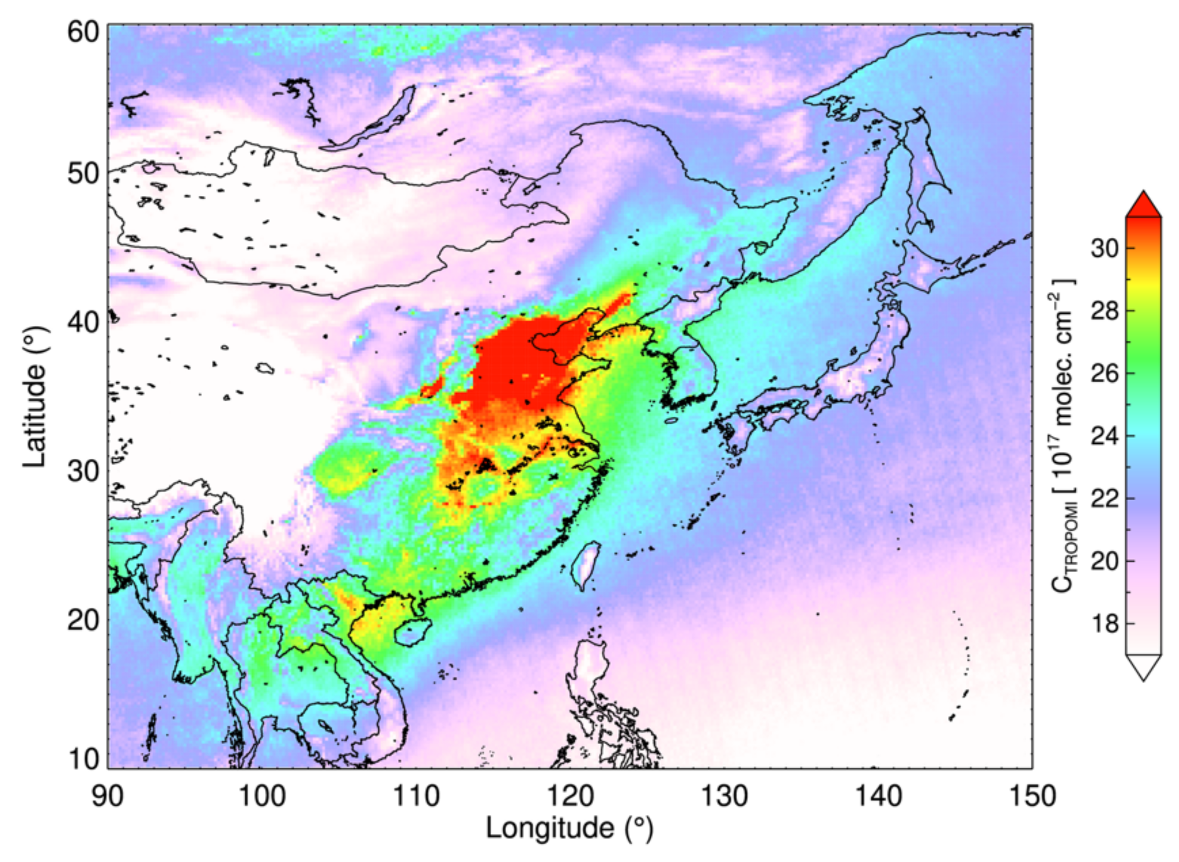
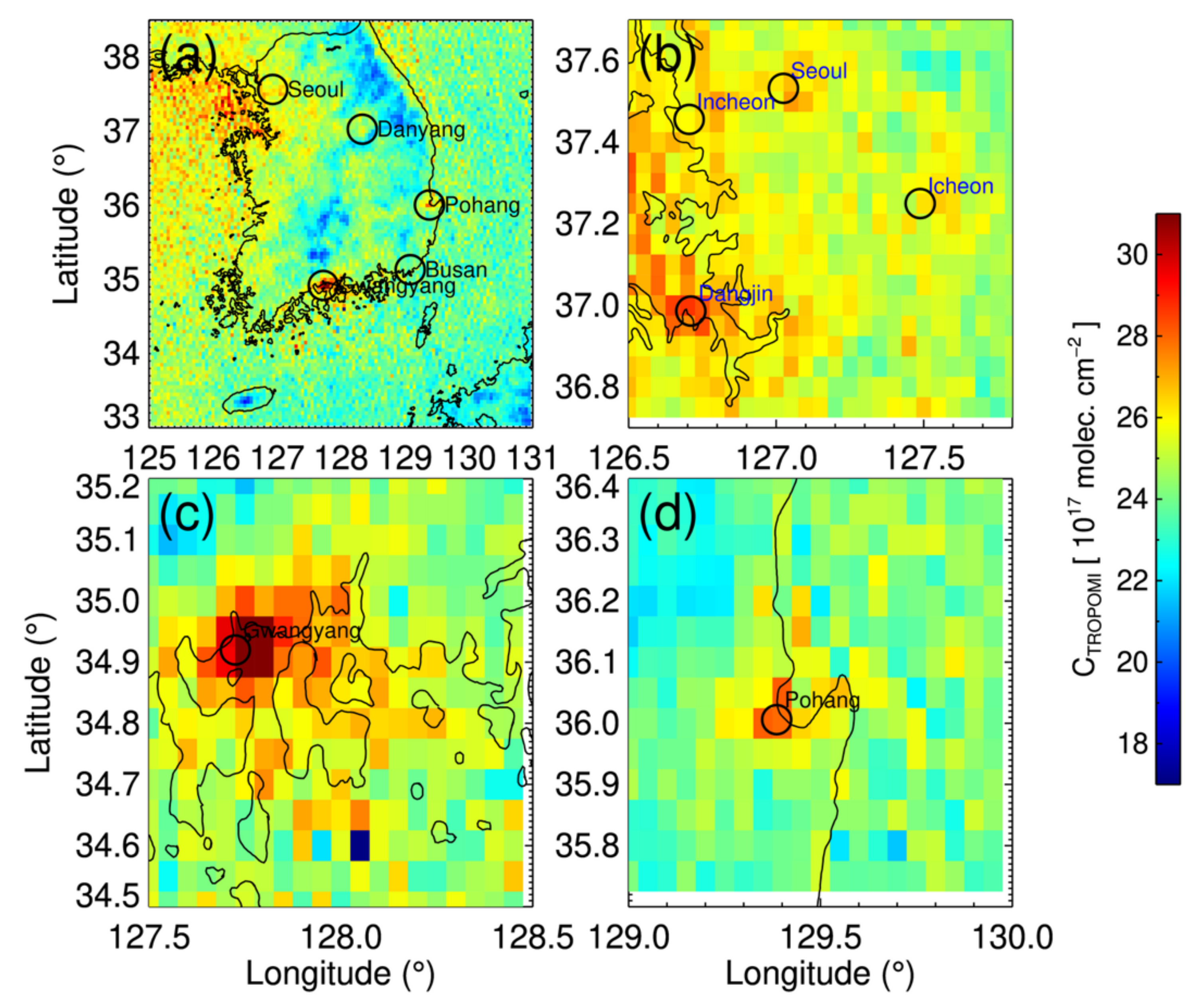
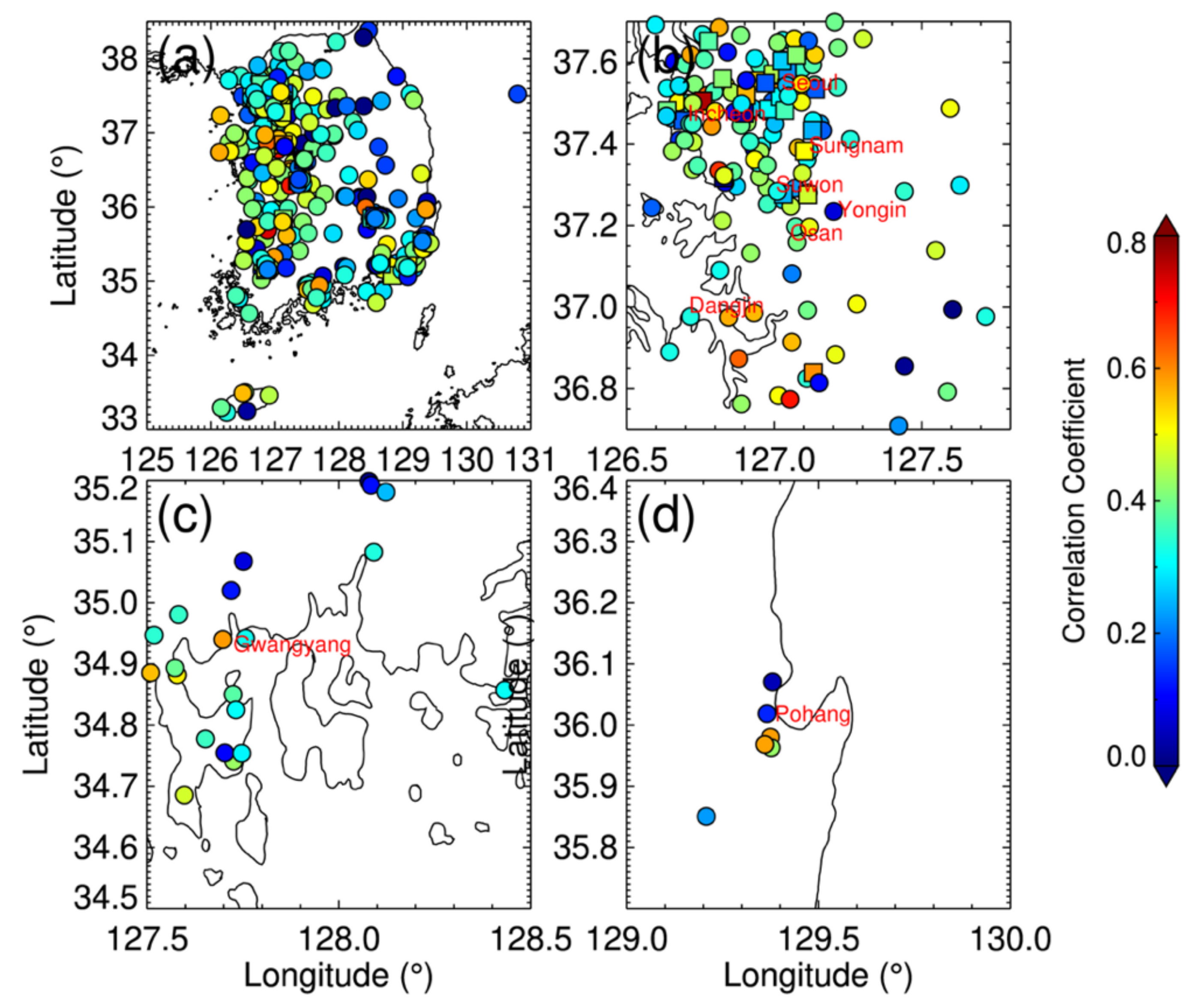
3.1. Comparison of Spatial Distributions of CO from TROPOMI and Ground Network

The mean values of CTROPOMI for 2019 over South Korea are shown in Figure 2 and were binned to a comparable resolution of the TROPOMI (0.05° × 0.05° horizontal grid). Panel (a) of Figure 2 represents South Korea, and panels (b) to (d) focus on the most significant emission areas of CO in the domain of panel (a). In general, high CTROPOMI values were observed in eastern South Korea, where the low CTROPOMI vales in Figure 2a were predominately observed over mountainous areas. Figure 2b depicts the values over the Seoul metropolitan area, where more than half of the Korean population (~26 million) is distributed. As shown in this figure, the TROPOMI clearly indicate high values of the CTROPOMI over Seoul, Incheon, and active ironworks in Dangjin. One of the largest industrial complexes in Gwangyang and the ironworks in Pohang resulted in a significant CO burden, as shown in Figure 2c,d, respectively. Large amounts of CTROPOMI over the western sea of the Korean peninsula are likely associated with trans-boundary transport from East China [30] (also see Figure 1).
The annual mean value of the CO surface mixing ratio measured by the KME network in South Korea is shown in Figure 3. The domains of the panels in Figure 3 are the same as those shown in Figure 2. As shown in this figure, the KME network was densely distributed over highly populated areas, particularly in cities situated in the Seoul metropolitan area (Figure 3b). Such strategic distribution of the ground-based network is efficient for monitoring NO2, which is predominantly emitted from transportation in South Korea [25]. However, these network spatial distributions are not optimal for monitoring CO, as this compound is predominately emitted from industrial activities. As indicated in Figure 2 and Figure 3, a vast number of stations over the Seoul metropolitan area demonstrate the spatial distribution of CTROPOMI (indicated by the comparison of Figure 2b and Figure 3b), whereas the sparse distribution of surface measurements detected limited areas of the emission sources (as shown by comparing the lower panels of Figure 2 with those of Figure 3). Satellite retrievals, such as TROPOMI, can efficiently complement such limitations of ground-based networks.
The circles and squares in Figure 2 indicate ambient and roadside monitoring stations, respectively; Jeong and Hong (2021) reported significantly higher values of NO2 from the roadside stations than the nearby ambient monitoring sites [25]. By comparing the values of the circles and squares in Figure 2b, we determined that unlike NO2, the CO mixing ratios measured at roadside stations did not show significant differences from those at ambient monitoring stations. This is likely due to the relatively longer lifetime of CO; the emitted burden of CO remains in the atmosphere for a sufficient period to be well-mixed within a boundary layer over the Seoul metropolitan areas. Therefore, CTROPOMI is likely to experience less horizontal heterogeneity within its footprint but is more closely related to boundary layer height.
Figure 4a compares the annual mean values of CTROPOMI and SKME over the KME stations. CTROPOMI values within ±0.025° from each ground station were averaged for spatial collocation. Note that the CTROPOMI and SKME are not linearly comparable due to the spatiotemporal variabilities of vertical profile. However, as a major fraction of CO supposed to be distributed within the mixing layer, we expect such comparison may provide a primitive but basic assessment of the satellite retrievals before converting the CTROPOMI to surface mixing ratio for direct comparison. The green circles and red rectangles in Figure 4a represent the ambient urban/rural monitoring stations and roadside stations, respectively. The RMSE denotes the root-mean-square error, and the MBE represents the mean bias error. For a similar comparison for NO2, the annual mean values of the TROPOMI and surface measurements show a high correlation (r = 0.84), particularly over the ambient monitoring sites (r = 0.88) [25]. However, the correlation between CTROPOMI and SKME was lower (r = 0.37), partly attributed to the lower variability of CO compared to that of NO2. As discussed, the comparison for the roadside monitoring stations did not show a notable difference from that of the ambient sites (revealed by comparing the green circles and red squares in Figure 4a). Spatiotemporally coincident samples (CTROPOMI within ±0.025° of the KME stations and SKME within ±30 min of the TROPOMI overpass time) of CTROPOMI and SKME in 2019 are compared in Figure 4b, and show a slightly lower correlation (r = 0.33) than that in panel (a).
The correlation coefficients between CTROPOMI and SKME at each KME station in 2019 are shown in Figure 5. In general, a higher correlation appeared near the emission sources of CO owing to the higher retrieval sensitivity of the TROPOMI and variability of CO. For NO2, the correlations between the TROPOMI retrievals and KME measurements over the roadside stations (squares) were significantly lower than those over the ambient stations (circles) because of their higher spatiotemporal variability near the source areas [25]. Such differences were not observed for CO, as shown in this figure, which was attributed to its relatively longer lifetime, as shown in Figure 3.
The TROPOMI retrievals utilize the profile-scaling method based on monthly averaged vertical profiles of CO from the TM5 [35,37], thus the ratio of SKME to CTROPOMI is assumed to be higher near strong emission sources: the CO mixing ratio at the surface of these areas is likely higher than that at ambient (well-mixed) stations. The ratios over the KME stations are shown in Figure 6 and were significantly high near emission sources in South Korea. The ratios along the coastal line were highly variable at each station, and could likely be attributed to complex boundary layer processes occurring over these areas (see Figure 6c,d). A similar complexity was observed for NO2 [25], which again emphasizes the importance of intensive field campaigns combined with model simulations over these areas (e.g., ozone water-land environmental transition study [46]).

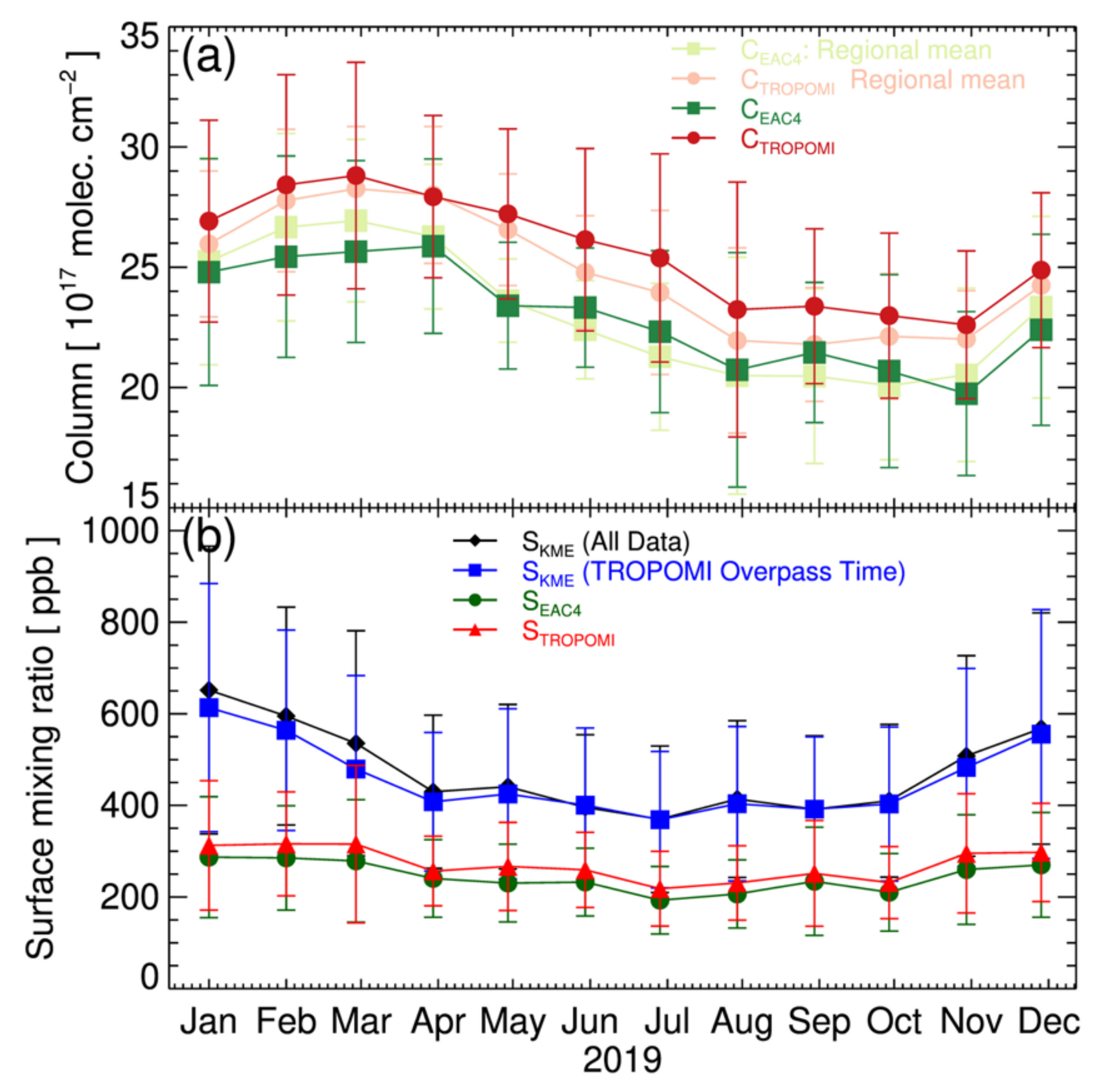
3.2. Estimation of CO Surface Mixing Ratio from TROPOMI and CAMS Reanalysis Data

To derive surface air quality from satellite data, Jeong and Hong (2021) utilized the ratio of surface mixing ratios to total column amounts from the EAC4, which are multiplied by CTROPOMI as follows [25]:
S TROPOMI = S EAC 4 C EAC 4 C TROPOMI
where STROPOMI is the estimated surface CO mixing ratio from CTROPOMI, and SEAC4 and CEAC4 are the surface mixing ratio and total column amount of CO from EAC4, respectively. As the CAMS model system (for EAC4) and TM5 (for CTROPOMI) utilizes the same chemical mechanism, which is a modified and extended version of the CB05 [47,48], we expected the biases that arose from the different averaging kernels to be minimized. Furthermore, some of the systematic biases (e.g., emission inventory) could be canceled out because the ratio of SEAC4 to CEAC4 was relatively more accurate than their absolute values.
Figure 7 shows the annual statistics of the CO vertical profiles from the EAC4 of longitudes from 125° to 131° and latitudes from 33° to 39°. The black line with circles depicts the mean values of the CO mixing ratio at each layer, the dark gray area indicates the standard deviation (±σ), and the light gray area shows the data range (minimum and maximum values) at each level. The mean values with a ±σ of SKME for entire stations are indicated by the red circle with an error bar (466 ± 218 ppb), which was significantly higher than that of the EAC4 (193 ± 95 ppb). This difference is partially attributable to the spatial coverage of the KME network; most of the ground stations are located near urban areas or large emission sources, whereas the EAC4 values in this figure were calculated from data over the entire target region of South Korea. The mean (±σ) values of CTROPOMI over this target domain and over the KME stations were 24.8 (±3.6) × 1017 molec. cm−2 and 25.3 (±4.5) × 1017 molec. cm−2, respectively. The horizontal heterogeneity of CO within a TROPOMI pixel is relatively small due to its moderate lifetime; therefore, the spatial coverage of the KME stations does not fully explain the difference between SKME and SEAC4. Turquety et al. (2008) [49] compared the Laboratoire de Météorologie Dynamique, zoom; version 4 (LMDz) and Interactive Chemistry and Aerosols; version 2 (INCA) model simulations [50,51] to the Measurement of Ozone and Water Vapor on Airbus In-Service Aircraft (MOZAIC) aircraft-based in-situ profiles [52] over Asia, and reported relatively lower biases of CO from the model in the troposphere, suggesting the underestimation of CO emissions. The uncertainties of CO emissions over South Korea in the EAC4 may have propagated errors in the CO vertical profiles, particularly near the surface, which could have affected the difference between SKME and SEAC4.
The surface mixing ratios of CO from EAC4 and derived from TROPOMI were compared with the KME measurements in Figure 8. A comparison between Figure 4 and Figure 8 reveals that the correlations of the CO surface mixing ratios between the different sources showed a higher correlation (r = 0.48–0.51) than that between SKME and CTROPOMI. Moreover, STROPOMI shows a slightly higher correlation with SKME than that between SEAC4 and SKME with a statistical significance (z-score of about 4.04). The slope of the regression line between the STROPOMI and SKME also shows slightly better consistency than that between the SEAC4 and SKME (t-value of about 6.9). Accordingly, the RMSE and MBE values between the STROPOMI and SKME were lower than those between the SEAC4 and SKME, which quantifies the benefit of using TROPOMI to derive the surface CO mixing ratio. However, such agreement between the STROPOMI and SKME was lower than that for NO2 using the identical technique over the same spatiotemporal domain [25], and the low bias of STROPOMI (MBE = −187.6 ppb) compared to SKME was still significant with respect to the average value of SKME (466 ± 218 ppb) which is discussed at following figures.
Monthly mean values of CTROPOMI (red circles) and CEAC4 (green squares) are shown in Figure 9a. The dark colors indicate the mean values over the KME stations, and the lighter colors depict those over the entire domain of South Korea (longitudes from 125° to 131° and latitudes from 33° to 39°). Over the KME stations, the mean CEAC4 values were lower than those of CTROPOMI throughout the year by approximately 10% (2.6 × 10¹⁷ molec. cm−2). This could be partly attributed to the lower spatial resolution of the EAC4 (i.e., approximately 80 km) compared to that of the TROPOMI (i.e., approximately 7 km), as the greater collocated pixels of the EAC4 for each site may contain a greater fraction of background areas around the KME stations. The average values of CEAC4 and CTROPOMI over broader and identical spatial domains experienced these sampling issues to a lesser degree, as demonstrated by the light colors in Figure 9a. The mean values of CEAC4 over the entire target domain were 7% lower than those of CTROPOMI. Regarding similar comparisons, Borsdorff et al. (2018) reported biases of approximately ±15% depending on the region (see Figure 2 of [35]), and we expected that these biases were within the uncertainty ranges of CTROPOMI and CEAC4. In addition, the monthly variations over the KME stations showed an excellent correlation (r = 0.98), as shown in Figure 9a.
As shown in Figure 7 and Figure 8, significant underestimations of SEAC4 (by approximately 46%) and STROPOMI (by approximately 40%) compared to SKME were also observed in the monthly mean values of these parameters throughout the year (Figure 9b). The black diamonds in Figure 9b depict the monthly mean values of SKME for 24-h measurements, and the blue squares indicate those for the TROPOMI overpass time. In general, the SKME values were high in winter and low in summer, despite the CTROPOMI peak observed in March (revealed by comparison of Figure 9a,b). The high CTROPOMI values in March were likely associated with active biomass burning over southeast Asia, whereas the SKME peak in January was attributed to the stable boundary layer during this period. The mean SKME values from 24-h samples and from the TROPOMI overpass time showed slight differences of approximately 6–10% in spring and winter but comparable values in summer, which was attributed to diurnal boundary layer development. Note that the NO2 from the KME at the TROPOMI overpass time was consistently lower by approximately 23% than the 24-h mean values because of a combination of its chemical processes and boundary layer development during the daytime [25]. The monthly mean SEAC4 values showed generally similar tendencies (r = 0.89), but with significantly low biases throughout the year, particularly in winter. Such relatively low biases of SEAC4 resulted in similar degrees of underestimation of STROPOMI, as presented in Figure 9b.

4. Summary and Discussions

This study aimed to assess CTROPOMI using an extensive ground-based network over South Korea to derive the surface mixing ratio of CO over the globe, key information in understanding its role in the regional air quality climate. Our analysis reveals that the CO concentration over South Korea is persistently affected by both local emissions and trans-boundary transport, emphasizing the importance of satellite-based remote sensing over the region. The TROPOMI accurately detected major sources of CO over South Korea (e.g., Seoul, Dangjin, Pohang, and Gwangyang), complementing the spatial coverage of ground-based networks. In general, the correlations between CTROPOMI and SKME (r = 0.33 for all coincident samples, r = 0.37 for annual mean values at each site) were lower than those for NO2 reported in a previous study [25], and this observation was partly attributed to the lower spatiotemporal variability. Moreover, higher correlations were observed near the emission sources. We utilized vertical profiles from EAC4 to convert the total column amounts of CO from TROPOMI to the surface mixing ratio. This converted STROPOMI was directly compared to SKME, which showed a significant underestimation of approximately 40%, with a moderate correlation of approximately 0.51. The relatively low biases of STROPOMI were more significant in winter and were associated with the underestimation of SEAC4.
Turquety et al. (2008) also reported a significant underestimation of CO (by approximately 49% below 850 hPa) from the LMDz-INCA model compared to the MOZAIC aircraft measurements over highly polluted areas in Bangkok, Thailand. They suggested that part of this underestimation could be attributed to the relatively low horizontal resolution of the model (i.e., 3.75° in longitude 2.5° in latitude) [49], which may not accurately resolve highly polluted areas. Moreover, Khan et al. (2017) also reported a significantly low bias of the MOPITT CO compared to the KME measurement in Seoul, South Korea, by approximately 35%, with a low correlation of 0.28 [53]. To the best of our knowledge, the factors affecting the low biases of the surface CO mixing ratio from satellites and models over this region remain uncertain. Intensive field campaigns combining various chemistry models of high spatial resolution (comparable to that of the TROPOMI) and in-situ profile measurements (e.g., from aircraft or unmanned aerial systems) may help to better understand these discrepancies. Moreover, multi-band retrievals of CO using both SWIR and TIR [17] may also help to detect the surface burden of CO more efficiently over a broader region. One of the important merits of this study is that this method is applicable to other regions (e.g., other Asian or developing countries, where in-situ measurements are sparse) as the EAC4 and TROPOMI provides relatively uniform quality over globe. However, comparison studies between the satellite retrievals and surface measurements are essential for broader regions to understand uncertainties in the assumed CO profiles and emissions.

Author Contributions

Conceptualization, methodology, formal analysis, investigation, resources, data curation, writing, and editing by U.J. Software, validation, resources, writing and editing, visualization, and funding acquisition by H.H. All authors have read and agreed to the published version of the manuscript.

Funding

This research was supported by the National Institute of Environmental Research (NIER) of the Ministry of Environment, Republic of Korea (grant no. NIER-2021-01-01-052).

Institutional Review Board Statement

Not applicable.

Informed Consent Statement

Not applicable.

Data Availability Statement

The TROPOMI data are available at https://scihub.copernicus.eu/ (accessed on 29 September 2019), and the EAC4 data are from https://ads.atmosphere.copernicus.eu (accessed on 29 September 2019). We obtained KME ground measurements from https://www.airkorea.or.kr (accessed on 29 September 2019).

Acknowledgments

The authors appreciate ESA and NASA for providing the TROPOMI and EAC4 data and thank the Korean Ministry of Environment for the in-situ CO data.

Conflicts of Interest

The authors declare no conflict of interest. The funder had no role in the design of the study; collection, analyses, or interpretation of data; writing of the manuscript; or in the decision to publish the results.

References

  1. Spivakovsky, C.; Logan, J.; Montzka, S.; Balkanski, Y.; Foreman-Fowler, M.; Jones, D.; Horowitz, L.; Fusco, A.; Brenninkmeijer, C.; Prather, M.; et al. Three-dimensional climatological distribution of tropospheric OH: Update and evaluation. J. Geophys. Res. Atmos. 2000, 105, 8931–8980. [Google Scholar] [CrossRef]
  2. Lelieveld, J.; Gromov, S.; Pozzer, A.; Taraborrelli, D. Global tropospheric hydroxyl distribution, budget and reactivity. Atmos. Chem. Phys. 2016, 16, 12477–12493. [Google Scholar] [CrossRef] [Green Version]
  3. Prather, M.J. Lifetimes and time scales in atmospheric chemistry. Philos. Trans. R. Soc. 2007, A365, 1705–1726. [Google Scholar] [CrossRef]
  4. Gaubert, B.; Worden, H.M.; Arellano, A.F.J.; Emmons, L.K.; Tilmes, S.; Barr’e, J.; Martinez-Alonso, S.; Vitt, F.; Anderson, J.L.; Alkemade, F.; et al. Chemical feedback from decreasing carbon monoxide emissions. Geophys. Res. Lett. 2017, 44, 9985–9995. [Google Scholar] [CrossRef] [Green Version]
  5. Myhre, G.; Shindell, D.; Bréon, F.-M.; Collins, W.; Fuglestvedt, J.; Huang, J.; Koch, D.; Lamarque, J.-F.; Lee, D.; Mendoza, B.; et al. Anthropogenic and Natural Radiative Forcing. In Contribution of Working Group I to the Fifth Assessment Report of the Intergovernmental Panel on Climate Change; Cambridge University Press: Cambridge, UK, 2014; pp. 659–740. [Google Scholar]
  6. Holloway, T.; Levy II, H.; Kasibhatla, P. Global distribution of carbon monoxide. J. Geophys. Res. 2000, 105, 12123–12147. [Google Scholar] [CrossRef]
  7. Heald, C.; Jacob, D.; Fiore, A.; Emmons, L.; Gille, J.; Deeter, M.; Warner, J.; Edwards, D.; Crawford, J.; Hamlin, A.; et al. Asian outflow and trans-Pacific transport of carbon monoxide and ozone pollution: An integrated satellite, aircraft, and model perspective. J. Geophys. Res. Atmos. 2003, 108, 4804. [Google Scholar] [CrossRef]
  8. Gloudemans, A.M.S.; Krol, M.C.; Meirink, J.F.; de Laat, A.T.J.; van der Werf, G.R.; Schrijver, G.R.; van den Broek, M.M.P.; Aben, I. Evidence for long-range transport of Carbon Monoxide in the Southern Hemisphere from SCIAMACHY observations. Geophys. Res. Lett. 2006, 33, L16807. [Google Scholar] [CrossRef] [Green Version]
  9. Hollingsworth, A.; Engelen, R.J.; Benedetti, A.; Boucher, O.; Chevallier, F.; Dethof, A.; Elbern, H.; Eskes, H.; Flemming, J. Toward a Monitoring and Forecasting System For Atmospheric Composition: The GEMS Project. Bull. Am. Meteorol. Soc. 2008, 89, 1147. [Google Scholar] [CrossRef]
  10. Reichle, H.G., Jr.; Connors, V.S. The mass of CO in the atmosphere during October 1984, April 1994, and October 1994. J. Atmos. Sci. 1999, 56, 307. [Google Scholar] [CrossRef]
  11. Deeter, M.N.; Emmons, L.K.; Francis, G.L.; Edwards, D.P.; Gille, J.C.; Warner, J.X.; Khattatov, B.; Ziskin, D.; Lamarque, J.-F.; Ho, S.-P.; et al. Operational carbon monoxide retrieval algorithm and selected results for the MOPITT instrument. J. Geophys. Res. 2003, 108, 4399. [Google Scholar] [CrossRef]
  12. McMillan, W.W.; Barnet, C.; Strow, L.; Chahine, M.T.; McCourt, M.L.; Warner, J.X.; Novelli, P.C.; Korontzi, S.; Maddy, E.S.; Datta, S. Daily global maps of carbon monoxide from NASA’s Atmospheric Infrared Sounder. Geophys. Res. Lett. 2005, 32, L11801. [Google Scholar] [CrossRef]
  13. Rinsland, C.P.; Luo, M.; Logan, J.A.; Beer, R.; Worden, H.; Kulawik, S.S.; Rider, D.; Osterman, G.; Gunson, M.; Eldering, A.; et al. Measurements of carbon monoxide distributions by the tropospheric emission spectrometer instrument onboard the Aura Spacecraft: Overview of analysis approach and examples of initial results. Geophys. Res. Lett. 2006, 33, L22806. [Google Scholar] [CrossRef] [Green Version]
  14. Turquety, S.; Hadji-Lazaro, J.; Clerbaux, C.; Hauglustaine, D.A.; Clough, S.A.; Cassé, V.; Schlüssel, P.; Mégie, G. Operational trace gas retrieval algorithm for the Infrared Atmospheric Sounding Interferometer. J. Geophys. Res. 2004, 109, D21301. [Google Scholar] [CrossRef]
  15. Deeter, M.N.; Edwards, D.P.; Gille, J.C.; Drummond, J.R. CO retrievals based on MOPITT near-infrared observations. J. Geophys. Res. 2009, 114, D04303. [Google Scholar] [CrossRef] [Green Version]
  16. Bovensmann, H.; Burrows, J.P.; Buchwitz, M.; Frerick, J.; Noël, S.; Rozanov, V. SCIAMACHY: Mission objectives and measurement modes. J. Atmos. Sci. 1999, 56, 127–150. [Google Scholar] [CrossRef] [Green Version]
  17. Worden, H.M.; Deeter, M.N.; Edwards, D.P.; Gille, J.C.; Drummond, J.R.; Nédélec, P. Observations of near-surface carbon monoxide from space using MOPITT multispectral retrievals. J. Geophys. Res. 2010, 115, D18314. [Google Scholar] [CrossRef]
  18. Veefkind, J.P.; Aben, I.; McMullan, K.; Förster, H.; de Vries, J.; Otter, G.; Claas, J.; Eskes, H.J.; de Haan, J.F.; Kleipool, Q.; et al. Tropical on the ESA Sentinel-5 Precursor: A GMES mission for global observations of the atmospheric composition for climate and air quality applications. Remote Sens. Environ. 2012, 120, 70. [Google Scholar] [CrossRef]
  19. Bernath, P.F.; McElroy, C.T.; Abrams, M.C.; Boone, C.D.; Butler, M.; Camy-Peyret, C.; Carleer, M.; Clerbaux, C.; Coheur, P.-F.; Colin, R.; et al. Atmospheric Chemistry Experiment (ACE): Mission overview. Geophys. Res. Lett. 2005, 32, L15S01. [Google Scholar] [CrossRef]
  20. Clerbaux, C.; Coheur, P.-F.; Hurtmans, D.; Barret, B.; Carleer, M.; Colin, R.; Semeniuk, K.; McConnell, J.C.; Boone, C.; Bernath, P. Carbon monoxide distribution from the ACE-FTS solar occultation measurements. Geophys. Res. Lett. 2005, 32, L16S01. [Google Scholar] [CrossRef] [Green Version]
  21. Clerbaux, C.; George, M.; Turquety, S.; Walker, K.A.; Barret, B.; Bernath, P.; Boone, C.; Borsdorff, T.; Cammas, J.P.; Catoire, V.; et al. CO measurements from the ACE-FTS satellite instrument: Data analysis and validation using ground-based, airborne and spaceborne observations. Atmos. Chem. Phys. 2008, 8, 2569–2594. [Google Scholar] [CrossRef] [Green Version]
  22. Funke, B.; López-Puertas, M.; Bermejo-Pantaleón, D.; von Clarmann, T.; Stiller, G.P.; Höpfner, M.; Grabowski, U.; Kaufmann, M. Analysis of nonlocal thermodynamic equilibrium CO 4.7 μm fundamental, isotopic, and hot band emissions measured by the Michelson Interferometer for Passive Atmospheric Sounding on Envisat. J. Geophys. Res. 2007, 112, D11305. [Google Scholar] [CrossRef]
  23. Pumphrey, H.C.; Filipiak, M.J.; Livesey, N.J.; Schwartz, M.J.; Boone, C.; Walker, K.A.; Bernath, P.; Ricaud, P.; Barret, B.; Clerbaux, C.; et al. Waters, Validation of middle-atmosphere carbon monoxide retrievals from MLS on Aura. J. Geophys. Res. 2007, 112, D24S38. [Google Scholar]
  24. Krishna, R.K.; Ghude, S.D.; Kumar, R.; Beig, G.; Kulkarni, R.; Nivdange, S.; Chate, D. Surface PM2.5: Estimate using satellite-derived aerosol optical depth over India. Aerosol Air Qual. Res. 2019, 19, 25–37. [Google Scholar] [CrossRef] [Green Version]
  25. Jeong, U.; Hong, H. Assessment of tropospheric concentrations of NO2 from the TROPOMI/Sentinel-5 Precursor for the estimation of long-term exposure to surface NO2 over South Korea. Remote Sens. 2021, 13, 1877. [Google Scholar] [CrossRef]
  26. Zhang, X.; Liu, J.; Han, H.; Zhang, Y.; Jiang, Z.; Wang, H.; Meng, L.; Li, Y.C.; Liu, Y. Satellite-observed variations and trends in carbon monoxide over Asia and their sensitivities to biomass burning. Remote Sens. 2020, 12, 830. [Google Scholar] [CrossRef] [Green Version]
  27. Buchholz, R.R.; Worden, H.M.; Park, M.; Francis, G.; Deeter, M.N.; Edwards, D.P.; Emmons, L.K.; Gaubert, B.; Gille, J.; Martínez-Alonso, S.; et al. Air Pollution Trends Measured from Terra: CO and AOD over industrial fire-prone, and background regions. Remote Sens. Environ. 2021, 256, 112275. [Google Scholar] [CrossRef]
  28. Zheng, B.; Chevallier, F.; Ciais, P.; Yin, Y.; Deeter, M.N.; Worden, H.M.; Wang, Y.; Zhang, Q.; He, K. Rapid decline in carbon monoxide emissions and export from East Asia between years 2005 and 2016. Environ. Res. Lett. 2018, 13, 44007. [Google Scholar] [CrossRef] [Green Version]
  29. Kang, H.Q.; Zhu, B.; van der A, R.J.; Zhu, C.M.; de Leeuw, G.; Hou, X.W.; Gao, J.H. Natural and anthropogenic contributions to long-term variations of SO2, NO2, CO, and AOD over East China. Atmos. Res. 2019, 215, 284–293. [Google Scholar] [CrossRef]
  30. Jeong, U.; Kim, J.; Lee, H.; Lee, Y.G. Assessing the effect of long-range pollutant transportation on air quality in Seoul using the conditional potential source contribution function method. Atmos. Environ. 2017, 150, 33–44. [Google Scholar] [CrossRef]
  31. Lalitaporn, P.; Mekaumnuaychai, T. Satellite measurements of aerosol optical depth and carbon monoxide and comparison with ground data. Environ. Monit. Assess. 2020, 192, 369. [Google Scholar] [CrossRef]
  32. Magro, C.; Nunes, L.; Gonçalves, O.C.; Neng, N.R.; Nogueira, J.M.F.; Rego, F.C.; Vieira, P. Atmospheric trends of CO and CH4 from extreme wildfires in Portugal using Sentinel-5P TROPOMI level-2 data. Fire 2021, 4, 25. [Google Scholar] [CrossRef]
  33. Van Hees, R.M.; Tol, P.J.J.; Cadot, S.; Krijger, M.; Persijn, S.T.; van Kempen, T.A.; Snel, R.; Aben, I.; Hoogeveen, R.W.M. Determination of the TROPOMI-SWIR instrument spectral response function. Atmos. Meas. Tech. 2018, 11, 3917–3933. [Google Scholar] [CrossRef] [Green Version]
  34. Landgraf, J.; aan de Brugh, J.; Scheepmaker, R.; Borsdorff, T.; Hu, H.; Houweling, S.; Butz, A.; Aben, I.; Hasekamp, O. Carbon monoxide total column retrievals from TROPOMI shortwave infrared measurements. Atmos. Meas. Tech. 2016, 9, 4955–4975. [Google Scholar] [CrossRef] [Green Version]
  35. Borsdorff, T.; de Brugh, J.A.; Hu, H.; Aben, I.; Hasekamp, O.; Landgraf, J. Measuring carbon monoxide with TROPOMI: First results and a comparison with ECMWF-IFS analysis data. Geophys. Res. Lett. 2018, 45, 2826–2832. [Google Scholar] [CrossRef]
  36. Frankenberg, C.; Platt, U.; Wagner, T. Retrieval of CO from SCIAMACHY onboard ENVISAT: Detection of strongly polluted areas and seasonal patterns in global CO abundances. Atmos. Chem. Phys. 2005, 4, 8425. [Google Scholar] [CrossRef] [Green Version]
  37. Krol, M.; Houweling, S.; Bregman, B.; van den Broek, M.; Segers, A.; van Velthoven, P.; Peters, W.; Dentener, F.; Bergamaschi, P. Two-way nested global chemistry-transport zoom model TM5: Algorithm and applications. Atmos. Chem. Phys. 2005, 5, 417–432. [Google Scholar] [CrossRef] [Green Version]
  38. Borsdorff, T.; aan de Brugh, J.; Hu, H.; Nédélec, P.; Aben, I.; Landgraf, J. Carbon monoxide column retrieval for clear-sky and cloudy atmospheres: A full-mission data set from SCIAMACHY 2.3 μm reflectance measurements. Atmos. Meas. Tech. 2017, 10, 1769–1782. [Google Scholar] [CrossRef] [Green Version]
  39. Inness, A.; Blechschmidt, A.-M.; Bouarar, I.; Chabrillat, S.; Crepulja, M.; Engelen, R.J.; Eskes, H.; Flemming, J.; Gaudel, A.; Hendrick, F.; et al. Data assimilation of satellite-retrieved ozone, carbon monoxide, and nitrogen dioxide with ECMWF’s Composition-IFS. Atmos. Chem. Phys. 2015, 15, 5275–5303. [Google Scholar] [CrossRef] [Green Version]
  40. Martínez-Alonso, S.; Deeter, M.; Worden, H.; Borsdorff, T.; Aben, I.; Commane, R.; Daube, B.; Francis, G.; George, M.; Landgraf, J.; et al. 1.5 years of TROPOMI CO measurements: Comparisons to MOPITT and Atom. Atmos. Meas. Tech. 2020, 13, 4841–4864. [Google Scholar] [CrossRef]
  41. Borsdorff, T.; aan de Brugh, J.; Schneider, A.; Lorente, A.; Birk, M.; Wagner, G.; Kivi, R.; Hase, F.; Feist, D.G.; Sussmann, R.; et al. Improving the TROPOMI CO data product: Update the spectroscopic database and destriping of single orbits. Atmos. Meas. Tech. 2019, 12, 5443–5455. [Google Scholar] [CrossRef] [Green Version]
  42. Air Korea. Available online: https://www.airkorea.or.kr (accessed on 1 January 2021).
  43. National Institute of Environmental Research (NIER). Annual Report of Air Quality in Korea; Ministry of the Environment: Sejongsi, Korea, 2019.
  44. Inness, A.; Ades, M.; Agustí-Panareda, A.; Barré, J.; Benedictow, A.; Blechschmidt, A.-M.; Dominguez, J.J.; Engelen, R.; Eskes, H.; Flemming, J.; et al. CAMS reanalysis of atmospheric composition. Atmos. Chem. Phys. 2019, 19, 3515–3556. [Google Scholar] [CrossRef] [Green Version]
  45. Deeter, M.N.; Martínez-Alonso, S.; Edwards, D.P.; Emmons, L.K.; Gille, J.C.; Worden, H.M.; Sweeney, C.; Pittman, J.V.; Daube, B.C.; Wofsy, S.C. MOPITT Version 6 product: Algorithm enhancements and validation. Atmos. Meas. Tech. 2014, 7, 3623–3632. [Google Scholar] [CrossRef] [Green Version]
  46. Sullivan, J.T.; Berkoff, T.; Gronoff, G.; Knepp, T.; Pippin, M.; Allen, D.; Twigg, L.; Swap, R.; Tzortziu, M.; Thompson, A.M.; et al. The Ozone Water–Land Environmental Transition Study: An innovative strategy for understanding chesapeake bay pollution events. Bull. Am. Meteorol. Soc. 2019, 100, 291–306. [Google Scholar] [CrossRef]
  47. CAMx. User’s Guide: Comprehensive Air-Quality Model with Extensions, Version 5.40; ENVIRON International Corporation: Novato, CA, USA, 2011; Available online: http://www.camx.com (accessed on 1 August 2021).
  48. Huijnen, V.; Williams, J.; Van Weele, M.; Van Noije, T.; Krol, M.; Dentener, F.; Segers, A.; Houweling, S.; Peters, W.; De Laat, J.; et al. The global chemistry transport model TM5: Description and evaluation of the tropospheric chemistry version 3.0. Geosci. Model. Dev. 2010, 3, 445–473. [Google Scholar] [CrossRef] [Green Version]
  49. Turquety, S.; Clerbaux, C.; Law, K.; Coheur, P.-F.; Cozic, A.; Szopa, S.; Hauglustaine, D.A.; Hadji-Lazaro, J.; Gloudemans, A.M.S.; Schrijver, H.; et al. CO emission and export from Asia: An Analysis Combining Complementary Satellite Measurements (MOPITT, SCIAMACHY, and ACE-FTS) with global modeling. Chem. Phys. 2008, 8, 5187–5204. [Google Scholar]
  50. Hauglustaine, D.A.; Hourdin, F.; Walters, S.; Jourdain, L.; Filiberti, M.-A.; Larmarque, J.-F.; Holland, E.A. Interactive chemistry in the Laboratoire de Météorologie Dynamique general circulation model: Description and background tropospheric chemistry evaluation. J. Geophys. Res. 2004, 109, D04314. [Google Scholar] [CrossRef]
  51. Folberth, G.; Hauglustaine, D.A.; Lathiére, J.; Brocheton, F. Impact of biogenic hydrocarbons on tropospheric chemistry: Results from a global chemistry-climate model. Atmos. Chem. Phys. 2006, 6, 2273–2319. [Google Scholar] [CrossRef] [Green Version]
  52. Nedelec, P.; Cammas, J.-P.; Thouret, V.; Athier, G.; Cousin, J.-M.; Legrand, C.; Abonnel, C.; Lecoeur, F.; Cayez, G.; Marizy, C. An improved infrared carbon monoxide analyzer for routine measurements aboard commercial Airbus aircraft: Technical validation and first scientific results of the MOZAIC III program. Atmos. Chem. Phys. 2003, 3, 1551–1564. [Google Scholar] [CrossRef] [Green Version]
  53. Khan, A.; Szulejko, J.E.; Bae, M.-S.; Shon, Z.H.; Sohn, J.-R.; Seo, J.W.; Jeon, E.-C.; Kim, K.-H. Long-term trend analysis of CO in the Yongsan district of Seoul, Korea, between 1987 and 2013. Atmos. Pollut. Res. 2017, 8, 988–996. [Google Scholar] [CrossRef]
Figure 1. Average CO total column amounts for 2019 from TROPOMI binned to a 0.05° × 0.05° horizontal grid over east and southeast Asia. TROPOMI CO data with quality flags ≥0.5 were used to calculate the average values.
Remotesensing 13 03987 g001
Figure 2. Average TROPOMI CO total columns for 2019 binned to a 0.05° × 0.05° horizontal grid over (a) South Korea, (b) Seoul metropolitan area, (c) Gwangyang, and (d) Pohang. TROPOMI CO data with quality flags ≥0.5 were used to calculate the average values to avoid optically thick cloud and aerosol contaminations. The black circles in panel (a) indicate major CO sources in South Korea.
Remotesensing 13 03987 g002
Figure 3. Mean values of surface CO mixing ratio from ground air-quality monitoring network of Korea Ministry of Environment in 2019. Panel (a) depicts the values over South Korea, and panels (bd) show large emission sources in domain (a). Panel (b) represents the Seoul metropolitan area, and panels (c,d) indicate industrial complexes in Gwangyang and ironworks in Pohang, respectively. The squares within these panels indicate air quality monitoring stations on the side of roads with heavy traffic and the circles represent ambient air quality monitoring sites.
Remotesensing 13 03987 g003
Figure 4. Comparison of total column CO from TROPOMI (CTROPOMI) and in-situ surface mixing ratio from KME network (SKME) over South Korea in 2019. Panel (a) compares annual mean values at each station, and panel (b) compares all collocated samples. Green circles and red rectangles in panel (a) indicate ambient and roadside monitoring stations, respectively. The RMSE stands for root-mean-squared-error, and the MBE denotes mean-bias-error.
Remotesensing 13 03987 g004
Figure 5. Correlation coefficients between CTROPOMI and SKME at the KME monitoring stations over (a) South Korea, (b) Seoul metropolitan area, (c) industrial complexes in Gwangyang, and (d) ironworks in Pohang in 2019. Circles and squares represent ambient air-quality monitoring sites and roadside air-quality monitoring stations, respectively.
Remotesensing 13 03987 g005
Figure 6. Ratio of surface mixing ratio to total column density for CO at the KME monitoring stations over (a) South Korea, (b) Seoul metropolitan area, (c) industrial complexes in Gwangyang, and (d) ironworks in Pohang in 2019. Circles and squares represent ambient air-quality monitoring sites and roadside air-quality monitoring stations, respectively.
Remotesensing 13 03987 g006
Figure 7. Statistics of CO vertical profiles from ECMWF CAMS reanalysis data (EAC4). The black line with circles indicates the mean values at each level, the dark gray area indicates ±one standard deviation, and the light gray area shows the minimum and maximum values. Profiles were sampled at longitudes from 125° to 131° and latitudes from 33° to 39° in 2019. The red circle denotes the mean CO value from all stations of the KME network for 2019, and the red line presents its ±one standard deviation.
Remotesensing 13 03987 g007
Figure 8. (a) Comparison of surface CO mixing ratios from ECMWF CAMS reanalysis data (SEAC4) and measured from KME stations (SKME) over South Korea for 2019. Panel (b) compares the ratios estimated from TROPOMI (STROPOMI) and SKME during the same period.
Remotesensing 13 03987 g008
Figure 9. (a) Monthly variations of total column CO from ECMWF CAMS reanalysis data (CEAC4; green square) and TROPOMI (CTROPOMI; red circle) in 2019. Dark colors of this panel depict their mean values over the KME stations, and light colors indicate the mean values over the entire South Korean domain (125° to 131° longitude and 33° to 39° latitude). Panel (b) presents monthly variations in the surface CO mixing ratio from the KME stations (black diamond: 24-h average, blue square: at TROPOMI overpass time, approximately 13:00 local time), EAC4 (green circle), and the TROPOMI (red triangle).
Remotesensing 13 03987 g009
Table 1. Descriptions of different parameters of CO from TROPOMI, surface measurements, and reanalysis data (EAC4).
AcronymDefinition
CTROPOMITotal vertical column density of CO from TROPOMI
CEAC4Total vertical column density of CO from EAC4
SKMESurface mixing ratio of CO from ground network of Korea Ministry of Environment
STROPOMISurface mixing ratio of CO converted from CTROPOMI
SEAC4Surface mixing ratio of CO from EAC4
Publisher’s Note: MDPI stays neutral with regard to jurisdictional claims in published maps and institutional affiliations.

