Article

Feasibility of the Spatiotemporal Fusion Model in Monitoring Ebinur Lake’s Suspended Particulate Matter under the Missing-Data Scenario

1
Key Laboratory of Oasis Ecology, Xinjiang University, Urumqi 830046, China
2
Xinjiang Institute of Technology, Aksu 843000, China
3
Key Laboratory of Wisdom City and Environment Modeling of Higher Education Institute, College of Resources and Environmental Science, Xinjiang University, Urumqi 830046, China
4
Engineering Research Center of Central Asia Geoinformation Development and Utilization, National Administration of Surveying, Mapping and Geoinformation, Urumqi 830002, China
5
Department of Social Sciences, Education University of Hong Kong, Lo Ping Road, Tai Po, Hong Kong 999077, China
6
GeoInformatic Unit, Geography Section, School of Humanities, Universiti Sains Malaysia, USM, Penang 11800, Malaysia
*
Author to whom correspondence should be addressed.
Contributed equally to this work.
Remote Sens. 2021, 13(19), 3952; https://doi.org/10.3390/rs13193952
Submission received: 8 September 2021 / Revised: 27 September 2021 / Accepted: 29 September 2021 / Published: 2 October 2021

Abstract

:
High-frequency monitoring of suspended particulate matter (SPM) concentration can improve water resource management. Missing high-resolution satellite images could hamper remote-sensing SPM monitoring. This study resolved the problem by applying spatiotemporal fusion technology to obtain high spatial resolution and dense time-series data to fill image-data gaps. Three data sources (MODIS, Landsat 8, and Sentinel 2) and two spatiotemporal fusion methods (the enhanced spatial and temporal adaptive reflectance fusion model (ESTARFM) and the flexible spatiotemporal data fusion (FSDAF)) were used to reconstruct missing satellite images. We compared their fusion accuracy and verified the consistency of fusion images between data sources. For the fusion images, we used random forest (RF) and XGBoost as inversion methods and set “fusion first” and “inversion first” strategies to test the method’s feasibility in Ebinur Lake, Xinjiang, arid northwestern China. Our results showed that (1) the blue, green, red, and NIR bands of ESTARFM fusion image were better than FSDAF, with a good consistency (R2 ≥ 0.54) between the fused Landsat 8, Sentinel 2 images, and their original images; (2) the original image and fusion image offered RF inversion effect better than XGBoost. The inversion accuracy based on Landsat 8 and Sentinel 2 were R2 0.67 and 0.73, respectively. The correlation of SPM distribution maps of the two data sources attained a good consistency of R2 0.51; (3) in retrieving SPM from fused images, the “fusion first” strategy had better accuracy. The optimal combination was ESTARFM (Landsat 8)_RF and ESTARFM (Sentinel 2)_RF, consistent with original SPM maps (R2 = 0.38, 0.41, respectively). Overall, the spatiotemporal fusion model provided effective SPM monitoring under the image-absence scenario, with good consistency in the inversion of SPM. The findings provided the research basis for long-term and high-frequency remote-sensing SPM monitoring and high-precision smart water resource management.

Graphical Abstract

1. Introduction

Water is very important in ensuring the sustainable development of human society [1]. However, human activities and climate change have threatened the global water quality [2]. Research on the continuous monitoring of water quality has attracted considerable attention [3,4]. Suspended particulate matter (SPM) is one of the important attributes to determine water clarity by controlling light penetration through the water column [5]. It plays an important role in regulating water productivity and aquatic ecosystem functions [6]. In addition, SPM serves as a key carrier of carbon, oxygen, nutrients, and heavy metals [7,8], and the main raw material to continuously change the in situ environment and exert pressure on the ecosystem [9,10]. Therefore, the dynamic monitoring of SPM constitutes a critical domain of the intelligent management package for water resources [11].
Conventionally, SPM has been surveyed in situ [12,13]. However, manual or automatic sampling in a field-monitoring network of point measurements is costly, laborious, and time consuming. Moreover, the traditional sampling scheme cannot yield sufficient and reliable data to analyze dynamic water-quality parameters such as SPM, with a wide range of spatiotemporal variabilities [14]. Remote sensing offers an alternative that can capture sequential data, which have been rigorously pre-processed. It has the advantages of a wide temporal range of monitoring, making it possible to analyze the spatial and temporal variabilities of SPM concentrations in the surface layer of water bodies [15,16]. Many studies have applied optical remote sensing to estimate various water quality parameters such as SPM, turbidity, total nitrogen/total phosphorus ratio (TN/TP) [17,18,19,20]. However, only a few studies have explored the applicability of the spatiotemporal fusion algorithm in high-frequency SPM monitoring [21]. As a result, the retrieval of SPM concentration data using the spatiotemporal fusion of multi-source remote-sensing data is extremely rare [22].
The recent rapid development of remote-sensing technology has played an increasingly important role in environmental–ecological studies concerning dynamic ecosystem changes [23,24]. Due to the limitations of the technology, most sensors of orbit satellites often cannot acquire a sufficient number of high spatiotemporal resolution images in a given period [25]. This data inadequacy has notably restricted the application of remote-sensing data in various fields. To resolve such problems, spatiotemporal fusion technology can effectively obtain high spatial resolution and continuous time-series data [26]. In addition to the fusion technology, scholars also intended to improve the spatiotemporal resolution of remote-sensing images in other perspectives such as improving the quality of the images [27,28], integrating multi-source satellites data [22], and developing CubeSat constellations [29]. The improvement of remote-sensing image quality can only play a role when the original image quality is poor. Therefore, the improvement of spatiotemporal resolution by this method is limited. The multi-source data integration method is limited from different sensor parameters; thus, the spatiotemporal resolution improvement solely depends on the characteristics of the combined sensors. Although CubeSat constellations fill the gap of the high spatiotemporal resolution, its global land surface imaging coverage capability was only available recently, including about 130 orbiting satellites [30]. In fact, it cannot obtain long historical time series images [31]. Therefore, spatiotemporal fusion technology can improve and fill the gap of long-time historical images [32].
Based on the principles of data fusion, Guo et al. [24] divided the spatiotemporal fusion models into five categories: learning-based, weight-function-based, Bayesian-based, hybrid, and unmixing-based methods. Their working principles can be found in the literature [33]. Although many spatiotemporal fusion models have been established to improve the spatiotemporal resolution of remote-sensing images, they differ notably in the data source, calculation efficiency, prediction accuracy, and data input requirement [34]; hence, it is difficult to determine their relative advantages. It is necessary to evaluate model applicability to specific study areas and data sources. Here, we chose ESTARFM and FSDAF methods to reconstruct missing images. ESTARFM is an enhancement model based on STARFM, which fully considers the spatial heterogeneity of pixels for obtaining better fusion results [35]. Meanwhile, FSDAF can obtain robust fusion results by combining un-mixing, spatial interpolation, and similar neighboring pixel smoothing techniques [36]. Therefore, taking MODIS, Landsat 8, and Sentinel 2 as data sources, this study explored the spatiotemporal fusion effect and consistency of the ESTARFM and FSDAF models and then analyzed the feasibility of retrieving SPM under the missing-image scenario.
The establishment of the inversion model is the key process to realize SPM monitoring in waters. At present, remote-sensing SPM inversion models can be summarized into three types: empirical method, analytical method, and semi-empirical/semi-analytical method [37]. The empirical method obtains the water quality information by establishing the statistical relationship between the measured and remote-sensing data. Due to the lack of a physical basis, this method’s inversion accuracy and universality are judged to be unsatisfactory [38,39]. The analytical method uses the bio-optical and radiative transfer models to simulate the light transmission process in the atmosphere and water body and then establishes the relationship between water quality parameters and the water-leaving reflectance spectrum [40,41]. This method has a high inversion accuracy and generality in theory, but its observation equipment is complex and expensive, thus limiting its practical application [42]. The semi-empirical/semi-analytical method combines the known spectral characteristics of water quality parameters with a statistical model. It selects the best band or band combination as the independent variable to estimate the water quality parameters [43,44]. This method only needs a small amount of spectral and measured data to establish the model. RF and XGBoost are classic representatives of semi-empirical models with robust performance in various fields of application research [45,46,47]. Therefore, RF and XGBoost were selected to monitor SPM in this study. It is worth noting that this study uses the fused image as the data source to monitor the SPM concentration in Ebinur Lake, and similar studies were rarely reported.
Our study area was Ebinur Lake, which is the largest saltwater lake in Xinjiang. It is located in arid northwestern China, with important urban agglomeration on the northern slope of the Tianshan Mountain [48]. In recent decades, global climate change and the intensification of regional anthropogenic activities have profoundly changed the structure, path, and driving forces of watershed environmental evolution [49]. Due to frequent wind impacts, shallow water, and high salinity, the water body would often remain in a state of high turbidity accompanied by fast changes in the lake area. Frequent lake area changes would retain the salt in the dried-up lake basin and quickly form salinized soil. There is a positive correlation between the dry bottom area of the Ebinur Lake and the total dust days in the watershed [50,51]. Salt dust has seriously affected the ecological environment and human activities in the region’s urban agglomerations with extended influence to the whole of northern China [52]. Therefore, it is necessary to carry out high-frequency remote-sensing monitoring of SPM in Ebinur Lake to provide a theoretical basis to improve water quality management and salt dust control.
Based on the spatiotemporal fusion model, this study aimed to explore the feasibility of monitoring SPM in Ebinur Lake under the missing-image situation using two retrieval strategies (“fusion first” and “inversion first”). We explored four research questions: (1) For the shallow saltwater Ebinur Lake in arid northwestern China, what is the fusion accuracy of ESTARFM and FSDAF? (2) What is the consistency of the fused images between MODIS-Landsat 8 (ML8) and MODIS-Sentinel 2 (MS2)? (3) What is the accuracy of Landsat 8 and Sentinel 2 data in monitoring SPM in Ebinur Lake? (4) With gaps in satellite images, which strategy is more suitable for the effective monitoring of SPM in Ebinur Lake? Are they consistent with the SPM images retrieved from the original Landsat 8 and Sentinel 2 images?

2. Study Area and Methods

2.1. Study Area

Ebinur Lake is located in northwest Xinjiang in arid northwestern China (Figure 1). The site has few water quality monitoring stations and poor data continuity, leading to data scarcity [53]. Mountains surround it to the west, south, and north. Only the Bortala and Jing rivers currently feed into it, and a large area of agricultural land spreads in the southwest. The average lake depth is merely 1.4–1.6 m, with a water density of about 1.079 g/cm3, pH 8.49, and mineralization 112.4 g/L. The high salt content of the Ebinur lake water does not permit vegetation growth in the water area, leading to a very low chlorophyll content (when the volume of experimental water is 100 mL, its content is lower than the detection limit of 0.04 mg/L (HJ 897-2017)). The lake area fluctuates greatly between the wet and dry seasons, and the turbidity stays at a high level (the average SPM concentration in 28 days is 874.88 mg/L), with traits of a typical shallow saltwater lake in Central Asia. The Ebinur Lake region has low rainfall and strong evapotranspiration. The northwestern part of the lake basin is the well-known strong wind area “Alashankou” in China, with about 164 windy days (greater than 17.0 m/s) in a year [54,55,56]. The wind disturbs the sediments at the lake’s bottom, bringing the sediments to the exposed lake basin with the waves [54]. This is one of the important sources of salt dust. The frequent salt-dust weather has negatively impacted local power supply and distribution facilities and crop growth [57,58]. Previous research experience has shown that Ebinur Lake is often in a state of strong dynamic change [54]. Therefore, the high-frequency monitoring of its SPM is very necessary.

2.2. Data Source and Pre-Processing

Five fixed points were set up in Ebinur Lake to monitor variations of SPM concentration (Figure 1c). The in situ data were collected in May, June, September, and October from 2011 to 2020, with a total of 102 samples. May and September were monitored every year. The sampling adhered to the Technical Specifications Requirements for Monitoring of Surface Water and Waste Water (HJ/T 91-2002). The SPM concentration was obtained by the gravimetric method (GB 11901-89). After screening, 35 remote-sensing images were used, including Landsat 7, Landsat 8, MODIS, and Sentinel 2. The absolute time differences between the sampling dates and the satellite images were within five days, with 77.14% within two days (Figure 2). In remote-sensing applications, this time difference is acceptable [59,60,61]. MODIS data (MOD09GA: reflectance production data with a spatial resolution of 500 m) were downloaded from https://ladsweb.modaps.eosdis.nasa.gov/ (accessed on 2 July 2021), while Sentinel 2 and Landsat data were acquired from the US Geological Survey website at http://lglovis.usgs.goc/ (accessed on 2 July 2021).
According to the principle that the field sampling time should be synchronous with the transit time of satellites, 11 Landsat images (4 Landsat 7 and 7 Landsat 8), 8 Sentinel 2 images, and 18 MODIS images were selected. The corresponding number of sampling points for Landsat, Sentinel 2, and MODIS were 49, 42, and 37, respectively. For the Fast Line-of-sight Atmospheric Analysis of Spectral Hypercubes (FLAASH), the atmospheric correction module in ENVI (Version 5.3, ITT Visual Information Solutions, Boulder, CO, USA) was used for radiometric calibration and atmospheric correction of the Landsat series images. SNAP (http://step.esa.int (accessed on 12 July 2020)) was used for atmospheric correction of Sentinel 2. On the other hand, MRT (https://lpdaac.usgs.gov/ (accessed on 10 June 2021)) was used to reproject MODIS data to the UTM-WGS84 geographic coordinate system. Both Sentinel 2 and MODIS data were resampled to 30 m and accurately geo-referenced with Landsat 8. Finally, the normalized difference water index (NDWI) was used to mask the water body to obtain the reflectivity image of Ebinur Lake.

2.3. Sensitive Band Selection

In previous studies, whether adopting a single band or band combination, the bands related to the retrieval of SPM in water bodies were mainly blue, green, red, and NIR [21,38]. In this study, the coordinates of the sampled points were spatialized and overlaid with Landsat 7/8, MODIS, and Sentinel-2 images. ArcGIS 10.3 was used to extract the reflectance values of the sampling points on each band of the three sets of satellite data. Then, Pearson correlation analysis was performed between reflectivity and SPM concentration in each band by SPSS 20 (IBM Corporation, Chicago, USA). Finally, the band sensitive to SPM was selected according to the significance level. After analysis, the blue, green, red, and NIR were selected as the sensitive bands for SPM inversion in this study (Figure 3).

2.4. Spatiotemporal Fusion Model

One of the necessary conditions for the spatiotemporal fusion of images is the existence of overlapping areas in the wavelength bands of satellite data. The central wavelength of a band of one sensor should lie within a certain wavelength range of another sensor [34]. Figure 4 shows the band correspondence of the data sources used in this study. This theoretical basis for spatiotemporal fusion was satisfied with a large overlap between all four data source bands.
This paper investigated the feasibility of applying spatiotemporal fusion models to lake SPM monitoring beset by image-data gaps. Two inversion strategies for SPM were set to tackle the problem—namely, “fusion first” and “inversion first”. The “fusion first” strategy enlisted the spatiotemporal fusion model to obtain the substitution remote-sensing image at an unknown time. It then used the image to invert the SPM at that time. The “inversion first” strategy employed the remote-sensing image at a given time to retrieve the SPM at that time. A spatiotemporal fusion model fused the SPM maps at a known time to obtain the SPM at an unknown time. The spatiotemporal fusion models used in this paper were ESTARFM and FSDAF. The ESTARFM fusion method [35,62] was developed based on the basic framework of STARFM. It uses the known fine and coarse images at two times (T′, TN) as the data source to calculate the weight and conversion coefficient of similar pixels. Finally, it uses the coarse image at the predicted time (T) as the input to calculate the fine image at T time. The final prediction of ESTARFM is shown in Formula (1).
L b ( x w / 2 , y w / 2 , T ) = L b ( x w / 2 , y w / 2 , T ) + i = 1 n W i × v i × ( M b ( x i , y i , T ) M b ( x i , y i , T ) )
where Lb and Mb represent the reflectance of fine and coarse images in band b, w′ represents the moving window size, (xw′/2, yw′/2) represents the position of the analog pixel, Wi is the weight of the ith pixel similar to the predicted pixel, vi is the conversion coefficient between predicted pixel and its similar pixels, n represents the number of pixels similar to the predicted pixels, and (xi, yi) is the position of the ith pixel similar to the predicted pixel.
The FSDAF fusion method [36] takes the fine and coarse image pairs at a known time as the data source to calculate the residual, weight function, etc. Finally, the fine image at the predicted time is obtained by taking the coarse image at the predicted time as the input. The final prediction of FSDAF is shown in Formula (2).
F 2 ( x , y ) = F 1 ( x , y ) + i = 1 n s w i ( Δ F t p ( x i , y i ) + n × R ( x i , y i ) × w h ( x i , y i ) )
where ns is the number of similar pixels in the moving window, and w i is the weight of the ith similar pixel. Δ F t stands for a temporal change of a fine pixel, n stands for the number of fine pixels inside a coarse pixel, R(xi, yi) stands for the residual in the coarse pixel at location (xi, yi), and w h is a weighted function.
In this study, the operation of the spatiotemporal fusion model was realized by IDL language. The original Landsat 8 and Sentinel 2 images on 29 August 2017 were used to test the accuracy of the spatiotemporal fusion model. The data source dates of the two spatiotemporal fusion models are listed in Table 1.

2.5. Inversion Model for SPM

SPM is one of the most important water parameters, which profoundly affects the habitat quality of water bodies [20]. Extensive research has been accomplished to bring fruitful results [20,38,63]. To obtain the SPM concentration in Ebinur Lake efficiently, two algorithms (bagging and boosting) were adopted in this study to implement the inversion successfully. We chose two representative models: random forest (RF) and XGBoost; their theoretical basis is explained in Liaw and Wiener [64] and Lu et al. [65]. Random forest (RF) is an ensemble learning algorithm introduced by Breiman [66] to improve the traditional decision tree method. RF is a bagging algorithm [67] for classification or regression problems [68]. The main calculation process includes (1) random selection of samples via bootstrap; (2) random selection of features; (3) constructing decision tree; (4) prediction (voting or average). XGBoost is a boosting algorithm [69], originally introduced by Chen and Guestrin [70]. XGBoost is better than gradient boosting decision tree (GBDT) because it avoids overfitting by integrating regularization terms in the modeling process. XGBoost can perform three gradient enhancements, e.g., regularization, random, and gradient. Therefore, it can significantly improve the effect of classification or regression problems [71]. The inversion was conducted based on a single sensitive band to explore the potential of spatiotemporal fused images and two inversion models in monitoring SPM.

2.6. Performance Evaluation
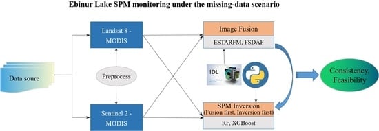
To quantify the differences between the spatiotemporal fused and the real images, we used Python 3.0 to calculate the following evaluation indexes for accuracy evaluation. The coefficient of determination (R2), the normalized root mean square error (NRMSE), the peak signal-to-noise ratio (PSNR), and the structural similarity index (SSIM) served as the evaluation indexes of image quality. Assuming that the real image I pixel ranks are m × n, the spatiotemporal fused image is F, I(i,j) is the real image pixel value, and F(i,j) is the spatiotemporal fused image pixel value. The R2 was used to evaluate the consistency of pixel values between spatiotemporal fused and real images. The calculation process is
R 2 = i = 1 m j = 1 n I ( i , j ) I ¯ F ( i , j ) F ¯ i = 1 m j = 1 n I ( i , j ) I ¯ 2 i = 1 m j = 1 n F ( i , j ) F ¯ 2 2
The NRMSE is the RMSE value normalized to lie between (0,1) to evaluate the accuracy of different spatiotemporal fusion methods. The calculation process of RMSE is
R M S E = i = 1 m j = 1 n ( I ( i , j ) F ( i , j ) ) 2 m n
The PSNR evaluated the amount of information in the fused image [72]. It has a general benchmark of 30 dB, below which the image degradation is more pronounced. PSNR is often defined by the mean square error (MSE). Assuming two m × n monochrome images I and F, their MSE can be defined by Equation (5), and the corresponding PSNR is defined by Equation (6), where MAX(i,j) represents the maximum pixel value of the image.
M S E = 1 m n i = 0 m 1 j = 0 n 1 [ I ( i , j ) F ( i , j ) ] 2
P S N R = 10 log 10 M A X ( i , j ) 2 M S E
The structural similarity (SSIM) is also an indicator of image quality to assess the degree of structural similarity between fused and real images [73]. The value range is (0,1), and a large value indicates smaller image distortion. The implementation process is
S S I M = ( 2 u I u F + C 1 ) ( 2 σ I F + C 2 ) ( u I 2 + u F 2 + C 1 ) ( σ I 2 + σ F 2 + C 2 ) )
where u I and u F represent the mean value of the original image and the fused image, respectively; σ I and σ F represent their standard deviation; σ I F represents the covariance between the two images. C1 and C2 are two constants close to 0 to make the results stable. An SSIM value closer to 1 means that the two images have a similar structure.
To evaluate the performance of the SPM inversion model, we employed the Python statistical function library scipy.stats to conduct statistical analysis. Four indicators, coefficient of determination (R2), root mean square error (RMSE), mean absolute error (MAE), and residual prediction deviation (RPD), were enlisted to evaluate the accuracy and stability of the model [38]. R2 and RMSE are calculated by Equations (3) and (4), and MAE and RPD by Equations (8) and (9) as follows:
M A E = 1 n i = 1 n y i y i
R P D = S D R M S E
where yi represents the observation value, yi′ is the mean value, SD is the standard deviation of the validation sample, and RMSE is the root mean square error. RPD > 2 mg/L indicates that the model has an excellent predictive ability. In the range 1.4–2 mg/L, the model can offer rough quantitative predictions. RPD < 1.4 mg/L means that the model is not predictive.

2.7. Workflow

Based on satellite (MODIS, Landsat 8, and Sentinel 2) and in situ data (SPM), this study used spatiotemporal fusion models ESTARFM and FSDAF to obtain Landsat 8 and Sentinel 2 fusion images and analyzed their consistency. The RF and XGBoost inversion models were used to complete the mapping of SPM distribution in Ebinur Lake. The feasibility of spatiotemporal fusion models for monitoring lake SPM was then explored. The rather complex steps in the workflow of this study are depicted in Figure 5.

3. Results

3.1. Performance of the Ebinur Lake SPM Inversion Models

In this paper, the Python scikit-image algorithm was used to call the RF and XGBoost packages to implement the inversion of SPM. The training and validation sets were divided by a 7:3 ratio, and the optimal inversion model was obtained after training. The specific parameters of the optimal model and the evaluation index of the verification set are shown in Table 2. Other parameters of the model adopted the default values of RF and XGBoost packages. The validation set accuracy of both the RF and XGBoost suspension inversion models could meet the prescribed requirements (R2 ≥ 0.78), and the model stability was rated as high (RPD ≥ 2.13).

3.2. Performance Evaluation of the Two Sensors and Two Spatiotemporal Fusion Approaches

Two spatiotemporal fusion models, ESTARFM and FSDAF, were used to conduct spatiotemporal fusion studies on ML8 and MS2, respectively. We used NDWI and visual interpretation to obtain the vector boundary of Ebinur Lake. In ArcGIS 10.3 (ESRI Corporation, Redlands, USA), the model builder was used to construct the clipping model, and then the images with the same number of pixels were obtained according to the water vector boundary. Figure 6 shows the true color display (red, green, blue) of the original images and the fused images of Ebinur Lake.
Figure 6 shows that the two spatiotemporal fusion models can predict the target date image well, but the ESTARFM model performed better from a visual perspective. To quantify the quality and spectral information retention of the fused images produced by the two spatiotemporal fusion models, we generated the correlation maps between the bands of the fused image and the corresponding bands of the original image. At the same time, R2, NRMSE, PSNR, and SSIM of the fused images and the original images were calculated to quantitatively evaluate the fusion effect, as shown in Figure 7 and Figure 8.
Figure 7 shows the fusions of ML8 and MS2 of four different bands with the ESTARFM and FSDAF models. The best fusion was achieved in the red band and the worst in the NIR band. All coefficients of determination (R2) values were above 0.66, except for the NIR band fused by the ML8-based FSDAF model. Furthermore, Figure 7 shows that the values of R2 for each band of the MS2-based spatiotemporal fused images were greater than the ML8-based ones. In addition, the results also indicate that the ESTARFM model performed better than the FSDAF model in the image fusion over Ebinur Lake, which is consistent with the visualization analysis.
In addition to reflecting the spatiotemporal fusion accuracy, Table 3 raises deep reflections on three problems: (1) Which satellite data source has more advantages when spatiotemporal fusion is carried out? (2) Which spatiotemporal fusion model is better in producing the Ebinur lake water fusion images? (3) What is the fusion accuracy of each band? On the first question, most of the evaluation metrics show that MS2 are better than ML8 corresponded to four bands, where the MS2-based fused images had higher R2, PSNR, SSIM values, and smaller NRMSE values. Therefore, MS2 should be prioritized in the image fusion of Ebinur Lake. For the second question, the R2, PSNR, SSIM, and NRMSE values were better in the ESTARFM model, compared with the FSDAF model, showing that the ESTARFM method was more suitable for image fusion of the Ebinur Lake area. For the third question, the best fusion performance of ML8 and MS2 was in the green and red bands. This result is explained by the R2, NRMSE, and SSIM in the green and red bands, which were better than those in other bands.

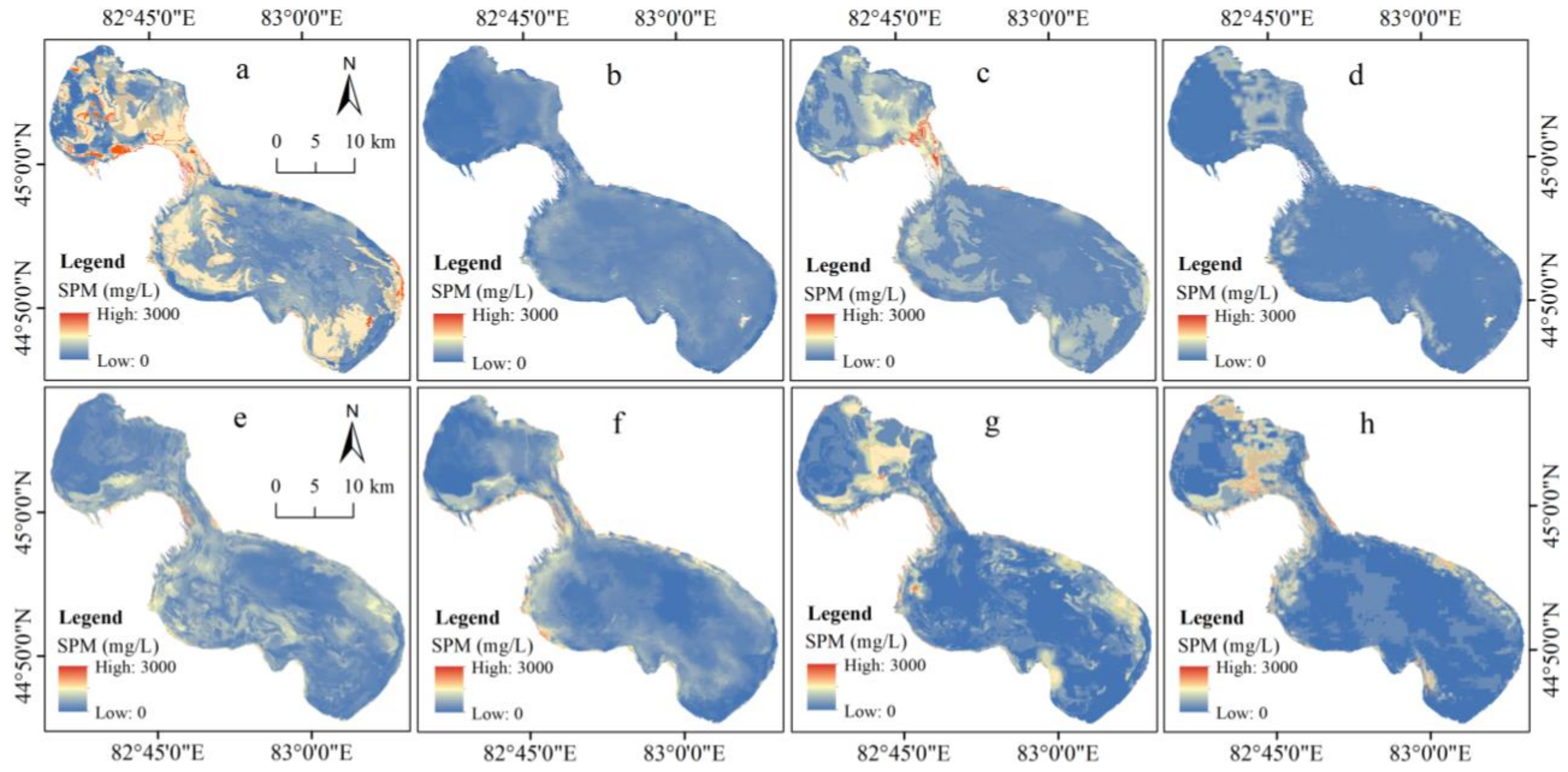
3.3. Consistency Evaluation of Spatiotemporal Fusion Images

To evaluate the consistency of fusion images based on Landsat 8 and Sentinel 2, the R2, NRMSE, PSNR, and SSIM of two original images—ESTARFM fusion images and FSDAF fusion images—in each band were compared. The correlation scatter plots of each band are shown in Figure 8, and the relative trend of the four indicators is shown in Figure 9.
Figure 8 shows that the R2 ≥ 0.82 of the original images of Landsat 8 and Sentinel 2 were high in each band, indicating that the original images of the two data sources had high consistency. The R2 for both ESTARFM- and FSDAF-fused images of ML8 and MS2 were greater than 0.54 in all bands, and the fusion accuracy was higher using ESTARFM than FSDAF. Other indicators for evaluating the consistency of Landsat 8 with Sentinel 2 and their fused images are given in Figure 9. The highest consistency was based on the original images, the second-highest on the ESTARFM-fused image, and the worst on the FSDAF-fused image. In summary, the ESTARFM- and FSDAF-based spatiotemporal fusion models fused well in the Ebinur Lake area, with strong consistency between Landsat 8, Sentinel 2, and their fused images across the bands.

3.4. Retrieval Effect of SPM from the Original Image

In this paper, two inversion algorithms (RF and XGBoost) were used to implement the 29 August 2017 Ebinur Lake SPM inversion, and then their inversion accuracy was evaluated. The retrieval results of SPM from Landsat 8 and Sentinel 2 images are shown in Figure 10, and their accuracy evaluation is shown in Figure 11 and Table 4.
Figure 11 indicates that higher SPM concentrations in Ebinur Lake on 29 August 2017 were in shallow shoreline waters, and the lower values were roughly distributed in the central portion of the lake. Using the RF algorithm for inversion, the distribution of SPM inversions based on Landsat 8 and Sentinel 2 was generally consistent. Using XGBoost highlighted a clear difference between them.
Figure 11 shows that the RF algorithm was significantly better than XGBoost for the SPM inversion, with a high correlation (R ≥ 0.83). Table 4 indicates that the accuracy of the RF-based SPM inversion at R2 ≥ 0.68 was significantly higher than the XGBoost-based inversion at R2 ≤ 0.24. The accuracy of the SPM inversion based on Sentinel 2 was slightly higher than Landsat 8 using the RF algorithm, consistent with the R2 scatter-plot results. Thus, the RF algorithms for Landsat 8 and Sentinel 2 could effectively monitor SPM in Ebinur Lake.

3.5. Consistency Evaluation of SPM Retrieval from Original Images

Due to the low accuracy of the XGBoost-based inversion, this study only used the RF algorithm as the inversion method to investigate the consistency of the SPM inversion concentration based on Landsat 8 and Sentinel 2. Using the Create Random Points tool of ArcGIS 10.3 (ESRI Corporation, Redlands, CA, USA), 1000 random points were selected on the RF-based SPM inversion maps of Landsat 8 and Sentinel 2 according to the principle of minimum allowable distance (30 m). Their SPM concentration was then extracted to explore their consistency in spatial distribution. The correlation (R) between the two was 0.71 with p < 0.01 (Figure 12). Additional indicators evaluating the accuracy of the SPM inversion for both data sources were obtained by calling the Python scikit-image algorithm. The consistency results were good for both inversion maps (Table 5).

3.6. SPM Inversion of the Fused Images

To explore the feasibility of SPM inversion in water bodies under the missing-image condition, two strategies (“fusion first” and “inversion first”) were used to monitor SPM in Ebinur Lake. To facilitate cross-validation, the SPM monitoring date was set to 29 August 2017. The inversion maps are shown in Figure 13 and Figure 14.
Comparing Figure 10 and Figure 13, the SPM distribution maps obtained based on ESTARFM (Landsat 8/Sentinel 2)-RF were more similar to the original image SPM inversion maps from the visual viewpoint. The performance of the other three inversion maps was difficult to distinguish. Comparing Figure 10 and Figure 14, it was difficult to distinguish qualitatively the advantages and disadvantages of the four SPM distributions maps.
To quantitatively evaluate the effectiveness of the two strategies for SPM inversion at missing-image times, the Python scikit-image algorithm was called to evaluate their inversion accuracy. The evaluation indicators for the optimal combination are shown in Table 6. The meaning of ESTARFM (Sentinel 2)_RF in Table 6 is as follows: firstly, MODIS and Sentinel 2 were fused by ESTARFM spatiotemporal fusion model to obtain Sentinel 2 image of the target date, and then the fused image was input into the RF model to obtain SPM distribution map. The meaning of other combinations was similar to ESTARFM (Sentinel 2) RF.
Comparing the optimal combination of the two SPM inversion strategies (Table 6), the accuracy of the “fusion first” was slightly higher than the “inversion first” strategy. ESTARFM (Sentinel 2)_RF under the “fusion first” strategy had the best inversion effect and some consistency with Sentinel 2 inversion map, with R2 = 0.41, NRMSE = 0.72, SSIM = 0.43, and PSNR = 23.24. For the “fusion first” strategy, FSDAF (Sentinel 2)_RF had the best inversion effect, with R2 = 0.32, NRMSE = 0.77, SSIM = 0.36, and PSNR = 21.68. The results show that the “fusion first” strategy was more suitable for SPM inversion under the missing-image condition at Ebinur Lake.
Section 3.4 demonstrates that the Landsat 8 and Sentinel 2 images showed high consistency in the inversion of SPM in Ebinur Lake. Therefore, we only needed to test the consistency of different inversion strategies under the same data source. The performance of the optimal combination in Figure 5 verifies the feasibility to monitor SPM in the Ebinur Lake area using the fusion image. To further explore the consistency of the distribution trend of SPM retrieved from the fusion image and the original image, 1000 random points were extracted from the inversion map under the four optimal combination situations in Table 6, and correlation analysis was conducted with the inversion map of the original image (Figure 15). The four combinations had consistency in SPM distribution with a minimum R at 0.48. This result showed that the fused images were consistent with the original images for SPM monitoring.

4. Discussion

Based on MODIS, Landsat 8, and Sentinel 2 data, this study focused on assessing the feasibility of SPM inversion in Ebinur Lake under the missing-image situation. Our results indicated that the original and fused images from Landsat 8 and Sentinel 2 had high fusion accuracy in the blue, green, red, and NIR bands. The overall accuracy of the ESTARFM spatiotemporal fusion model was higher than FSDAF, and the fused images from Landsat 8 and Sentinel 2 had a good consistency. The original images of Landsat 8 and Sentinel 2 had high accuracy and consistency for SPM inversion. For the fusion images, the inversion accuracy of the “fusion first” strategy was higher than its “inversion first” counterpart. The SPM concentration retrieved from the fusion images was consistent with the original images.
Our research verified that in the time series, the integrated application of Landsat 8 and Sentinel 2 original images was feasible to monitor SPM in Ebinur Lake at a high frequency. The application of the spatiotemporal fusion model could make up for the missing images and improve the time resolution of high spatial resolution images, thereby enabling higher frequency SPM monitoring. Lakes often undergo dynamic changes [74]. Higher frequency monitoring could yield detailed data on water quality changes to strengthen lake-water management, biomass estimation, and carbon cycling assessment [25]. However, due to technical limitations, the temporal resolution and spatial resolution of the same sensor may restrict each other [62]. At present, the CubeSat constellations seem to have a great advantage in solving the lack of high spatiotemporal resolution images issue [29]. However, the differences in radiation quality among CubeSat constellations’ satellites, inconsistent radiation calibration across multiple platforms, and relatively low spectral resolution are all challenges for their wide application [75]. In addition, the fact that CubeSat is a new constellation also signifies its weakness in the quantitative study of historical targets. Therefore, the methodology and findings of this study have potential applications to cognate environmental monitoring studies.
Satellite data play an extremely important role in lake SPM inversion studies. The data sources mainly include PlanetScope, ObrView-2, EO-1 Hyperion, MERIS, IRS LISS III, MODIS, Landsat 8, and Sentinel 2 [76,77]. After correlation analysis, the visible and near-infrared bands of MODIS, Landsat 8, and Sentinel 2 data were selected as the sensitive bands for SPM inversion in Ebinur Lake. This result is similar to studies in other regions [78,79]. In the empirical and semi-empirical models for SPM inversion, the performance of RF is relatively stable. The accuracy of the SPM inversion in this study using RF on Landsat 8 and Sentinel 2 images reached R2 0.68 and 0.73, respectively (Table 3), which is comparable to the accuracy of related studies [37,38]. The SPM inversion model used in this study is an empirical model that does not involve physical processes. Although physical models based on radiative transfer, e.g., WASI, are also widely used in the field of SPM inversion [20,80,81], they are not restricted to SPM monitoring only. In fact, the models also play a great role in evaluating water quality, bathymetry, substratum type, and the concentrations of the optically active constituents of the water column [82]. The achievements of physical models in the application field are fruitful [80,83]. Unfortunately, studies on the inversion of water quality parameters using physical models based on spatiotemporal fusion images are relatively limited. Therefore, a further study on testing the SPM inversion ability using the physical model based on the fused image is suggested.
In this paper, fusion studies of MODIS-Landsat 8 and MODIS-Sentinel 2 were carried out to evaluate the consistency of the fused images to achieve results consistent with Li et al. [22]. In addition to obtaining results that align with previous studies, this project undertook the following: (1) selecting two spatiotemporal fusion models, ESTARFM and FSDAF, and comparing their applicability in the Ebinur Lake area; (2) two strategies, “fusion first” and “inversion first”, were employed to explore the feasibility of the fused images to invert SPM; (3) at the image level, the consistency between the original Landsat 8, Sentinel 2, and their fused images was examined; (4) the consistency between the original image and the fused image for the SPM inversion was explored. Our application of spatiotemporal fusion models could complement existing studies on water environment monitoring and achieved a higher monitoring frequency of water quality parameters. It is hoped that our findings can provide references for sustainable water development and management.
Although the spatiotemporal fusion model was developed for terrestrial targets [35,84], it has also been successfully applied in estuarine SPM monitoring [22]. This study explored a further expansion of its application. Ebinur Lake is shallow and brackish, typical of the inland arid and semi-arid zone. The lake is loaded permanently with a high concentration of suspended particles. Its optical characteristics differ from the deep-water and freshwater lakes. Figure 16 shows the 28-day change trend of SPM concentration in Ebinur Lake as inverted by MODIS. It shows that Ebinur Lake is in a high turbidity state, and the average SPM concentration in 28 days is 874.88 mg/L. To measure the persistence of the high turbidity state, this study used the segmented coefficient of variation (CV) to quantify the dynamic change characteristics of SPM in Ebinur Lake. The high turbidity state of Ebinur Lake is relatively stable (Figure 16). There is a positive correlation between SPM concentration and water reflectance [85]. The high turbidity state can enhance the reception signal of satellite sensors, so it is feasible to use the spatiotemporal fusion model to carry out the SPM inversion study in Ebinur Lake.
In this study, the time intervals between the data pairs of the spatiotemporal fusion models were not completely synchronized, which might lead to aberrations. In addition, the difference between the date of actual SPM measurements and the date of remote sensing data acquisition may introduce errors into the inversion model. To assess more accurately the performance of the spatiotemporal fusion model, we should select remote-sensing data at the same interval to carry out the fusion work and select remote-sensing images that are quasi-synchronous with the measured values to build the inversion model. The sensitive band involved in our SPM inversion is the single band. In the future, Landsat 8 and Sentinel 2 can be coupled to realize the inversion of the time series of the Ebinur Lake SPM by using single-band substitution, single-band fusion, three-band fusion, etc.

5. Conclusions

The main objective of this research was to explore the feasibility of monitoring SPM in Ebinur Lake by the spatiotemporal fusion model in the missing-image scenario. The key conclusions are as follows:
1.
For spatiotemporal fusion results, ESTARFM is more suitable for the research questions associated with the Ebinur Lake area than FSDAF;
2.
The original and fused images of Landsat 8 and Sentinel 2 have high consistency in the blue, green, red, and NIR bands. The SPM time-series monitoring of Ebinur Lake can be realized using these two kinds of data synthetically;
3.
For Landsat 8 and Sentinel 2 images, the RF inversion model has a higher retrieval accuracy than the XGBoost model, and the consistency of the two data sources is good;
4.
For the fusion images, the inversion accuracy of the “fusion first” strategy is higher, which indicates that the spatiotemporal fusion model is feasible for SPM monitoring in Ebinur Lake.
Our research results verify the potential application of the spatiotemporal fusion model in monitoring SPM in lakes and other water bodies beset by the problems of satellite images lacking temporal resolution. They provide a reference for monitoring lake water quality with high temporal and spatial resolution and a theoretical basis for the refined and high-precision smart management of the lake water environment.

Author Contributions

Conceptualization, C.L.; methodology, C.L.; software, C.L. and P.D.; validation, C.L., P.D. and C.-Y.J.; formal analysis, C.L.; investigation, C.L. and P.D.; resources, F.Z.; data curation, C.L. and P.D.; writing—original draft preparation, C.L.; writing—review and editing, C.L., C.-Y.J.; visualization, C.L. and P.D.; supervision, F.Z., M.L.T. and N.W.C.; project administration, F.Z.; funding acquisition, F.Z. All authors have read and agreed to the published version of the manuscript.

Funding

This research was funded by the National Natural Science Foundation of China, Grant Number U2003205 and U1603241, the National Natural Science Foundation of China (Xinjiang Local Outstanding Young Talent Cultivation) (U1503302) and the Tianshan Talent Project (Phase III) of the Xinjiang Uygur Autonomous region. The APC was funded by Xinjiang University.

Data Availability Statement

The data presented in this study are available on request from the corresponding author. The data are not publicly available due to confidentiality.

Acknowledgments

We appreciate the helpful comments offered by the anonymous reviewers and editors to improve our manuscript. In addition, the authors would like to thank Kaishan Song (Northeast Institute of Geography and Agroecology, Chinese Academy of Sciences) for his assistance in the conception of the article.

Conflicts of Interest

The authors declare no conflict of interest.

References

  1. Pahlevan, N.; Chittimalli, S.K.; Balasubramanian, S.V.; Vellucci, V. Sentinel-2/Landsat-8 product consistency and implications for monitoring aquatic systems. Remote Sens. Environ. 2018, 220, 19–29. [Google Scholar] [CrossRef]
  2. Vörösmarty, C.J.; McIntyre, P.B.; Gessner, M.O.; Dudgeon, D.; Prusevich, A.; Green, P.; Glidden, S.; Bunn, S.E.; Sullivan, C.A.; Liermann, C.R.; et al. Global threats to human water security and river biodiversity. Nature 2010, 467, 555–561. [Google Scholar] [CrossRef]
  3. Paerl, H.W.; Huisman, J. Climate. Blooms like it hot. Science 2008, 320, 57–58. [Google Scholar] [CrossRef] [Green Version]
  4. Huisman, J.; Codd, G.A.; Paerl, H.W.; Ibelings, B.W.; Verspagen, J.M.H.; Visser, P.M. Cyanobacterial blooms. Nat. Rev. Microbiol. 2018, 16, 471–483. [Google Scholar] [CrossRef]
  5. Larson, M.D.; Anita, S.M.; Vincent, R.K.; Evans, J. Multi-depth suspended sediment estimation using high-resolution remote-sensing UAV in Maumee River, Ohio. Int. J. Remote Sens. 2018, 39, 1–18. [Google Scholar] [CrossRef]
  6. Cohen, S.; Kettner, A.J.; Syvitski, J.P.M. Global suspended sediment and water discharge dynamics between 1960 and 2010: Continental trends and intra-basin sensitivity. Glob. Planet. Chang. 2014, 115, 44–58. [Google Scholar] [CrossRef]
  7. Volpe, V.; Silvestri, S.; Marani, M. Remote sensing retrieval of suspended sediment concentration in shallow waters. Remote Sens. Environ. 2011, 115, 44–54. [Google Scholar] [CrossRef]
  8. Xu, B.; Disong, Y.; Burnett, W.C.; Ran, X. Artificial water sediment regulation scheme influences morphology, hydrodynamics and nutrient behavior in the Yellow River estuary. J. Hydrol. 2016, 539, 102–112. [Google Scholar] [CrossRef]
  9. Wu, X.; Bi, N.; Xu, J.; Nittrouer, J.A.; Yang, Z.; Saito, Y.; Wang, H. Stepwise morphological evolution of the active Yellow River (Huanghe) delta lobe (1976–2013): Dominant roles of riverine discharge and sediment grain size. Geomorphology 2017, 292, 115–127. [Google Scholar] [CrossRef]
  10. Gao, P.; Wang, Y.; Li, P.; Zhao, G.; Sun, W.; Mu, X. Land degradation changes in the Yellow River Delta and its response to the streamflow-sediment fluxes since 1976. Land Degrad. Dev. 2018, 29, 3212–3220. [Google Scholar] [CrossRef]
  11. Allison, M.A.; Pratt, T.C. Discharge controls on the sediment and dissolved nutrient transport flux of the lowermost Mississippi River: Implications for export to the ocean and for delta restoration. J. Hydrol. 2017, 555, 1–14. [Google Scholar] [CrossRef]
  12. Song, K.; Li, L.; Wang, Z.; Liu, D.; Zhang, B.; Xu, J.; Du, J.; Li, L.; Li, S.; Wang, Y. Retrieval of total suspended matter (TSM) and chlorophyll-a (Chl-a) concentration from remote-sensing data for drinking water resources. Environ. Monit. Assess. 2012, 184, 1449. [Google Scholar] [CrossRef]
  13. Montanher, O.C.; Novo, E.M.L.M.; Barbosa, C.C.F.; Rennóa, C.D.; Silvac, T.S.F. Empirical models for estimating the suspended sediment concentration in Amazonian white water rivers using Landsat/TM. Int. J. Appl. Earth Obs. Geoinf. 2014, 29, 67–77. [Google Scholar] [CrossRef]
  14. Chen, S.; Han, L.; Chen, X.; Dan, L.; Lin, S.; Yong, L. Estimating wide range Total Suspended Solids concentrations from MODIS 250-m imageries:An improved method. ISPRS J. Photogramm. Remote Sens. 2015, 99, 58–69. [Google Scholar] [CrossRef]
  15. Matthews, M.W.; Bernard, S.; Winter, K. Remote sensing of cyanobacteria-dominant algal blooms and water quality parameters in Zeekoevlei, a small hypertrophic lake, using MERIS. Remote Sens. Environ. 2010, 114, 2070–2087. [Google Scholar] [CrossRef]
  16. Alikas, K.; Kratzer, S. Improved retrieval of Secchi depth for optically-complex waters using remote sensing data. Ecol. Indic. 2017, 77, 218–227. [Google Scholar] [CrossRef]
  17. Gitelson, A.; Szilagyi, F.; Mittenzwey, K.H. Improving quantitative remote sensing for monitoring of inland water quality. Water Res. 1993, 27, 1185–1194. [Google Scholar] [CrossRef]
  18. Zhang, M.; Dong, Q.; Cui, T.; Xue, C.; Zhang, S. Suspended sediment monitoring and assessment for Yellow River estuary from Landsat TM and ETM+ imagery. Remote Sens. Environ. 2014, 146, 136–147. [Google Scholar] [CrossRef]
  19. Pirjo, H.; Jaime, R.; Luciano, C.; Ivan, G. Mapping of spatial and temporal variation of water characteristics through satellite remote sensing in Lake Panguipulli. Sci. Total Environ. 2019, 679, 196–208. [Google Scholar]
  20. Jiang, D.; Matsushita, B.; Pahlevan, N.; Gurlin, D.; Lehmann, M.K.; Fichot, C.G.; Schalles, J.; Loisel, H.; Binding, C.; Zhang, Y.; et al. Remotely estimating total suspended solids concentration in clear to extremely turbid waters using a novel semi-analytical method. Remote Sens. Environ. 2021, 258, 112386. [Google Scholar] [CrossRef]
  21. Li, P.; Ke, Y.; Bai, J.; Zhang, S.; Chen, M.; Zhou, D. Spatiotemporal dynamics of suspended particulate matter in the Yellow River Estuary, China during the past two decades based on time-series Landsat and Sentinel-2 data. Mar. Pollut. Bulletin. 2019, 149, 110518. [Google Scholar] [CrossRef]
  22. Li, P.; Ke, Y.; Wang, D.; Ji, H.; Zhou, D. Human impact on suspended particulate matter in the Yellow River Estuary, China: Evidence from remote sensing data fusion using an improved spatiotemporal fusion method. Sci. Total Environ. 2021, 750, 141612. [Google Scholar] [CrossRef]
  23. Zhu, X.; Leung, K.H.; Li, W.S.; Cheung, L.K. Monitoring interannual dynamics of desertification in Minqin County, China, using dense Landsat time series. Int. J. Digit. Earth. 2019, 13, 1–13. [Google Scholar] [CrossRef]
  24. Guo, D.; Shi, W.; Hao, M.; Zhu, X. FSDAF 2.0: Improving the performance of retrieving land cover changes and preserving spatial details. Remote Sens. Environ. 2020, 248, 111973. [Google Scholar] [CrossRef]
  25. Liu, M.; Yang, W.; Zhu, X.; Chen, J.; Chen, X.; Yang, L.; Helmer, E.H. An Improved Flexible Spatiotemporal DAta Fusion (IFSDAF) method for producing high spatiotemporal resolution normalized difference vegetation index time series. Remote Sens. Environ. 2019, 227, 74–89. [Google Scholar] [CrossRef]
  26. Wang, Q.; Atkinson, P.M. Spatio-temporal fusion for daily Sentinel-2 images. Remote Sens. Environ. 2018, 204, 31–42. [Google Scholar] [CrossRef] [Green Version]
  27. Li, X.; Wang, L.; Cheng, Q.; Hai, W.; Gan, W.; Fang, L. Cloud removal in remote sensing images using nonnegative matrix factorization and error correction. ISPRS J. Photogramm. Remote Sens. 2019, 148, 103–113. [Google Scholar] [CrossRef]
  28. Cheng, S.; Liu, R.; He, Y.; Fan, X.; Luo, Z. Blind image deblurring via hybrid deep priors modeling. Neurocomputing 2020, 387, 334–345. [Google Scholar] [CrossRef]
  29. Mansaray, A.S.; Dzialowski, A.R.; Martin, M.E.; Wagner, K.L.; Gholizadeh, H.; Stoodley, S.H. Comparing PlanetScope to Landsat-8 and Sentinel-2 for Sensing Water Quality in Reservoirs in Agricultural Watersheds. Remote Sens. 2021, 13, 1847. [Google Scholar] [CrossRef]
  30. Planet, Planet Imagery Product Specifications. Available online: https://assets.planet.com/docs/Planet_Combined_Imagery_Product_Specs_letter_screen.pdf (accessed on 26 August 2021).
  31. Poursanidis, D.; Traganos, D.; Chrysoulakis, N.; Reinartz, P. Cubesats allow high spatiotemporal estimates of satellite-derived bathymetry. Remote Sens. 2019, 11, 1299. [Google Scholar] [CrossRef] [Green Version]
  32. Qiu, Y.; Zhou, J.; Chen, J.; Chen, X. Spatiotemporal fusion method to simultaneously generate full-length normalized difference vegetation index time series (SSFIT). Int. J. Appl. Earth Obs. Geoinf. 2021, 100, 102333. [Google Scholar] [CrossRef]
  33. Zhu, X.; Cai, F.; Tian, J.; Williams, T. Spatiotemporal Fusion of Multisource Remote Sensing Data: Literature Survey, Taxonomy, Principles, Applications, and Future Directions. Remote Sens. 2018, 10, 527. [Google Scholar] [CrossRef] [Green Version]
  34. Zhou, J.; Chen, J.; Chen, X.; Zhu, X.; Qiu, Y.; Song, H.; Rao, Y.; Zhang, C.; Cao, X.; Cui, X. Sensitivity of six typical spatiotemporal fusion methods to different influential factors: A comparative study for a normalized difference vegetation index time series reconstruction. Remote Sens. Environ. 2021, 252, 112130. [Google Scholar] [CrossRef]
  35. Zhu, X.; Chen, J.; Gao, F.; Chen, X.; Masek, J. An enhanced spatial and temporal adaptive reflectance fusion model for complex heterogeneous regions. Remote Sens. Environ. 2010, 114, 2610–2623. [Google Scholar] [CrossRef]
  36. Zhu, X.; Helmer, E.H.; Gao, F.; Liu, D.; Chen, J.; Lefsky, M.A. A flexible spatiotemporal method for fusing satellite images with different resolutions. Remote Sens. Environ. 2016, 172, 165–177. [Google Scholar] [CrossRef]
  37. Sagan, V.; Peterson, K.T.; Maimaitijiang, M.; Sidike, P.; Sloan, J.; Greeling, B.A.; Maalouf, S.; Adams, C. Monitoring inland water quality using remote sensing: Potential and limitations of spectral indices, bio-optical simulations, machine learning, and cloud computing. Earth Sci. Rev. 2020, 205, 103187. [Google Scholar] [CrossRef]
  38. Du, Y.; Song, K.; Liu, G.; Wen, Z.; Fang, C.; Shang, Y.; Zhao, F.; Wang, Q.; Du, J.; Zhang, B. Quantifying total suspended matter (TSM) in waters using Landsat images during 1984-2018 across the Songnen Plain, Northeast China. J. Environ. Manag. 2020, 262, 110334. [Google Scholar] [CrossRef]
  39. Ford, R.T.; Vodacek, A. Determining improvements in Landsat spectral sampling for inland water quality monitoring. Sci. Remote Sens. 2020, 1, 100005. [Google Scholar] [CrossRef]
  40. Gitelson, A.A.; Gao, B.; Li, R.; Berdnikov, S.; Saprygin, V. Estimation of chlorophyll-a concentration in productive turbid waters using a Hyperspectral Imager for the Coastal Ocean—the Azov Sea case study. Environ. Res. Lett. 2011, 6, 24023–24026. [Google Scholar] [CrossRef]
  41. Palmer, S.; Kutser, T.; Hunter, P.D. Remote sensing of inland waters: Challenges, progress and future directions. Remote Sens. Environ. 2014, 157, 1–8. [Google Scholar] [CrossRef] [Green Version]
  42. Le, C.; Li, Y.; Zha, Y.; Sun, D.; Yin, B. Validation of a Quasi-Analytical Algorithm for Highly Turbid Eutrophic Water of Meiliang Bay in Taihu Lake, China. IEEE Trans. Geosci. Remote Sens. 2009, 47, 2492–2500. [Google Scholar]
  43. Flink, P.; Lindell, L.T.; Östlund, C. Statistical analysis of hyperspectral data from two Swedish lakes. Sci. Total. Environ. 2001, 268, 155–169. [Google Scholar] [CrossRef]
  44. Peterson, K.T.; Sagan, V.; Sidike, P.; Hasenmueller, E.A.; Sloan, J.J.; Knouft, J.H. Machine Learning-Based Ensemble Prediction of Water-quality Variables Using Feature-level and Decision-level Fusion with Proximal Remote Sensing. Photogramm. Eng. Remote Sens. 2019, 85, 269–280. [Google Scholar] [CrossRef]
  45. Kiangala, S.K.; Wang, Z.H. An effective adaptive customization framework for small manufacturing plants using extreme gradient boosting-XGBoost and random forest ensemble learning algorithms in an Industry 4.0 environment. Mach. Learn. Appl. 2021, 4, 100024. [Google Scholar]
  46. Chen, L.; Tan, C.; Kao, S.; Wang, T. Improvement of remote monitoring on water quality in a subtropical reservoir by incorporating grammatical evolution with parallel genetic algorithms into satellite imagery. Water Res. 2008, 42, 296–306. [Google Scholar] [CrossRef]
  47. Peterson, K.T.; Sagan, V.; Sloan, J.J. Deep learning-based water quality estimation and anomaly detection using Landsat-8/Sentinel-2 virtual constellation and cloud computing. GISci. Remote Sens. 2020, 57, 510–525. [Google Scholar] [CrossRef]
  48. Fang, C. Bole-Taipei Line: The important function and basic conception as a line for regional balanced development. Acta Geogr. Sin. 2020, 75, 211–225. (In Chinese) [Google Scholar]
  49. Deng, M.; Long, A.; Li, J.; Deng, X.; Zheng, P. Theoretical analysis of “natural-social-trading” ternary water cycle mode in the inland river basin of Northwest China. Acta Geogr. Sin. 2020, 75, 1333–1345. (In Chinese) [Google Scholar]
  50. Yang, Q.; He, Q.; Li, H.; Lei, J. Study on the Sand-Dust Climate Change Trend and Jump in Ebinur Lake Area. J. Desert Res. 2003, 5, 27–32. (In Chinese) [Google Scholar]
  51. Liu, D.; Abuduwaili, J.; Lei, J.; Wu, G. Deposition Rate and Chemical Composition of the Aeolian Dust from a Bare Saline Playa, Ebinur Lake, Xinjiang, China. Water Air Soil Pollut. 2011, 218, 175–184. [Google Scholar] [CrossRef]
  52. Abuduwaili, J.; Gabchenko, M.V.; Xu, J. Eolian transport of salts—A case study in the area of Lake Ebinur (Xinjiang, Northwest China). J. Arid Environ. 2008, 72, 1843–1852. [Google Scholar] [CrossRef]
  53. Zhao, C.S.; Yang, S.T.; Sun, Y.; Zhang, H.; Sun, C.; Xu, T.; Lim, R.P.; Mitrovic, S.M. Estimating River Accommodation Capacity for Organic Pollutants in Data-scarce Areas. J. Hydrol. 2018, 564, 442–451. [Google Scholar] [CrossRef]
  54. Wang, Q.; Bayinchahan; Ma, D.D.; Zeng, Q.; Jiang, F.; Wang, Y.; Hu, R. Analysis on Causes of the Water Level Variation of Ebinur Lake in Recent 50 Years. J. Glaciol. Geocryol. 2003, 2, 224–228. (In Chinese) [Google Scholar]
  55. Yao, Z.; Xiao, J.; Jiang, F. Characteristics of daily extreme-wind gusts along the Lanxin Railway in Xinjiang, China. Aeolian Res. 2012, 6, 31–40. [Google Scholar] [CrossRef]
  56. Liu, C.; Zhang, F.; Johnson, V.C.; Duan, D.; Kung, H.T. Spatio-temporal variation of oasis landscape pattern in arid area: Human or natural driving? Ecol. Indic. 2021, 125, 107495. [Google Scholar] [CrossRef]
  57. Abuduwaili, J.; Liu, D.; Guangyang, W.U. Saline dust storms and their ecological impacts in arid regions. J. Arid Land. 2010, 2, 144–150. [Google Scholar] [CrossRef] [Green Version]
  58. Wang, L.; Li, Z.; Wang, F.; Li, H.; Wang, P. Glacier changes from 1964 to 2004 in the Jinghe River basin, Tien Shan. Cold Reg. Sci. Technol. 2014, 102, 78–83. [Google Scholar] [CrossRef]
  59. Lu, D.; Li, J.; Filippi, A. Analysis of total suspended solids concentration in water bodies of East Lake based on long time series Landsat imagery. Eng. J. Wuhan Univ. 2019, 52, 854–861. (In Chinese) [Google Scholar]
  60. Qing, S.; Cui, T.; Lai, Q.; Bao, Y.; Diao, R.; Yue, Y.; Hao, Y. Improving remote sensing retrieval of water clarity in complex coastal and inland waters with modified absorption estimation and optical water classification using Sentinel-2 MSI. Int. J. Appl. Earth Obs. Geoinf. 2021, 102, 102377. [Google Scholar] [CrossRef]
  61. Xu, H.; Xu, G.; Wen, X.; Hu, X.; Wang, Y. Lockdown effects on total suspended solids concentrations in the Lower Min River (China) during COVID-19 using time-series remote sensing images. Int. J. Appl. Earth Obs. Geoinf. 2021, 98, 102301. [Google Scholar] [CrossRef]
  62. Heimhuber, V.; Tulbure, M.G.; Broich, M. Addressing spatio-temporal resolution constraints in Landsat and MODIS-based mapping of large-scale floodplain inundation dynamics. Remote Sens. Environ. 2018, 211, 307–320. [Google Scholar] [CrossRef]
  63. Zhang, Y.; Yao, X.; Wu, Q.; Huang, Y.; Zhou, Z.; Yang, J.; Liu, X. Turbidity prediction of lake-type raw water using random forest model based on meteorological data: A case study of Tai lake, China. J. Environ. Manag. 2021, 290, 112657. [Google Scholar] [CrossRef]
  64. Liaw, A.; Wiener, M. Classification and Regression by Randomforest. R News 2002, 2, 18–22. [Google Scholar]
  65. Lu, H.; Ma, X. Hybrid decision tree-based machine learning models for short-term water quality prediction. Chemosphere 2020, 249, 126169. [Google Scholar] [CrossRef]
  66. Breiman, L. Random forests. Mach. Learn. 2001, 45, 5–32. [Google Scholar] [CrossRef] [Green Version]
  67. Breiman, L. Bagging predictors. Mach. Learn. 1996, 24, 123–140. [Google Scholar] [CrossRef] [Green Version]
  68. Xu, R.; Luo, F. Risk prediction and early warning for air traffic controllers unsafe acts using association rule mining and random forest. Saf. Sci. 2021, 135, 105125. [Google Scholar] [CrossRef]
  69. Wang, C.; Deng, C.; Wang, S. Imbalance-XGBoost: Leveraging weighted and focal losses for binary label-imbalanced classification with XGBoost. Pattern Recognit. Lett. 2020, 136, 190–197. [Google Scholar] [CrossRef]
  70. Chen, T.; Guestrin, C. Xgboost: A scalable tree boosting system. In Proceedings of the 22Nd ACM SIGKDD International Conference on Knowledge Discovery and Data Mining, San Francisco, CA, USA, 13–17 August 2016; pp. 785–794. [Google Scholar]
  71. Yue, L.; Yi, Z.; Pan, J.; Li, X.; Li, J. Identify M Subdwarfs from M-type Spectra using XGBoost. Optik 2021, 225, 165535. [Google Scholar] [CrossRef]
  72. Chhetri, R.P.; Elrahman, A.A. De-striping hyperspectral imagery using wavelet transform and adaptive frequency domain filtering. ISPRS J. Photogramm. Remote Sens. 2011, 66, 620–636. [Google Scholar] [CrossRef]
  73. Zhou, W.; Bovik, A.C.; Sheikh, H.R.; Simoncelli, E.P. Image quality assessment: From error visibility to structural similarity. IEEE Trans. Image Process. 2004, 13, 600–612. [Google Scholar]
  74. Doña, C.; Chang, N.; Caselles, V.; Sanchez, J.M.; Camacho, A.; Delegido, J.; Vannah, B.W. Integrated satellite data fusion and mining for monitoring lake water quality status of the Albufera de Valencia in Spain. J. Environ. Manag. 2015, 151, 416–426. [Google Scholar] [CrossRef] [Green Version]
  75. Niroumand-Jadidi, M.; Bovolo, F.; Bruzzone, L.; Gege, P. Physics-based Bathymetry and Water Quality Retrieval Using PlanetScope Imagery: Impacts of 2020 COVID-19 Lockdown and 2019 Extreme Flood in the Venice Lagoon. Remote Sens. 2020, 12, 2381. [Google Scholar] [CrossRef]
  76. Feng, L.; Hou, X.; Zheng, Y. Monitoring and understanding the water transparency changes of fifty large lakes on the Yangtze Plain based on long-term MODIS observations. Remote Sens. Environ. 2019, 221, 675–686. [Google Scholar] [CrossRef]
  77. Chawla, I.; Karthikeyan, L.; Mishra, A.K. A review of remote sensing applications for water security: Quantity, quality, and extremes. J. Hydrol. 2020, 585, 124826. [Google Scholar] [CrossRef]
  78. Dekker, A.G.; Vos, R.J.; Peters, S. Comparison of remote sensing data, model results and in situ data for total suspended matter (TSM) in the southern Frisian lakes. Sci. Total Environ. 2001, 268, 197–214. [Google Scholar] [CrossRef]
  79. Li, J.; Huang, C.; Zha, Y.; Wang, C.; Shang, N.; HAO, W. Spatial Variation Characteristics and Remote Sensing Retrieval of Total Suspended Matter in Surface Water of the Yangtze River. Environ. Sci. 2021, 268, 1–13. (In Chinese) [Google Scholar] [CrossRef]
  80. Xue, K.; Ma, R.; Duan, H.; Shen, M.; Boss, E.; Cao, Z. Inversion of inherent optical properties in optically complex waters using sentinel-3A/OLCI images: A case study using China’s three largest freshwater lakes. Remote Sens. Environ. 2019, 225, 328–346. [Google Scholar] [CrossRef]
  81. Niroumand-Jadidi, M.; Bovolo, F.; Bruzzone, L. Water Quality Retrieval from PRISMA Hyperspectral Images: First Experience in a Turbid Lake and Comparison with Sentinel-2. Remote Sens. 2020, 12, 3984. [Google Scholar] [CrossRef]
  82. Brando, V.E.; Anstee, J.M.; Wettle, M.; Dekker, A.G. A physics based retrieval and quality assessment of bathymetry from suboptimal hyperspectral dat. Remote Sens. Environ. 2009, 113, 755–770. [Google Scholar] [CrossRef]
  83. Ritchie, J.C.; Zimba, P.V.; Everitt, J.H. Remote Sensing Techniques to Assess Water Quality. Photogramm. Eng. Remote Sens. 2003, 69, 695–704. [Google Scholar] [CrossRef] [Green Version]
  84. Wang, B.; Jia, K.; Wei, X.; Xia, M.; Yao, Y.; Zhang, X.; Liu, D.; Tao, G. Generating spatiotemporally consistent fractional vegetation cover at different scales using spatiotemporal fusion and multiresolution tree methods. ISPRS J. Photogramm. Remote Sens. 2020, 167, 214–229. [Google Scholar] [CrossRef]
  85. Doxaran, D.; Froidefond, J.M.; Lavender, S.; Castaing, P. Spectral signature of highly turbid waters: Application with SPOT data to quantify suspended particulate matter concentrations. Remote Sens. Environ. 2002, 81, 149–161. [Google Scholar] [CrossRef]
  86. Wang, D.; Yu, T.; Liu, Y.; Gu, X.; Mi, X.; Shi, S.; Ma, M.; Chen, X.; Zhang, Y.; Liu, Q.; et al. Estimating Daily Actual Evapotranspiration at a Landsat-Like Scale Utilizing Simulated and Remote Sensing Surface Temperature. Remote Sens. 2021, 13, 225. [Google Scholar] [CrossRef]
Figure 1. The study area: (a) the Xinjiang Uyghur Autonomous Region in northwestern China; (b) the Ebinur Lake Watershed with elevation and drainage information; (c) the water body and five sampling points at Ebinur lake extracted on 29 August 2017; (d) view of Ebinur Lake with sunny weather; (e) Ebinur Lake in salt-dust weather; (f) the visual effect of Ebinur Lake.
Remotesensing 13 03952 g001
Figure 2. The absolute value of time difference between remote-sensing image acquisition time and sampling time (the time difference of 0 days is represented by 14 shortest columns).
Remotesensing 13 03952 g002
Figure 3. Correlation map of the sensitive bands of suspended particulate matter (SPM): (a) represents the correlation between Landsat7/8 and SPM, and the bands of Landsat-7 involved in the calculation are in brackets (b,c) represent the correlation of MODIS and Sentinel 2 with SPM, respectively. In addition, the color of the circle is the same as the color of the number. The symbol * represents the significance level of 0.05, and ** 0.01.
Remotesensing 13 03952 g003
Figure 4. The band comparison of four spatiotemporal fusion data sources.
Remotesensing 13 03952 g004
Figure 5. The workflow of this study.
Remotesensing 13 03952 g005
Figure 6. Spatiotemporal fusion images of Ebinur Lake (to the left of the blue arrow are the original images of Landsat 8 and Sentinel 2 on 29 August 2017. On the right of the arrow are the fusion images on 29 August 2017 obtained by different spatiotemporal fusion models).
Remotesensing 13 03952 g006
Figure 7. Scatter plots of the correlations (R2) of four spectral bands.
Remotesensing 13 03952 g007aRemotesensing 13 03952 g007b
Figure 8. Scatter plot of the correlations (R2) between Landsat 8 and Sentinel 2 bands.
Remotesensing 13 03952 g008
Figure 9. Consistency evaluation index of Landsat 8 and Sentinel 2 images.
Remotesensing 13 03952 g009
Figure 10. Retrieval of SPM from the original images: (a) Landsat 8_RF; (b) Landsat 8_XGBoost; (c) Sentinel 2_RF; (d) Sentinel 2_XGBoost.
Remotesensing 13 03952 g010
Figure 11. Scatter plot of the correlations between inverse and predicted values of SPM.
Remotesensing 13 03952 g011
Figure 12. Scatter plot of Landsat 8 and Sentinel 2 inversion SPM.
Remotesensing 13 03952 g012
Figure 13. Results of the “fusion first” strategy: (a) ESTARFM (Landsat 8)_RF; (b) ESTARFM (Landsat 8)_XGBoost; (c) FSDAF (Landsat 8)_RF; (d) FSDAF (Landsat 8)_XGBoost; (e) ESTARFM (Sentinel 2)_RF; (f) ESTARFM (Sentinel 2)_XGBoost; (g) FSDAF (Sentinel 2)_RF; (h) FSDAF (Sentinel 2) XGBoost.
Remotesensing 13 03952 g013
Figure 14. Results of the “inversion first” strategy: (a) RF (Landsat 8)_ESTARFM; (b) RF (Landsat 8)_FSDAF; (c) XGBoost (Landsat 8)_ESTARFM; (d) XGBoost (Landsat 8)_FSDAF; (e) RF (Sentinel 2)_ESTARFM; (f) RF (Sentinel 2)_FSDAF; (g) XGBoost (Sentinel 2)_ESTARFM; (h) XGBoost (Sentinel 2)_FSDAF.
Remotesensing 13 03952 g014
Figure 15. SPM inversion correlation of the original and fused images.
Remotesensing 13 03952 g015
Figure 16. The SPM variation trend in Ebinur Lake in 28 days and the distribution of the coefficient of variation (CV) in different periods (CV < 1 means low variability; CV ≥ 1 high variability [86]).
Remotesensing 13 03952 g016
Table 1. Temporal comparison of spatiotemporal fusion data sources.
Data Source 1Data Source 2Spatiotemporal Resolution ModelImage for Predicting Time
MODISLandsat 8MODISSentinel-2
2017/5/82017/5/82017/7/192017/7/19ESTARFM, FSDAF (Near time image pairs)2017/08/29
2017/8/29-2017/8/29-
2017/10/142017/10/152017/9/172017/9/17
Table 2. Parameters and performance of the two optimal inversion models.
XGBoostRF
Data SourceParameterValuePerformanceParameterValuePerformance
Landsat 7/8n_estimators4R2 = 0.80,
RMSE = 1.73 g/L, RPD = 2.25
n_estimators12R2 = 0.78,
RMSE = 1.82 g/L, RPD = 2.13
learning_rate0.4random_state64
max_depth20/
MODISn_estimators4R2 = 0.86,
RMSE = 0.88 g/L, RPD = 2.63
n_estimators8R2 = 0.86,
RMSE = 0.86 g/L, RPD = 2.69
learning_rate0.5random_state64
max_depth3//
Sentinel 2n_estimators50R2 = 0.82,
RMSE = 1.17 g/L, RPD = 2.37
n_estimators6R2 = 0.81,
RMSE = 1.19 g/L,
RPD = 2.33
learning_rate0.2random_state58
max_depth2//
Table 3. Quantitative evaluation of image fusion performance.
Data TypesBandsR2NRMSEPSNRSSIM
ESTARFMFSDAFESTARFMFSDAFESTARFMFSDAFESTARFMFSDAF
ML8Blue0.70 0.66 0.13 0.21 48.43 44.07 0.62 0.53
Green0.82 0.83 0.07 0.07 48.60 48.59 0.70 0.69
Red0.85 0.85 0.12 0.13 48.36 47.74 0.75 0.71
NIR0.69 0.44 0.42 0.60 49.68 46.44 0.58 0.42
MS2Blue0.79 0.74 0.10 0.15 49.35 45.66 0.64 0.58
Green0.85 0.84 0.08 0.12 47.38 43.79 0.72 0.71
Red0.88 0.87 0.13 0.19 48.08 44.94 0.76 0.73
NIR0.79 0.71 0.26 0.38 51.07 47.79 0.67 0.63
Table 4. Accuracy evaluation of SPM retrieval from original images.
Data TypeR2RMSE (mg/L)MAE
Landsat 8_RF0.68256.92215.88
Sentinel 2_RF0.73222.69220.27
Landsat 8_XGBoost0.18751.90641.20
Sentinel 2_XGBoost0.24884.85798.85
Table 5. Consistency evaluation of different inversion algorithms.
Data TypeR2NRMSESSIMPSNR (dB)
Landsat 8_RF-Sentinel 2_RF0.510.670.4928.34
Landsat 8_XGBoost-Sentinel 2_XGBoost0.130.880.2113.07
Table 6. Consistency evaluation of SPM inversion map of fusion image and original image.
StrategyOptimal CombinationR2NRMSESSIMPSNR(dB)
Fusion firstESTARFM (Landsat 8)_RF—Landsat 8_RF0.380.750.3926.36
ESTARFM (Sentinel 2)_RF—Sentinel 2_RF0.410.720.4323.24
Inversion first FSDAF (Landsat 8)_RF—Landsat 8_RF0.230.810.3318.45
FSDAF (Sentinel 2)_RF—Sentinel 2_RF0.320.770.3621.68
Publisher’s Note: MDPI stays neutral with regard to jurisdictional claims in published maps and institutional affiliations.

