Article

Solar Contamination on HIRAS Cold Calibration View and the Corrected Radiance Assessment

1
National Satellite Meteorological Center, China Meteorological Administration, Beijing 100081, China
2
Key Laboratory of Infrared Detecting and Imaging Technology, Shanghai Institute of Technical Physics, Chinese Academy of Sciences, Shanghai 200083, China
*
Author to whom correspondence should be addressed.
Remote Sens. 2021, 13(19), 3869; https://doi.org/10.3390/rs13193869
Submission received: 10 August 2021 / Revised: 22 September 2021 / Accepted: 24 September 2021 / Published: 27 September 2021

Abstract

:
The deep-space (DS) view spectra are used as a cold reference to calibrate the Hyperspectral Infrared Atmospheric Sounder (HIRAS) Earth scene (ES) observations. The DS spectra stability in the moving average window is crucial to the calibration accuracy of ES radiances. While in the winter and spring seasons, the HIRAS detector-3 DS view is susceptible to solar stray light intrusion when the satellite flies towards the tail of every descending orbit, and as a result, the measured DS spectra are contaminated by the stray light pseudo spectra, especially in the short-wave infrared (SWIR) band. The solar light intrusion issue was addressed on 13 December 2019 when the DS view angle of the scene selection mirror (SSM) was adjusted from −77.4° to −87°. As for the historic contaminated data, a correction method is applied to detect the anomalous data by checking the continuity of the DS spectra and then replace them with the proximate normal ones. The historic ES observations are recalibrated after the contaminated DS spectra correction. The effect of the correction is assessed by comparing the recalibrated HIRAS radiances with those measured by the Cross-track Infrared Sounder onboard the Suomi National Polar-orbiting Partnership Satellite (SNPP/CrIS) via the extended simultaneous nadir overpasses (SNOx) technique and by checking the consistency among the radiance data from different HIRAS detectors. The results show that the large biases of the radiance brightness temperature (BT) caused by the contamination are ameliorated greatly to the levels observed in the normal conditions.

1. Introduction

The accuracy of numerical weather prediction (NWP) depends on observations from a variety of sources, a high-performance computer system, and an advanced numerical model with data assimilation technology [1]. With the development of satellite measurements and data assimilation techniques, satellite sounding observations have become an increasingly important part in the operational NWP models over the last three decades [2,3]. Among many different types of satellite observations, hyperspectral infrared sounder measurements are particularly interesting since they could provide rich information on the vertical structure of atmospheric temperature and humidity [3,4]. In addition, the information on atmospheric composition contained in the hyperspectral measurements also has potential benefits on the atmospheric chemistry and climate research community [5].
For a hyperspectral infrared sounder, the data quality referring to spectral, radiometric, and geometric calibrations is of foremost importance for the NWP applications. Although both pre-launch and post-launch activities of sounder calibration and validation (Cal/Val) have been performed [6,7], there might be some unforeseeable disturbance sources that affect the data quality during the satellite flying. In this study, a radiometric calibration error caused by the solar stray light for a Chinese hyperspectral sounder has been evaluated and addressed.
The Hyperspectral Infrared Atmospheric Sounder (HIRAS) onboard the FY-3D satellite is a scanning Michelson interferometer with a full cross-track scan angle of ±50.4° for the Earth view. It measures the atmospheric upwelling infrared radiance over three spectral ranges: the long-wave infrared (LWIR) band from 650 to 1135 cm−1, the mid-wave infrared (MWIR) band from 1210 to 1750 cm−1, and the short-wave infrared (SWIR) band from 2155 to 2550 cm−1. The full spectral resolution (FSR) for all the three bands is 0.625 cm−1 corresponding to the double-sided interferograms with maximum optical path differences (MPD) of ±0.8 cm [6,7]. There are four circular detectors for each band arranged as a 2 × 2 array. The ground footprint of each detector’s field-of-view (FOV) is 16 km in diameter at nadir. The combined 2 × 2 FOVs define the field-of-regard (FOR) of about 52.4 km in diameter at nadir. The four FOVs of a FOR will be labeled as FOV-1, FOV-2, FOV-3, and FOV-4 in the following. HIRAS is calibrated by periodically viewing an onboard blackbody or the so-called internal calibration target (ICT) combined with a cold deep-space view (DS). One typical cross-track scan with a 10-s repeat interval includes 29 Earth scene (ES), 2 DS, plus 2 ICT views. The ICT and DS views are served as warm calibration point and cold calibration point, respectively. Both calibration data sets together with the ES interferogram measurements are downloaded to the ground, and then the radiometric calibration for atmospheric radiance determination is performed using the processing algorithm which is developed based on the interferometer complex calibration model [8,9].
Since the launch of the FY-3D satellite on 15 November 2017, the HIRAS has operated properly on-orbit for more than three years. However, in the winter of 2019, it was found that several channels in the MWIR band and most channels in the SWIR band on FOV-3 presented significantly large biases in comparison with the other three FOVs. Furthermore, because FY-3D is on a sun-synchronous quasi-polar Earth orbit (836 km) with a local time of 14:00 on ascending node, the biases consistently appeared when the satellite flew towards the end of a descending orbit with a solar zenith angle (SZA) between 100° and 120° [10]. The erroneous spectra have been ascribed to the solar stray light intrusion into the interferometer when it takes the cold space view measurements at the southern hemisphere terminator. To avoid the stray light contaminating the space view observations, the scene selection mirror (SSM) pointing angle for cold viewing was adjusted from −77.4° to −87° (0° at Nadir) on 13 December 2019. As for the data before 13 December 2019, a cold spectra substitution algorithm is developed and applied to the re-calibration procedure for contaminated radiances correction.
In this paper, the cold view measurements contamination by solar stray lights is explained in Section 2. Section 3 provides the ameliorated results after the SSM DS view orientation adjustment. Section 4 presents the cold view measurements correction algorithm for ES radiance data re-calibration and the results of an assessment of the calibrated data, followed by a summary in Section 5.

2. HIRAS Cold Space View Contamination by the Solar Stray Lights

According to the complex calibration model, the ES observations are calibrated by interpolating between the hot and cold reference signal levels to march the science signal on the complex plane. The simplified radiometric calibration equation is expressed as follows,
L ES ( ν ) = Re { C ES ( ν ) C DS ( ν ) C ICT ( ν ) C DS ( ν ) } · [ L ICT ( T ICT , ν ) L DS ( ν ) ] + L DS ( ν )
where C(ν) with the corresponding subscript is the raw complex spectrum of the ES, DS, or ICT [counts/cm−1], LES(ν) is the calibrated radiance density of the atmosphere [mW/(m2·sr·cm−1)], LICT(TICT, ν) is the predicted radiance at a blackbody temperature of TICT computed from the ICT radiometric model, and LDS(ν) is the average radiance of the cold space. Since the radiation from the cold space is very low (about 3 K), the item of LDS(ν) is negligible, and CDS(ν) is mainly contributed by the instrument thermal self-emission. Re{...} is the operator that takes the real part of a complex item, and <...> means averaging the reference spectra over N samples for noise reduction.

2.1. The Solar Contaminated DS Raw Spectra

When monitoring the sensor background emission, the DS raw spectra from FOV-3 in each of the three bands had abnormal changes in magnitude when the satellite moved towards the tail of a descending orbit. Figure 1 shows a whole day of the DS raw spectra at the SWIR channel of 2303 cm−1 along the flight track. It is clearly shown in the FOV-3 subplot that there are surged magnitude bursts in the zone between 30° S and 60° S, and the bursts only happen on the descending orbits, other than the ascending orbits. Figure 2 and Figure 3 show the DS spectral magnitudes at the LWIR and MWIR channels of 778.125 cm−1 and 1500 cm−1, respectively. There appear sunken sags in the same latitude zone where the SWIR spectral magnitude surges as shown in Figure 1. The magnitude of the abnormal changes increases with spectral frequency, largest in the SWIR band. In addition, for the SWIR band, the other three FOVs are also impacted by the error source, but much less in magnitude when compared to FOV-3.
In order to determine the occurrence period of this phenomenon, global observations taken in the first full day of each month spanning from May 2018 to April 2019 are selected and checked successively. Taking the SWIR band, for instance, the FOV-3 DS raw spectra in the abnormal zone are shown in Figure 4. The anomalies began to appear in December 2018 and disappeared in April 2019, lasting up to four months. In February 2019, the anomaly reaches a peak and the DS spectral magnitude may rise from the normal value of about 7 units to more than 100 units.

2.2. Cause Analysis of Cold View Contamination and the Effects on Radiometric Calibration

In order to address the problem discussed in the previous section, we examined the occurrence regularity with respect to the latitude (LAT) and the SZA, and then simulated the solar stray light propagating from outside to the sensor internal optics by light tracing, and replicated the anomalous cold view observation as a function of the sensor position, SSM pointing angle and the SZA at each position of one satellite orbit. The optical simulation demonstrates that when the satellite moves from the shadow of the Earth to the sunny side and at the time when SSM points at −77.4° for cold space viewing, the Multi-Layer Insulation blanket (MLE) covering the sensor box will reflect some sunlight into the view field of detector 3. Observations from the other three detectors in each band are also lightly impacted by the solar stray light intrusion in a scale depending on the detector position and band frequency. Figure 5 gives the time series of FOV-3 DS spectra for each band around the abnormal zone within a ten-minute period with each spectrum assigned the index of the HIRAS cross-track scan line. From the figure, it can be found that the SWIR spectrum bursts at line-18 and recovers at line-45, while in the other two bands the spectral magnitudes decrease to some degree at the same scan lines. An explanation of this phenomenon is that the photon flux propagating in the sensor is a coherent superposition of outside stray light with the instrument’s internal self-emission. As for sounders like CrIS and HIRAS, the self-emission mainly from the interferometer output port emits towards the beam splitter, then is modulated by the interferometer and reflected back to the detector, and its interferogram is out of phase with that of external radiation through the input port [11,12]. As a result, the coherent beam that casted the detector is mainly a synthesis of the two interferogram components. In Figure 5, the external stray light component in the SWIR band seems energetic enough to counteract the internal self-emission and dominates the DS interferograms and spectra, while those in the LWIR and MWIR bands are inadequate to offset the self-emissions but only weaken the DS interferograms and spectra in varying levels.
The solar stray light contamination of the DS spectra causes errors in the ES radiance data calibration. The calibration errors could be evaluated by inter-comparison of different hyperspectral sensors via the simultaneous nadir overpasses (SNO) technique [13,14]. Since the FOV-3 anomalies appear regularly over the southern hemisphere mid-latitude region away from the South Polar regions, the extended SNO technique (SNOx) [15] is more suitable than the SNO. Fortunately, the FY-3D/HIRAS is in a similar afternoon orbit as SNPP/CrIS. Periodically, there are SNOx events occurring all over the flight track, in which the footprint distance and the time difference between the two sensors meet the SNOx criteria of 50 km and 300 s. The SNOx data set provides an opportunity to assess the calibration bias and validate the ameliorated results to be detailed in the following sections. In the following, the HIRAS-CrIS SNOx differences at two channels of 1500 cm−1 and 2450 cm−1 are presented. In Figure 6, subplot (a) shows the HIRAS-CrIS ES brightness temperature (BT) radiance differences at the MWIR channel of 1500 cm−1. A stripe of negative calibration biases in the region between 30° and 60° south latitudes is presented clearly. The mean BT difference in the contamination zone is μc = −4.73 K with a standard deviation of σc = 2.71 K, while globally, the mean BT difference is μg = −1.29 K with a standard deviation of σg = 2.05 K. Figure 6b gives the case at the SWIR 2450 cm−1 channel. In contrast to the MWIR situation, a positive stripe is presented in the same region. The mean BT differences in the contamination zone is μc = 12.2 K with a standard deviation of σc = 12.1 K, and globally, the mean BT difference is μg = 1.85 K with a standard deviation of σg = 7.49 K.
The sign difference of the contamination-caused radiance errors between the SWIR and the other two bands can be explained as follows. The raw spectra can be considered as the sum of the external and internal radiation components with a phase difference of near 180° between them. Therefore, the sign of the calibration error using Equation (1) when setting LDS(ν) = 0 depends on the strengths of solar stray light and ES radiation relative to that of the ICT. In the latitudes considered, the ES radiation strength is, in general, lower than that of the ICT (ICT average temperature is about 282.5 K). Therefore, the calibration is negative (LES(ν) is underestimated) when the stray light radiation strength (with a spectrum of Csolar) is lower than that of the ICT. This is the situation for the LWIR and MWIR bands and in some cases for the SWIR band also. However, the calibration error becomes positive for some of the SWIR spectra when the stray light radiation strength is larger than that of the ICT (LES(ν) is overestimated). That is,
L ES ( ν ) = Re { C ES ( ν ) C abnormal - DS ( ν ) C ICT ( ν ) C abnormal - DS ( ν ) } · [ L ICT ( T ICT , ν ) L DS ( ν ) ] + L DS ( ν ) = Re { [ C ES ( ν ) + C ins ( ν ) ] C ins ( ν ) + C solar ( ν ) C ICT ( ν ) + C ins ( ν ) C ins ( ν ) + C solar ( ν ) } L ICT ( T ICT , ν ) , L DS ( ν ) 0 = Re { C ES ( ν ) C solar ( ν ) C ICT ( ν ) C solar ( ν ) } L ICT ( T ICT , ν ) = { L ES ( ν ) < L true - ES ( ν ) , i f C solar ( ν ) < C ICT ( ν ) L ES ( ν ) > L true - ES ( ν ) , i f C solar ( ν ) > C ICT ( ν )
where Cabnormal-DS(ν) is the contaminated DS raw spectrum, which is the coherent superposition of the internal self-emission component Cins(ν) with the solar stray light component Csolar(ν), ignoring the deep-space background radiation. Ltrue-ES(ν) is the should-be-real radiance if without contamination.
It should be noticed that the negative or positive stripe is wider than the real contamination zone of DS spectra, because of the calibration window averaging effect. The DS and ICT spectra served in the radiometric calibration are averages of samples within a moving window of the length covering 30 consecutive scan lines. Thus, the calibration radiances affected by the solar stray light contamination would span dozens of scan lines, even though only a few DS spectra are contaminated.
In addition to the SNO inter-comparison, another indicator for data quality checking is the ES imaginary radiance. For a well-calibrated Fourier transform spectrometer, the real part of a complex spectrum is the required atmospheric radiance used for profile retrievals and assimilations in the Numerical Weather Prediction models, while the imaginary part only comprises system noise and is normally discarded. However, the imaginary spectra could serve as a unique diagnostic tool for instrument health monitoring and radiometric calibration quality control, since the errors in interferogram data or calibration procedure may produce unexpected magnitudes in the imaginary part [16,17]. An example of the imaginary radiance image at 1500 cm−1 on 7 December 2019 is shown in Figure 7. The imaginary data set includes all FOVs. Evidently, there is an identifiable gray stripe at the same latitudes at the radiance contamination zone and is mainly from FOV-3. The grey data points indicate that the corresponding radiance data (real parts of the spectra) are erroneous.

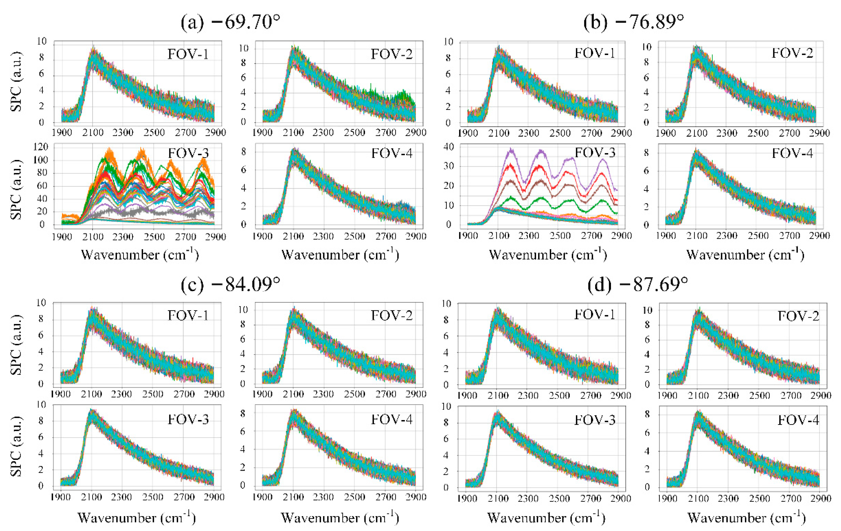
3. SSM Pointing Angle Adjustment for Stray Light Evasion

Based on the solar stray light analysis and propagating simulation, on 13 December 2019, the SSM pointing angle for a cold view was adjusted step by step for stray light evasion (see Figure 8). The candidate angles were tested from −62.5° to −95° (see Table 1) with the DS SWIR raw spectra monitored at the same time. Figure 9 shows four cases of SWIR DS spectra from the four FOVs, corresponding to the angles of −69.70°, −76.89°, −84.09°, and −87.69°. It was found that within the magnitude fluctuation caused by the temperature variation of the instrument’s internal components, the DS spectra could be maintained stable and consistent all over the orbits when the pointing angle is beyond −84.09°. Eventually, the cold space view angle is adjusted from −77.4° to −87°.
After the pointing angle adjustment, the HIRAS-CrIS SNOx data on 14 December 2019 were collected. The HIRAS-CrIS BT differences in the two channels of 1500 cm−1 and 2450 cm−1 are shown in Figure 10 subplots (a) and (b), respectively. Comparing the figure with Figure 6, one can see that although the SNOx data set size in Figure 10 is smaller due to the orbit difference between the two satellites, it is clear that the stray light contamination disappears in both subplots. For the 1500 cm−1 channel, the mean BT difference in the previous contamination zone is μc = −0.412 K with a standard deviation of σc = 0.633 K, and globally is μg = −0.642 K with σg = 0.683 K. For the 2450 cm−1 channel, the mean BT difference in the contamination latitudes is μc = −0.157 K with σc = 2.85 K, and globally is μg = −0.728 K with σg = 3.57 K. Compared to the statistical numbers shown in Figure 6, the statistics of the BT biases relative to CrIS observations are largely improved. In addition to the SNOx data set, the HIRAS imaginary radiance data on the same day are also collected and the data set at 1500 cm−1 is shown in Figure 11. The grey strip shown in Figure 7 disappears in Figure 11 after the DS view angle adjustment.

4. Correction Algorithm for Historic Contaminated Data and Accuracy Assessment to Re-Calibrated Radiance

4.1. Time Series of DS Spectral Integrated Energy

Despite DS spectra contamination by the solar stray light being avoided after the cold view angle adjusting, there are several months of data with contaminated cases that need to be reprocessed. In order to identify the erroneous data, we first define a variable named spectral Integrated Energy (IE) for monitoring the DS spectral orbital variations. The IE value is calculated by cumulating all magnitudes of the DS raw spectrum over the wavenumber abscissa. It represents the integral energy of the DS spectrum, which is mainly contributed by the internal radiation component in normal conditions. Figure 12 shows three hours of the IE time series for all FOVs and all bands spanning two flight orbits. In the LWIR and MWIR subplots, the FOV-3 IE curves present periodically IE wells, while in the SWIR subplot, bursts occur on all IE curves with the strongest bursts on the FOV-3 curve. The abnormal changes of the IE values are caused by the solar light intrusion.

4.2. Method for Correcting DS Contaminated Spectra Based on IE Breakpoint Detection

As shown in Figure 12, in normal conditions, the DS IE time series vary slowly and smoothly with time, and the abnormal changes of the IE values indicate the effect of the solar contamination. With an appropriate method, the erroneous data may be identified and then replaced by the normal data near the contamination zone. The key to the method is to determine the anomalous scan lines exactly. It has been tested that a fixed IE threshold does not work appropriately since the IE values still vary under the normal condition as shown in Figure 12.
We developed an algorithm for detecting the erroneous data, or breakpoints, in the IE time series. It derives the data rejection threshold for each IE data segment based on histogram statistics of the data segment in the SWIR band. To reduce the IE series noise level, before separating the data into segments, the IE time series are smoothed with a 5-point moving average filter. A data segment contains 90 consecutive DS IE data points and is defined as a breakpoint detection window (Det-Win). It spans three calibration averaging windows (Avg-Win), each of which contains 30 scan lines as discussed earlier. To compute the histogram of the SWIR data segment, the data are partitioned into equally spaced histogram bins. The bin width should be appropriate to include enough data for statistics, and, in the meantime, at least one bin contains most of the normal data. Therefore, at least one of the three Avg-Wins in the Det-Win should be free of contamination. Based on this fact, the SWIR IE value range and number of the bins are computed using the equations below,
A v g I E = min { [ 1 30 i = 1 30 I E ( i ) , 1 30 j = 31 60 I E ( j ) , 1 30 k = 61 90 I E ( k ) ] } b i n N u m = ceil { max [ I E ( h ) , h = 1 90 ] min [ I E ( h ) , h = 1 90 ] A v g I E }
where min{…} and max{…} return the minimum and maximum elements of an array respectively, and ceil{…} rounds a number to the nearest integer greater than or equal to it. In Equation (3), the average IE in each of the three Avg-Wins is calculated, and the Avg-Win with the minimum value (AvgIE) contains all normal data. Then taking the AvgIE value as the bin width, the 90 IEs are partitioned into an integral number of value bins. The first bin will contain most of the IEs. The next step is to calculate the mean of the smoothed IEs falling into the bin with the maximum count value (i.e., the first bin) as a baseline of the whole Det-Win and the standard deviation of the raw (unsmoothed) IE data corresponding to these smoothed IE data. The standard deviation is used to form a data rejecting threshold of the IE values relative to the baseline mean value. If the absolute difference between the unsmoothed IE and the baseline mean value is larger than the threshold, the IE is marked as a breakpoint and its corresponding DS spectrum is identified as a contaminated spectrum. In practice, three standard deviations (3-sigma) are adopted as the threshold since about 99.7% of the normal values around the baseline are within the threshold interval, assuming a Gaussian-like distribution of the IEs in the maximum count bin. The last step is to replace the contaminated data with the nearest normal ones. This process of breakpoints detection and DS spectra substitution is repeated, moving along with the calibration Avg-Wins until all contaminated spectra are refreshed.
Figure 13 gives an example of the SWIR DS data correction process. Subplot (a) shows the raw and smoothed IE short-time series in a Det-Win, which contains about 30 anomalous values. In subplot (b), a histogram with 22 bins is calculated according to Equation (3). The first bin contains normal 58 smoothed IEs, shown as red dots in subplot (c). In subplot (c), the two red horizontal lines are the IE 3-sigma thresholds. The IEs outside the thresholds are marked as breakpoints and replaced with the blue dots which are the nearest normal ones on both sides of the contaminated series. Subplot (d) presents the refreshed DS spectra with reasonable continuity in comparison with that in subplot (a) of Figure 5.
The method discussed above is also applied to the data that contain many Det-Wins with no breakpoints. For the widespread normal Det-Wins, the correction method should not be harmful to the normal data. In these normal cases, the histogram only has one bin calculated using Equation (3), since the normal IE fluctuation span is generally smaller than the AvgIE value and the nearest greater integer number is 1. Thus, very few breakpoints would exist under the 3-sigma rule. Figure 14 gives a normal case for data selected on 2 June 2018.
For the LWIR and MWIR bands, the same indexes of the anomalous and nearest normal scan lines detected in the SWIR band are synchronously applied to correct the anomalous data with the nearest normal data in these two bands, so the DS spectra replacement is also performed synchronously. Figure 15 shows the same IE time series as Figure 12 except that the correction is performed to the IE data in Figure 15. It can be seen that the anomalous IEs in the contamination zone are correctly identified and replaced with the nearest normal ones. The uncertainty of the replacement is within the normal orbital variation of the DS spectra in the 5-min period of the Avg-Win.

4.3. Historic Data Re-Calibration and Correction Algorithm Validation

Following the DS spectra refreshing, a set of historic data is collected for the re-calibration test. In the test, the improvement of the ES radiance spectra due to the contaminated DS spectra correction are assessed by comparing the HIRAS-CrIS SNOx statistics before and after the correction. In addition, the improvement is also assessed by checking the imaginary radiance data and the BT differences among FOVs.
For the HIRAS-CrIS SNOx comparison, the HIRAS data set used for Figure 6 is recalibrated and the SNOx BT differences are shown in Figure 16. One can see that the deep blue stripe at 1500 cm−1 in Figure 6a disappears in Figure 16a after the correction of the contaminated data. The mean and standard deviation of the BT differences are improved on a global scale from μg = −1.29 K with σg = 2.05 K to μg = −0.442 K with σg = 0.798 K, and in the contamination zone from μc = −4.73 K with σc = 2.71 K to μc = −0.101 K with σc = 0.623 K. Furthermore, the renewed imaginary radiances data in the contamination zone shown in Figure 17 are also ameliorated greatly in comparison with those in Figure 7.
For the SWIR channel of 2450 cm−1, the HIRAS-CrIS SNOx BT differences after the correction are shown in Figure 16b. As discussed before, since the solar stray lights dominate the DS SWIR spectra, the SNOx biases in the contamination zone are positive. It can be seen that the deep red stripe in Figure 6b disappears in Figure 16b. The mean and standard deviation on the global scale are improved from μg = 1.85 K and σg = 7.49 K to μg = −0.12 K with σg = 3.41 K, and in the contamination zone from μc = 12.2 K and σc = 12.1 K to μc = −0.155 K and σc = 3.01 K.
For all channels and bands, the mean and standard deviation result of the HIRAS-CrIS SNOx BT differences on 7 December 2019 is shown in Figure 18. The SNOx data set for Figure 18 only contains data in the contamination zone and has a total sample number of 11,672. In Figure 18, the results before and after the correction are presented in the left and right columns, respectively, with the top panels showing the spectral range, middle panels the mean biases, and bottom panels the standard deviation. Note that the scale difference of the y-axes between the left and right panels for the bias and standard deviation plots. It can be seen that the solar stray lights significantly contaminate the MWIR and SWIR bands. Without the correction, the radiance biases are negative in the MWIR band with magnitudes of up to 8 K, and positive for the SWIR band with magnitudes of up to 25 K. The magnitudes of the biases in many channels exceed 5 K in the MWIR band and 20 K in the SWIR band. After the correction, the BT biases are less than 0.5 K for most of the channels, except in the MWIR CH4 absorption and SWIR CO2 absorption regions. The standard deviations are also improved significantly from up to 10 K to no more than 2 K in the MWIR band, and 30 K to 8 K in the SWIR band. For the LWIR band, the magnitude of the cold view contamination seems too small to significantly impact the ES radiance calibration. There are little changes in biases and standard deviations before and after the correction for the LWIR band. After the correction, the biases and standard deviations of the HIRAS-CrIS comparison are consistent with those routinely computed with the SNO technique in the HIRAS data monitoring system [6].
In addition to the SNO technique, a so-called FOV-to-FOV consistency check is also applied to assess the quality of the calibrated radiances. In this situation, the reference FOVs are those free of solar stray light contamination. As discussed earlier, the solar stray lights do not contaminate the FOV-1 and FOV-4 data in the LWIR and MWIR bands, but still have a detectable impact on the two FOVs in the SWIR band (see Figure 12). Therefore, in the consistency checking, FOV-1 and FOV-4 are used as reference FOVs for the LWIR and MWIR bands only. The data sample selection criteria are that (1) data only in the contamination zone are considered, and (2) the FOVs in the same FOR are homogenous across the FOVs. In order to satisfy condition (2), the scan angles of the FOVs are limited to within ±10° (including 5 FORs) with respect to the nadir direction and over an oceanic region. A data set with a sample size of 2019 is obtained after applying the above criteria to the observations on 7 and 8 of December 2019. In Figure 19, subplots (a1) and (a2) show the BT differences of FOV-3 with those measured in the FOV-1, and subplots (b1) and (b2) show the BT differences of FOV-3 with FOV-4. In the figure, the left and right columns are the results before and after the corrections of the FOV-3 DS spectra, respectively. It can be seen that the statistical results between the uses of the two references, FOV-1 and FOV-4, are similar. Furthermore, compared to the LWIR and MWIR results shown in Figure 18, they are also similar to those from the SNOx comparison. The FOV-to-FOV comparisons provide additional results in demonstrating the significant improvement of the recalibrated spectra.
The residual error of the correction process is the difference between the radiance data sets: one calibrated with the correction of the contaminated DS spectra and the other calibrated with the same raw spectra except the DS spectra are not contaminated. The small residual error may come from the following two factors. One is the natural fluctuation of the DS spectra during the 5-min observations in the contamination zone, which is difficult to be addressed with the substitution algorithm. The other is that a few DS spectra lightly affected by the solar stray lights may be identified as normal data. The effect of the misidentification should be very small since the DS spectra used in the calibration equation is an average of 30 consecutive samples.

5. Conclusions

Before 13 December 2019, the FY-3D/HIRAS cold space calibration view was susceptible to solar stray light intrusion when the satellite flew towards the end of a descending orbit. This problem could occur in winter and spring when the solar zenith angle is in the range from 100° to 120°. Based on the stray light analysis and calibration assessment, the cold space viewing angle was adjusted from −77.4° to −87° on 13 December 2019, and as a result, the solar light contamination issue was resolved.
As for the historic data, the contaminated DS spectra introduce a negative calibration bias in the MWIR band and a large positive bias in the SWIR band. A DS spectrum substitution method is developed to correct the data damaged by the solar stray light intrusion. The correct method uses histogram statistics of the DS spectral IE time series to detect the anomalous data points and then replace their corresponding DS spectra with the nearest normal ones. In the validation process, historic data are recalibrated after the DS spectra are processed by the correction method. The recalibrated radiance data are evaluated by comparing them with those measured by SNPP/CrIS using the SNOx technique and by checking the HIRAS imaginary radiance data and FOV-to-FOV differences. Both the HIRAS-CrIS comparison and the HIRAS FOV-to-FOV comparison show that, without the correction, the biases of the FOV-3 radiance data can be larger than −5 K in the MWIR band and 20 K in the SWIR bands, and after the correction, the radiance biases are back to the values under the normal conditions: less than 0.5 K in the MWIR band and SWIR CO and window regions, and about 1.5 K in the SWIR CO2 absorption channels.

Author Contributions

Conceptualization, L.L. and C.Q.; methodology, L.L., C.W., M.G. and C.S.; software, L.L., C.W. and M.Y.; validation, L.L., M.Y. and C.Q.; formal analysis, L.L.; investigation, X.H.; resources, X.H. and P.Z.; data curation, X.H.; writing—original draft preparation, L.L. and C.W.; writing—review and editing, L.L., C.W., C.Q. and X.H.; visualization, L.L. and M.Y.; supervision, X.H. and P.Z.; project administration, X.H.; funding acquisition, C.Q. All authors have read and agreed to the published version of the manuscript.

Funding

This research was funded by the National Satellite Meteorological Center (NSMC) of China Meteorological Administration (CMA) under the program of Calibration Technology Development and Level-1 Data Production for the Hyperspectral Imaging and Sounding Instruments onboard FY-3E and FY-4B Satellites, FY-APP-2021.0507.

Acknowledgments

We are grateful to Fabien Carminati and Xianjun Xiao for their useful discussions that helped us improve this study.

Conflicts of Interest

The authors declare no conflict of interest. The funders had no role in the design of the study; in the collection, analyses, or interpretation of data; in the writing of the manuscript, or in the decision to publish the results.

References

  1. Menzel, W.P.; Schmit, T.J.; Zhang, P.; Li, J. Satellite-based Atmospheric Infrared Sounder Development and Application. Bull. Am. Meteorol. Soc. 2018, 99, 583–603. [Google Scholar] [CrossRef]
  2. English, S.J.; Renshaw, R.J.; Dibben, P.C.; Smith, A.J.; Rayer, P.J.; Poulsen, C.; Saunders, F.W.; Eyre, J.R. A comparison of the impact of TOVS and ATOVS satellite sounding data on the accuracy of numerical weather forecasts. Q. J. R. Meteorol. Soc. 2000, 126, 2911–2931. [Google Scholar] [CrossRef]
  3. Hilton, F.; Atkinson, N.C.; English, S.J.; Eyre, J.R. Assimilation of IASI at the Met Office and assessment of its impact through observing system experiments. Q. J. R. Meteorol. Soc. 2009, 135, 495–505. [Google Scholar] [CrossRef]
  4. Smith, A.; Atkinson, N.; Bell, W.; Doherty, A. An initial assessment of observations from the Suomi-NPP satellite: Data from the Cross-track Infrared Sounder (CrIS). Atmos. Sci. Lett. 2015, 16, 260–266. [Google Scholar] [CrossRef]
  5. Hilton, F.; Armante, R.; August, T.; Barnet, C.; Bouchard, A.; Camy-Peyret, C.; Capelle, V.; Clarisse, L.; Clerbaux, C.; Coheur, P.F.; et al. Hyperspectral Earth observation from IASI: Five years of accomplishments. Bull. Am. Meteorol. Soc. 2012, 93, 347–370. [Google Scholar] [CrossRef]
  6. Qi, C.; Wu, C.; Hu, X.; Xu, H.; Lee, L.; Zhou, F.; Gu, M.; Yang, T.; Shao, C.; Yang, Z.; et al. High Spectral Infrared Atmospheric Sounder (HIRAS): System Overview and On-Orbit Performance Assessment. IEEE Trans. Geosci. Remote Sens. 2020, 58, 4335–4352. [Google Scholar] [CrossRef]
  7. Wu, C.; Qi, C.; Hu, X.; Gu, M.; Yang, T.; Xu, H.; Lee, L.; Yang, Z.; Zhang, P. FY-3D HIRAS Radiometric Calibration and Accuracy Assessment. IEEE Trans. Geosci. Remote Sens. 2020, 58, 3965–3976. [Google Scholar] [CrossRef]
  8. Revercomb, H.E.; Buijs, H.; Howell, H.B.; La Porte, D.D.; Smith, W.L.; Sromovsky, L. Radiometric calibration of IR Fourier transform spectrometers: Solution to a problem with the high-resolution interferometer sounder. Appl. Opt. 1988, 27, 3210–3218. [Google Scholar] [CrossRef] [PubMed]
  9. Han, Y.; Chen, Y. Calibration algorithm for cross-track infrared sounder full spectral resolution measurements. IEEE Trans. Geosci. Remote Sens. 2018, 56, 1008–1016. [Google Scholar] [CrossRef]
  10. Carminati, F.; Xiao, X.; Lu, Q.; Atkinson, N.; Hocking, J. Assessment of the Hyperspectral Infrared Atmospheric Sounder (HIRAS). Remote Sens. 2019, 11, 2950. [Google Scholar] [CrossRef] [Green Version]
  11. Schreiber, J.; Blumenstock, T.; Fischer, H. Effects of the self-emission of an IR Fourier-transform spectrometer on measured absorption spectra. Appl. Opt. 1996, 35, 6203–6209. [Google Scholar] [CrossRef] [PubMed]
  12. Configuration Management Office, GSFC JPSS. Joint Polar Satellite System (JPSS) Cross Track Infrared Sounder (CrIS) Sensor Data Records (SDR) Algorithm Theoretical Basis Document (ATBD) (Revision C); Document Code 474: 474-00032; Goddard Space Flight Center: Greenbelt, MD, USA, 2014; pp. 33–34. Available online: http://docserver.gesdisc.eosdis.nasa.gov/public/project/JPSS-1/JPSS.CrIS.Sensor.Data.Record.ATBD.RevC.Code474_474-00032.pdf (accessed on 26 September 2021).
  13. Cao, C.; Weinreb, M.; Xu, H. Predicting Simultaneous Nadir Overpasses among Polar-Orbiting Meteorological Satellites for the Intersatellite Calibration of Radiometers. J. Atmos. Ocean. Technol. 2004, 21, 537–542. [Google Scholar] [CrossRef]
  14. Wang, L.; Han, Y.; Jin, X.; Chen, Y.; Tremblay, D. Radiometric consistency assessment of hyperspectral infrared sounders. Atmos. Meas. Tech. 2015, 8, 4831–4844. [Google Scholar] [CrossRef] [Green Version]
  15. Cao, C.; Uprety, S.; Blonski, S. Establishing radiometric consistency among VIIRS, MODIS, and AVHRR using SNO and SNOx methods. In Proceedings of the 2012 IEEE International Geoscience and Remote Sensing Symposium, Munich, Germany, 22 July 2012. [Google Scholar] [CrossRef]
  16. Han, Y.; Revercomb, H.; Cromp, M.; Gu, D.; Johnson, D.; Mooney, D.; Scott, D.; Strow, L.; Bingham, G.; Brog, L.; et al. Suomi NPP CrIS measurements, sensor data record algorithm, calibration and validation activities, and record data quality. J. Geophys. Res. Atmos. 2013, 118, 734–748. [Google Scholar] [CrossRef]
  17. Zavyalov, V.; Esplin, M.; Scott, D.; Esplin, B.; Bingham, G.; Hoffman, E.; Lietzke, C.; Predina, J.; Frain, R.; Suwinski, L.; et al. Noise performance of the CrIS instrument. J. Geophys. Res. Atmos. 2013, 118, 13108–13120. [Google Scholar] [CrossRef] [Green Version]
Figure 1. The global distribution of DS raw spectra at 2303 cm−1 along the flight track on 1 February 2019. The spectral anomalies are indicated by the large increase of the spectral magnitude in the descending orbit between 30° S and 60° S.
Remotesensing 13 03869 g001
Figure 2. Same to Figure 1, except for the DS raw spectra at 778.125 cm−1.
Remotesensing 13 03869 g002
Figure 3. Same to Figure 1, except for the DS raw spectra at 1500 cm−1.
Remotesensing 13 03869 g003
Figure 4. The DS SW raw spectra measured in the abnormal zone on the first day of each month from May 2018 to April 2019. Although in the subplot for data on 1 December 2018, there have no surged magnitudes, it has found the anomalous spectra occurred in the last several days of that month.
Remotesensing 13 03869 g004
Figure 5. The time series of FOV-3 DS spectra within a ten-minute period illustrate the distortion of the spectra in the three bands. In the SWIR spectra (a), there are spectral bursts at some scan lines, while in the LWIR (b) and the MWIR (c) spectra, the magnitudes at corresponding lines only decline to some degree.
Remotesensing 13 03869 g005
Figure 6. SNOx BT differences (biases) between the HIRAS FOV-3 and SNPP/CrIS observations at the MWIR 1500 cm−1 channel (a) and the SWIR 2450 cm−1 channel (b) on 7 December 2019 (BT difference = BTHIRASBTCrIS). μ and σ represent the mean and standard deviation of the BT differences, respectively: μg and σg on the global data set, and μc and σc on the data set limited in the contamination zone between 30° S to 60° S.
Remotesensing 13 03869 g006
Figure 7. The global distribution of FY-3D/HIRAS (all FOVs) imaginary radiances at 1500 cm−1 on 7 December 2019.
Remotesensing 13 03869 g007
Figure 8. HIRAS scanning mode diagram.
Remotesensing 13 03869 g008
Figure 9. DS SWIR spectra at different SSM DS pointing angles during the stray light evasion test on 13 December 2019.
Remotesensing 13 03869 g009
Figure 10. Same to Figure 6 except that the SNOx data set is on 14 December 2019 after the DS pointing angle adjustment.
Remotesensing 13 03869 g010
Figure 11. Same to Figure 7 except that the imaginary data set is on 14 December 2019 after the DS pointing angle adjustment.
Remotesensing 13 03869 g011
Figure 12. Three-hour IE time series spanning two flight orbits. Upper panel—LWIR, middle panel—MWIR, and bottom panel—SWIR. Different FOVs are coded in different colors and the smooth black curves are the results of a 5-point moving average filter.
Remotesensing 13 03869 g012
Figure 13. An example of the anomalous DS SWIR correction process and result. (a): the raw IE time-series in a Det-Win (green line), and the smoothed series calculated by a 5-point moving average filter (black line). (b): the smoothed IE histogram with 22 value bins defined by Equation (3). (c): red dots are IEs in the bin with the maximum number count, the two red horizontal lines are the 3-sigma of the standard deviation thresholds (see text for details), and the blue dots are the replacements to the data points beyond the thresholds with the nearest data points within the threshold. (d): the refreshed DS spectral series; and the green, purple, red, sky-blue, and blue line are spectra with scan index 1, 18, 29, 45, and 60, which are as same as those in Figure 5 (a).
Remotesensing 13 03869 g013
Figure 14. Same to Figure 13 except for a normal case. (a): the raw IE time-series in a Det-Win (green line), and the smoothed series calculated by a 5-point moving average filter (black line). (b): the smoothed IE histogram with only one value bin calculated by Equation (3). (c): red dots are IEs in the bin with the maximum number count, the two red horizontal lines are the 3-sigma of the standard deviation thresholds, and the blue dots are same to the green raw IEs, since they are originally the normal ones within the threshold. (d): the originally normal DS spectral series; and the green, purple, red, sky-blue, and blue line are spectra with scan index 1, 18, 29, 45, and 60, which are as same as those in Figure 5 (a).
Remotesensing 13 03869 g014
Figure 15. Same to Figure 12 except that the data are reprocessed with the correction method.
Remotesensing 13 03869 g015
Figure 16. Same to Figure 6 except the HIRAS radiance data are recalibrated after the DS spectra are processed with correction methods.
Remotesensing 13 03869 g016
Figure 17. Same to Figure 7 except the HIRAS radiance data are recalibrated after the DS spectra are processed with correction methods.
Remotesensing 13 03869 g017
Figure 18. HIRAS FOV-3 spectral distributions (top) of the HIRAS-CrIS SNOx data set on 7 December 2019 in the contamination zone before (left) and after (right) the correction, and the means (middle) and standard deviations (bottom) of the SNOx BT differences. Note that the y-axes scales are different between the left and right panels because the bias and standard deviation before correction are significantly larger than that of correction.
Remotesensing 13 03869 g018
Figure 19. HIRAS LWIR and MWIR BT differences between FOV-3 and normal FOVs in contamination zone before (left) and after (right) correction, (a1,a2) present the comparison of FOV-3 with FOV-1, (b1,b2) of FOV-3 with FOV-4.
Remotesensing 13 03869 g019
Table 1. Pointing angles tested for stray light evasion.
Pointing AngleSpectral Anomalies in FOV-3Spectral Anomalies in FOV-2
−62.50°yesyes
−66.10°yesno
−69.70°yesno
−73.29°yesyes
−76.89°yesno
−80.48°noyes
−84.09°nono
−87.69°nono
−91.30°nono
−94.93°nono
Publisher’s Note: MDPI stays neutral with regard to jurisdictional claims in published maps and institutional affiliations.

